Computing Architectures
Mitigating CFL Bottlenecks for Large-Scale Wave Propagation
Doctoral Dissertation submitted to the
Faculty of Informatics of the Università della Svizzera Italiana in partial fulfillment of the requirements for the degree of
Doctor of Philosophy
presented by
Max Rietmann
under the supervision of
Olaf Schenk
Michael Bader Technische Universität München, Munich, Germany Andreas Fichtner ETH Zürich, Zurich, Switzerland
Marcus Grote Universität Basel, Basel, Switzerland
Rolf Krause Università della Svizzera italiana, Lugano, Switzerland Igor Pivkin Università della Svizzera italiana, Lugano, Switzerland Olaf Schenk Università della Svizzera italiana, Lugano, Switzerland
Dissertation accepted on 12 May 2015
Research Advisor PhD Program Director
Olaf Schenk Igor Pivkin
presented in this thesis is that of the author alone; the work has not been sub-mitted previously, in whole or in part, to qualify for any other academic award; and the content of the thesis is the result of work which has been carried out since the official commencement date of the approved research program.
Max Rietmann
Lugano, 12 May 2015
not fool yourself and you are the easiest person to fool.
Richard P. Feynman
Modeling problems that require the simulation of hyperbolic PDEs (wave equa-tions) on large heterogeneous domains have potentially many bottlenecks. We attack this problem through two techniques: the massively parallel capabilities of graphics processors (GPUs) and local time stepping (LTS) to mitigate any CFL bottlenecks on a multiscale mesh. Many modern supercomputing centers are installing GPUs due to their high performance, and extending existing seismic wave-propagation software to use GPUs is vitally important to give application scientists the highest possible performance. In addition to this architectural opti-mization, LTS schemes avoid performance losses in meshes with localized areas of refinement. Coupled with the GPU performance optimizations, the derivation and implementation of an Newmark LTS scheme enables next-generation per-formance for real-world applications. Included in this implementation is work addressing the load-balancing problem inherent to multi-level LTS schemes, en-abling scalability to hundreds and thousands of CPUs and GPUs. These GPU, LTS, and scaling optimizations accelerate the performance of existing applica-tions by a factor of 30 or more, and enable future modeling scenarios previously made unfeasible by the cost of standard explicit time-stepping schemes.
The content of this thesis benefited greatly from the input and help of a number of people, including the coauthors of our published, accepted, and in-progress works. In particular, Piero Basini and Peter Messmer provided meshing and opti-mization help for our original GPU paper that motivated the GPU chapter. Daniel Peter’s knowledge of SPECFEM3D was invaluable when implementing LTS. Bora Uçar’s suggestion to use hypergraphs improved the work on load balancing our LTS implementation. The LTS work itself was greatly influenced by discussions and input from Marcus Grote. I thank my advisor Olaf Schenk for his academic and financial support, the University of Basel, the ETH Zurich, CSCS, and the USI Lugano for their support in all manners of my PhD. Finally, I thank my PhD committee, who agreed to take the time to provide useful feedback and ques-tions regarding this thesis and the work leading up to it.
Contents ix
1 Introduction 1
1.1 Wave-Propagation Application: Seismology . . . 2
1.1.1 Earthquake simulation example . . . 3
1.1.2 Increased performance using graphics processors . . . 7
1.1.3 Mitigating time stepping bottlenecks . . . 7
1.2 Summary and Outline . . . 9
2 Wave Propagation on Emerging Architectures 11 2.1 GPU Background . . . 13
2.1.1 GPU vs. CPU architecture . . . 14
2.2 Roofline Model . . . 15
2.2.1 Matrix operation benchmarks . . . 17
2.2.2 CUDA programming model . . . 18
2.2.3 Related work . . . 19
2.3 SPECFEM3D GPU . . . 21
2.3.1 The spectral element method for GPUs . . . 22
2.3.2 SEM computational structure . . . 27
2.4 GPU performance optimizations . . . 29
2.5 Performance Evaluation . . . 38
2.5.1 Benchmarking GPU versus CPU simulations . . . 39
2.5.2 Weak scaling . . . 40
2.5.3 Strong scaling . . . 41
2.5.4 Large application test . . . 43
2.6 Roofline Model for SPECFEM3D . . . 45
2.6.1 Emerging architectures outlook . . . 47
2.7 Adjoint Tomography . . . 48
2.7.1 Adjoint methods overview . . . 48 ix
2.7.2 Adjoint costs . . . 50
2.7.3 I/O optimizations . . . 51
2.7.4 Adjoint performance benchmarks . . . 54
2.8 Conclusion . . . 55
3 Newmark Local Time Stepping 59 3.1 Introduction . . . 60
3.2 Newmark Time Stepping for Wave Propagation . . . 61
3.2.1 Newmark time stepping . . . 62
3.2.2 Comparison with leapfrog . . . 65
3.2.3 Conservation of energy . . . 66
3.2.4 Fine and coarse element regions . . . 66
3.2.5 LTS-Newmark . . . 67
3.3 Single-Step Method . . . 69
3.3.1 LTS as modification to matrix B . . . . 72
3.3.2 Equivalence to LTS-leapfrog . . . 73
3.4 Absorbing Boundaries . . . 73
3.4.1 Multiple refinement levels . . . 75
3.4.2 Single step equivalent for multiple levels . . . 78
3.5 LTS-Newmark for Continuous Elements . . . 80
3.5.1 Implementation detail . . . 83
3.6 Numerical Experiments . . . 84
3.6.1 Numerical convergence . . . 84
3.6.2 Stability and CFL invariance . . . 86
3.7 Implementation in Three Dimensions . . . 90
3.7.1 Implementation in SPECFEM3D . . . 90
3.7.2 Experiments in three dimensions . . . 91
3.7.3 LTS evaluation and validation . . . 91
3.7.4 LTS scaling . . . 92
3.8 Conclusions . . . 94
4 Load-Balanced Local Time Stepping at Scale 95 4.1 Introduction . . . 96
4.2 The Partitioning Problem . . . 96
4.2.1 LTS-Partition models: graphs and hypergraphs . . . 99
4.2.2 Partitioning algorithms for LTS . . . 103
4.3 Performance Experiments . . . 104
4.3.1 Application mesh benchmarks . . . 104
4.3.3 CPU and GPU performance results . . . 108
4.3.4 Cache performance . . . 111
4.3.5 Large example . . . 112
4.3.6 Application example: Tohoku . . . 113
4.3.7 Additional partitioning options . . . 115
4.4 Conclusion . . . 116
5 Conclusions and Outlook 119 5.1 Summary . . . 120
5.2 Revisited: Application Example . . . 122
5.3 Final Discussion . . . 125
Introduction
This thesis is presented as a work of computational science; a multidisci-plinary effort bringing together computing and algorithmic advancements to greatly accelerate large-scale scientific applications. Although the work in this thesis is generally applicable, we are particularly focused on the efficient simu-lation of wave propagation at large computational scales — both in the problem size considered and the resources used. This is achieved in three parts:
1. high-performance implementations for newly developed graphics-processing computing architectures;
2. mitigating time-stepping bottlenecks via local time stepping (LTS); 3. load-balanced LTS for many-node supercomputing clusters.
Each of these points represents a separate contribution, each independently and dramatically increasing the performance of our newly developed additions to an existing software package. Critically, each component’s performance can be combined to drastically improve performance over the original implementation. The techniques developed and derived in this thesis can be generally ap-plied; we have, however, specifically targeted computational seismology, which uses numerical computing to study seismic phenomena such as earthquakes. In particular, seismology is focused on the propagation and interaction of an earth-quake’s waves with the Earth’s crust, mantle, and core. Computational seismol-ogy tries to simulate these waves using (quasi-)analytical and purely numerical methods. The large simulation domain (the entire Earth or portions of it) cou-pled with the large number of events simulated means that seismology has been pushing the boundaries of high-performance computing (HPC) for years. This thesis aims to both bring higher performance through the use of new classes of computing devices, but also to enable localized modeling that previously created drastic performance reductions due to time-stepping stability criteria. In order to motivate these enhancements, we detail an application example to highlight the computational costs and bottlenecks this thesis is trying to reduce or eliminate.
1.1
Wave-Propagation Application: Seismology
Like many scientific disciplines, seismology is driven forward by theoretical ad-vances coupled to real data of increasing quality and volume. As seismologists collected more and better seismogram data (displacement, velocity, and accel-eration recordings based on ground motion from earthquakes or other seismic sources), it became possible to characterize the propagation of seismic waves
through the Earth. In order to better understand the propagation of these waves, partial different equations (PDEs) modeling acoustic and elastic domains were developed to describe the propagation of waves through the earth. In order to solve these models, various numerical techniques exist to simulate these waves. From the perspective of a numerical modeler, the Earth can be represented by a surprisingly simple linear PDE-model, with a thin crust, a large elastic mantle, and a (mostly) reflecting core. 3D simulations run on such a model can agree, to an initial estimation, quite well with real recorded seismograms. However, by analyzing the fit between real and simulated data, we can make improvements to this simple earth model that potentially reveal interesting physical properties about the Earth’s internal structure.
1.1.1
Earthquake simulation example
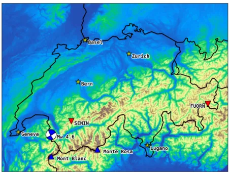
To make this discussion concrete, we present an example to compare real data recorded in Switzerland with a simulation using our seismic wave-propagation research package SPECFEM3D. To be more formally introduced in later chap-ters, SPECFME3D [Peter et al., 2011] is a comprehensive software program to simulate the viscoelastic wave equation on hexahedral finite-element meshes on large-scale supercomputing systems. In other words, we can simulate earth-quakes on a discrete domain to approximate and evaluate our spatial parameters (p- and s-wave velocities, density, etc) and source model (moment tensor, time, and location). With this in mind, we selected a real event and appropriate seis-mogram traces from recording stations to evaluate our ability to replicate the real data, with the setup seen in Fig. 1.1.
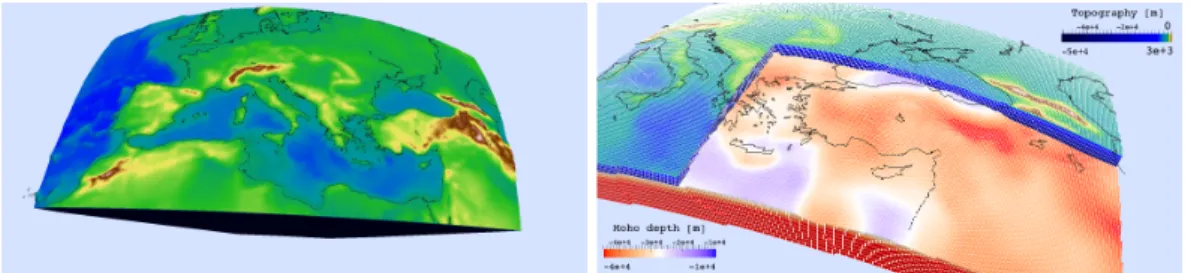
The two stations FUORN (east Switzerland) and SENIN (west Switzerland) recorded a magnitude (Mw) 4.6 earthquake on September 08, 2005 at 11:27:22 AM, located in the Swiss-French Alps at a relatively shallow depth of 10 km. In order to simulate this earthquake in SPECFEM3D, we need a hexahedral mesh that covers the simulation domain with enough resolution to resolve the waves as they propagate from the source to the two receivers. The setup, with 5 km elements and the appropriate topography profile,1 is shown in Fig. 1.2.
This mesh has about 350K elements and 23M degrees of freedom, due to the higher-order nature of the finite-element method used. With a stable time step ∆t = 0.04 s, we simulated 180 s in order to propagate the waves completely through the domain. Thus, we needed 180/∆t = 4500 steps, requiring 40 min of wall-clock time on a modern 8-core Intel CPU.
Figure 1.1. Earthquake simulation setup, with a Mw 4.6 earthquake in the Swiss-French Alps and two recording stations FUORN and SENIN.
For this example, we use a 1D or depth-only velocity profile [Diehl et al., 2009], which does not contain horizontal (x-y) variations. This depth-only ve-locity profile deviates only slightly from the well-known PREM model, which provides a global average profile and forms the basis of most velocity models.
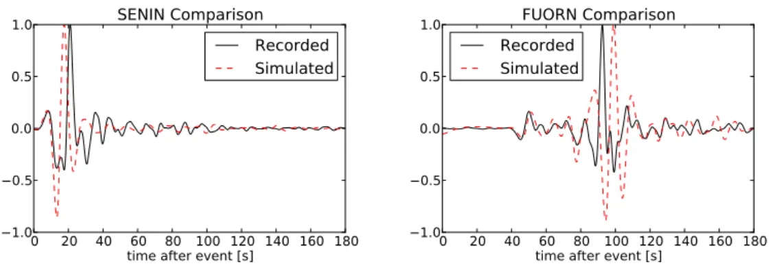
Obtaining real data to compare with our simulation has also become much faster and easier than previously. Using the ObsPy seismology library[Beyreuther et al., 2010] to access the freely available IRIS database, we collected seismo-gram traces for the FUORN and SENIN stations for several minutes directly fol-lowing the earthquake. This includes the respective instrument responses, allow-ing us to match our simulation to real, recorded data. After application of the instrument response, bandpass filtering between 60 and 10 s (1/60 and 1/10 Hz), and normalization we attained the seismogram comparisons for the two stations FUORN and SENIN for the z-component of the velocity seen in Fig. 1.3. For a nonseismologist, the compared graphs may not look especially impres-sive, however, given that we are comparing a relatively simple model to data from a real earthquake recorded at a station in the mountains, the result is fairly promising. The energy that creates seismic waves, such as those seen here, propagates through the Earth along different ray paths. The first arrivals (the first small bump seen) travel through the Earth in an upwards parabolic trajec-tory (due to Snell’s law). The slower surface velocity ensures that the larger
Figure 1.2. Hexahedral mesh domain with topography and our 1D (z-dir) veloc-ity model covering our experimental setup in Switzerland. Mesh elements are approximately 5 km across. Note that p-wave velocity goes from 5800 m/s in the crust to 8700 m/s at a depth of 300 km.
surface-traveling waves arrive later (the stronger oscillations seen after the ini-tial arrival). Thus, we see that the qualitative nature of the seismograms, which includes the arrival time of different wave components, is positive. Considering the FUORN graphs, the initial small bump, 40 s after the event, represents the direct wave, which travels through the medium and arrives at nearly the same time in both simulated and real data. The arrival of the larger peaks appear-ing later that represent surface waves is also very good. On the other hand, the general shape of the seismograms does leave room for improvement. Addi-tionally, if we had raised the frequency cap on the bandpass to a higher cutoff, we would see further disagreement indicating that the smaller-scale variations are important and worth trying to improve for our horizontally homogeneous velocity model.
Although there are several techniques for improving the spatial velocity and density parameters (“the model”), we are particularly interested in a technique called full waveform inversion (FWI), which uses these simulations to construct linearized model updates, which are combined with nonlinear optimization tech-niques to iteratively improve the model by reducing the misfit (error) between real and simulated seismogram traces. A single earthquake event will not pro-vide enough so-called “coverage” to improve the velocity model to a substantial degree. We will need to add significantly more earthquake sources to adequately resolve all of Switzerland. In Fig. 1.4, we map 168 earthquakes from the last 10–
0 20 40 60 80 100 120 140 160 180 time after event [s]
1.0 0.5 0.0 0.5 1.0 SENIN Comparison Recorded Simulated 0 20 40 60 80 100 120 140 160 180 time after event [s]
1.0 0.5 0.0 0.5 1.0 FUORN Comparison Recorded Simulated
Figure 1.3. Comparison between real (recorded) and simulated (with SPECFEM3D) seismograms of z-component velocity for SENIN and FUORN. Filtered between 1/60 and 1/10 Hz and normalized.
15 yr, which could be used to do this for Switzerland. Each incremental model update requires several simulations per earthquake, and the iterative process can require many steps. Facing the cost of these many simulations, we are motivated to improve the performance of our simulation software to reduce the cost and pain associated with waiting for so many simulations.
168 events (2001-01-20 to 2013-12-12) with Mw 3.0 - 5.0
3.0 3.5 4.0 4.5 5.0
Magnitude
1.1.2
Increased performance using graphics processors
At the beginning of this research, NVIDIA’s newest compute-only graphics pro-cessors (GPUs) were just becoming popular enough that supercomputing centers were building small development clusters. It was hoped that these newly devel-oped GPU “accelerators” would drastically improve performance for many fields in science, including computational seismology. Thus we have explored their use and detail the development of a GPU-capable software package for wave-propagation problems in Ch. 2. There we introduce extensions of the code to not only run these earthquake simulations, but also compute model updates to improve the match between real and simulated seismograms via adjoint to-mography techniques, which should dramatically improve upon existing CPU performance.
To give a taste of these improvements, the simulation that required 40 min on a high-end 8-core CPU requires less than 6 min of wall-clock time using a single NVIDIA Tesla K20c GPU. However, this performance comes at a high de-veloper cost to port the existing CPU code to the GPU, which has a dramatically different programming model and set of critical optimizations in order to achieve the 6 min simulation time. We were able to match the wave-propagation com-putational structure to the threading model employed by GPUs, in addition to the cache and memory optimizations necessary to attain even adequate perfor-mance[Rietmann et al., 2012]. These performance improvements are, however, limited by the numerical techniques underlying the implementation. In partic-ular, we are additionally interested in algorithmic advancements that can be coupled with the GPU speedup to yield double digit factors of improved perfor-mance.
1.1.3
Mitigating time stepping bottlenecks
Simply using the GPU improvements from Ch. 2, we can get a factor 5–7x shorter simulation times, drastically decreasing the time needed to update the model, or, conversely, increasing the coverage or detail we can achieve given an already fixed computational budget. However, as noted, the time-step size ∆t factored directly into the cost (via the 180/∆t = 4500 required steps). The finite ele-ment mesh presented in this introduction is relatively homogeneous, despite the topography on the surface. In this Switzerland model, if we are interested in topography with additional detail, modeling of sediment layers, or any physical modeling that requires locally increased resolution, the impact on the time step ∆t can drastically impact the simulation performance due to the CFL stability
criterion for standard explicit time-stepping schemes which specifies that
∆t ≤ CCFLhmin, (1.1)
where hmin is proportional to the radius of the smallest element in the mesh and
CCFL is a constant that depends on the spatial discretization and time-stepping method. For this mesh in Switzerland, we additionally introduce a refinement around the source such that the smallest element is 32 times smaller than the largest, which can be seen in Fig. 1.5. This refinement results in a factor of 32x increase in simulation time due to the smaller time steps required to ensure stability when using a traditional time-stepping scheme. This translates to 2 hours 25 minutes for the GPU (compared to 6 minutes), and more than 16 hours for a single 8-core CPU (compared to 40 minutes). This drastic increase in simulation time is due to a very small fraction of the total elements — only 3% of the elements are 2x or more smaller than the bulk of elements in the mesh. This means that 97% of elements are taking a time step that is 32x smaller than needed.
Figure 1.5. Refinement around source with smallest element hmin = hmax/32.
The first layer of refinement can be seen close to the source location at the surface (left panel), and the zoom/cut (right panel) shows the smallest elements buried at the source location.
From a physical perspective, this simplistic refinement is difficult to motivate directly, but it does present a model for us to mitigate the drastic efficiency problems for a variety of practical applications. For example, in Ch. 4 we present an application where small elements arise when using a fault-rupture source model, which expands the traditional single-element earthquake source along a
fault, which must be honored by the finite element mesh, creating a localized region of small elements. Explicit time-stepping schemes such as the Newmark scheme (used in SPECFEM3D) are forced to take small time steps, which, as seen, dramatically increase simulation times. In Ch. 3 we derive an explicit LTS scheme that can take steps that are matched with the element size. This drastically reduces the amount of required computation, thus reducing the loss in performance due to the CFL stability criteria in (1.1).
Motivated by these applications in seismology, this thesis contributes not only a newly developed LTS-Newmark scheme for general use in wave propagation, but also an implementation on both CPUs and GPUs that can run on large-scale problems, with billions of degrees of freedom, within the well-known software package SPECFEM3D [Rietmann et al., 2014]. This LTS implementation has also been made parallel-ready [Rietmann et al., 2015], the contribution to be detailed in Ch. 4. This means we can run our LTS-Newmark scheme on meshes with millions of elements across hundreds of CPUs and GPUs, while maintain-ing parallel efficiency. As these contributions have been integrated into the SPECFEM3D package, they will be ready for use by real application seismolo-gists, hopefully enabling applications that were previously too expensive due to the pure computational complexity, or due to CFL limitations from small ele-ments.
1.2
Summary and Outline
We begin the thesis in Ch. 2 where we introduce the spectral finite element method, the seismology package SPECFEM3D, graphics processors (GPUs) for computing, and our GPU extensions to SPECFEM3D to take advantage of these emerging HPC devices. We present work that accelerates both earthquake simu-lations and tomography projects to improve the fit between data and simulation, as seen in Fig. 1.3. These improvements provide the first component of perfor-mance for a next-generation simulation package for general use in seismology.
Following the analysis and use of these emerging computing architectures, Ch. 3 develops the Newmark LTS algorithm for use in cases of localized element refinement, where time-stepping stability requirements can drastically reduce the application performance. We present both theoretical and experimental re-sults to demonstrate the scheme’s convergence and stability, but also specific algorithmic developments that are critical to an efficient implementation when using a continuous finite-element method. Using these techniques, the LTS-Newmark algorithm is efficiently implemented for both CPU and GPU
architec-tures in SPECFEM3D, providing 90%+ of single-threaded LTS efficiency.
Although the seismology example shown in this introduction is capable of running on a single GPU, it is critical that we are able to run with many ad-ditional CPUs and GPUs. Chapter 4 introduces the load-balancing problem that (multilevel) LTS creates and our solution that enables the use of more than 8000 CPUs on large problems with more than 1 billion degrees of freedom, a factor 100 larger than the example provided in this introduction.
Each chapter presents an independent advancement to the tools available to application scientists utilizing simulations of large-scale wave propagation. Significantly, these contributions will be generally available in the open-source SPECFEM3D code, bringing cutting edge simulation performance to computa-tional seismologists, with only a runtime parameter setting. In the conclusion (Ch. 5) we will demonstrate the benefit of each chapter on the earthquake ex-ample provided in this introduction, demonstrating how coupled advances in algorithms and architectures deliver the next generation of performance needed by application scientists.
Wave Propagation on Emerging
Architectures
In 2003, Komatitsch et al. [2003] ran a global earthquake simulation with 14.6 billion degrees of freedom on the Japanese Earth Simulator, using 243 of 640 available nodes. At the time, the Earth Simulator was the number one super-computer (from TOP500), and the resulting paper from these experiments won the Supercomputing Gordon Bell prize. This simulation of the full 3D waveform on a global mesh was a great achievement and the SPECFEM3D software set the standard for efficient MPI-based wave propagation codes.
Since the initial development of SPECFEM3D, it has been split into two pack-ages, one for purely global-scale propagation on a fixed, analytically defined mesh (SPECFEM3D GLOBE). The second, and the target for the work in this thesis, is SPECFEM3D Cartesian, which operates on a user-defined hexahedral mesh, which can be generated in a program such as Trelis (née CUBIT1). Both
are well optimized to simulate the forward model very efficiently on CPUs and are now more limited by physical resolution limitations than by total cluster power or memory. In other words, increasing resolution of the underlying earth model (density, velocity, etc.) is an open research project and defines the current challenge in computational seismology.
As discussed in the introduction, improving the fit between real and synthetic (simulated) seismogram traces is an important application domain in seismol-ogy. This process of imaging the Earth using data from earthquakes and other sources, called tomography, is an inverse procedure that tries to match simu-lated (synthetic) data to real earthquake seismogram recordings. Following the adjoint tomography procedure [Tromp et al., 2004; Peter et al., 2007], many groups are able to utilize existing forward codes, make relatively small changes, and run the many required simulations to calculate a gradient that describes how to iteratively update the earth’s velocity model. Using gradient-only nonlin-ear optimization techniques such as nonlinnonlin-ear conjugate gradient, they are able to update the 3-D seismic velocities, progressively reducing the misfit between the simulations and their real seismogram counterparts measured from actual events.
To do adjoint tomography using the SPECFEM3D package, a database of earthquakes is assembled, corresponding to seismograms recorded at stations within the region of interest. For each earthquake in the database, a forward sim-ulation is compared with actual seismogram data to produce the adjoint source at each recording station. For the second step, both the forward and adjoint fields are simulated, which are compared in order to produce the Fréchet
deriva-1Trelis (originally CUBIT) is a commercially available software package that specializes in mesh generation using hexahedral elements and is currently available through CSimSoft (http://www.csimsoft.com).
tives, or gradient used in the optimization scheme. Each earthquake-source gra-dient is summed to provide the best spatial coverage possible, which is typically given as input to a nonlinear optimization technique such as conjugate gradient or BFGS [Wright and Nocedal, 1999] in order to update the model. Given an appropriate step length, the model update will reduce the misfit between our real data and the simulation. This iterative process continues until the stopping criterion is reached, which can defined by a sufficiently small change in misfit.
Previous regional and global tomographic experiments have shown that this method can converge after 10–30 iterations [Fichtner et al., 2009; Tape et al., 2009; Zhu et al., 2012]. We can thus estimate that the final model will require approximately
3× (number of earthquakes) × (20 steps)
equivalent forward simulations. For a database of 150 earthquakes, we will have 9000 simulations to perform. Depending on the scale of meshes in question, a full inversion using this adjoint tomography procedure requires at least 2 million CPU hours for 150 earthquakes on a smaller regional mesh, and > 700 million CPU hours using a large database of high quality earthquake data of the last ten years on the global scale. Beyond the purely computational challenges associ-ated with these imaging methods, they are inherently ill-posed inverse problems, making them sensitive to details of the methods themselves. It is very common to try and compare several combinations of data filters, preconditioners, update schemes, and regularization terms when updating the model, requiring further sets of simulations, compounding an already difficult problem.
Many levels in the algorithm and software stack of this inverse problem are active areas of research. In this chapter we specifically present the accelera-tion of the forward and adjoint simulaaccelera-tions using graphics processors (GPUs) to increase SPECFEM3D’s performance, thus reducing the time-to-solution for specific forward and inverse seismology problems.
2.1
GPU Background
Before looking at our SPECFEM3D implementation, it will be useful to look at a brief history of CUDA, GPU computing, the gains that others have achieved, and the performance we expect.
2.1.1
GPU vs. CPU architecture
The GPU implementation of SPECFEM3D is done using NVIDIA’s CUDA program-ming model, which requires that the programmer maintain a mental model of the GPU as a computing device in order to get reasonable performance from the device. Therefore we will briefly introduce NVIDIA’s GPU architecture and their CUDA programming model in order to better understand our SPECFEM3D GPU implementation.
In order to see how a GPU can improve performance for a scientific work-flow, it is best to consider its origins. The name, graphics processor, reveals a lot about what makes a GPU special and different from a traditional multicore CPU. GPUs are purpose built graphics rendering computing devices. Fortunately for us, NVIDIA and others introduced the ability to add programmable logic to their graphics pipelines, initially used to create more spectacular effects in video games. Some of the initial experiments in GPU scientific computing were done by framing a scientific problem in terms of this programmable rendering pipeline.
NVIDIA saw a potential market opening and released CUDA 1.0 concurrently with new GPUs that could be programmed using this new language and as-sociated libraries. They also released the initial “Tesla” model GPU, built to withstand the nonstop workloads and additional heat requirements typical of a scientific cluster. The CUDA programming model made both scientific comput-ing on GPUs much easier than the rendercomput-ing pipeline “hack,” it also increased the available performance. Since the initial release, NVIDIA has released sev-eral new GPU micro-architectures, and many versions of CUDA compilers, li-braries, debugging, and profiling tools. Their “Kepler” generation GPUs power the world’s #2 supercomputer and soon, CUDA capable GPUs will be running in smartphones, putting hundreds of GFLOP/s of performance literally in the palm of your hand.
Although superficially similar, a GPU and a CPU are built for very different workloads and performance characteristics. A modern 8-core CPU from Intel contains around 2 billion transistors, where a modern Kepler GPU from NVIDIA has closer to 7 billion. These 2 billion transistors on a CPU make up each core, caching logic, and the multiple cache layers. Each core contains complex in-struction logic to decode, rearrange, and predict the program flow, and also integer and vector floating point pipelines. They allocate significant resources to advanced features such as out-of-order execution, which can rearrange the pro-gram stream to avoid memory stalls, and sophisticated branch prediction, which tries to estimate branching logic (e.g., ‘if’ statements) to avoid pipeline stalls by
preloading the predicted branch’s instruction stream. All of these components work together to provide the best performance across all types of workloads — numerical algorithms or word processing.
A GPU, by comparison, generally does not allocate space for any of these so-phisticated control mechanisms such as instruction reordering and branch pre-diction. This simplicity leaves room for additional registers and ALUs, potentially giving GPUs a huge advantage on numerical tasks where the execution stream is predictable and data parallel. In practice, as noted by Volkov and Demmel [2008], we should view the GPU as a simple CPU with very long vector units, much like the vector machines of the 1980s and 1990s. Many numerical and scientific applications can be framed using this parallelism model which is re-flected by the impressive performance one can see at any conference or expo where GPU-accelerated scientific applications are exhibited. In order to set our expectations about what GPUs can bring SPECFEM3D, we turn to the roofline performance model [Williams et al., 2009] and linear algebra benchmark com-parisons to model the performance of GPUs relative to CPUs.
2.2
Roofline Model
Because scientific applications usually run in a supercomputing setting, a com-parison between the original CPU version, and a GPU version should always be conducted on a node-to-node basis. That is, a CPU node and a GPU node of the same generation, which usually consists of two sockets of 6–8 cores each, or a single socket and a single GPU. It is also useful to get an upper bound on the speedup an application will see, which we can estimate using CPU and GPU BLAS libraries. Large matrix-matrix multiplication is a near ideal use-case for GPUs, and the performance of a single Tesla GPU is impressive.
The finite-element method implemented by SPECFEM3D can be modeled as a sparse-matrix vector product Ku, with a series of pointwise vector op-erations to complete the time step. By benchmarking synthetic examples of matrix-matrix, matrix-vector, vector-vector multiplication, we can both model how much speedup we can expect via roofline modeling and, once we have SPECFEM3D GPU benchmarks, determine how close we are to the peak achiev-able performance for our particular situation.
The data sheet for the newest NVIDIA K20X accelerators lists peak perfor-mance for single precision at near 4 TFLOP/s. By this metric alone, this single device would have been the #1 supercomputer in November 1999. Using a highly tuned version of CUBLAS, SGEMM (single-precision matrix-matrix
multi-ply) benchmarks show that the device is able to achieve only 73% of this peak, indicating that real-world applications will likely achieve even less of the the-oretical performance. Also to note is the fact that the performance of many algorithms (and their implementations) are limited by memory bandwidth, and thus we would like to model the performance of a given algorithm using the two metrics of peak performance and memory bandwidth.
We turn to the roofline model introduced by Williams et al. [2009]. This model requires us to determine the arithmetic intensity2 (AI), which relates the
FLOP done per byte transferred,
AI= FLOP
bytes transferred.
The bytes transferred takes caching into account — a value that is found in cache that avoids a memory transfer is not included in the count of bytes transferred. This is potentially difficult to count correctly on a CPU where cache usage is implicit, but is much easier to calculate on the GPU because the use of cache (shared memory) is done mostly by hand.
We define F as the peak performance (FLOP/s), and B as the device band-width (bytes/s). Let us consider the time to compute an operation on a single byte,
xfer AI FLOP
B−1s (AI)F−1s
First the byte must be transferred from main memory, followed by AI FLOP. AI defines the amount of work that must be done on this byte, and given a sim-ple definition for performance, we can quickly write a formula for performance based on our device givens B and F and the algorithm’s AI
Performance (P)= FLOPs seconds=
AI
B−1+ F−1(AI) s (2.1)
Intuitively, for small AI, memory bandwidth B is the limiting factor, where for large AI, the peak floating point performance limits total performance. We thus simplify (2.1), where the equation for performance is approximately linear for low AI and approximately constant for large AI:
P(AI) ≈
(
B(AI), 0 < AI < F/B
F, AI> F/B. (2.2)
2The original paper uses the term operational intensity, which we replace with AI, however with the same definition.
The two approximations meet at AI = F/B, which is the point where peak float-ing point performance starts limitfloat-ing total performance more heavily than peak memory bandwidth.
2.2.1
Matrix operation benchmarks
The roofline model allows the user to evaluate the possible peak performance of their application or algorithm. This is especially important when considering a GPU version of a code, which might bring significantly higher performance, but at additional development and maintenance cost — for a working scientist, the trade-off between performance and productivity is always present. The rise of easy-to-use languages and libraries such as Matlab, R, NumPy/SciPy, and Julia demonstrate the productivity part of this spectrum, as compared to classical Fortran and C development. However the typical scale of wave propagation and related problems requires a high-performance implementation, with at least the core developed in Fortran or C/C++.
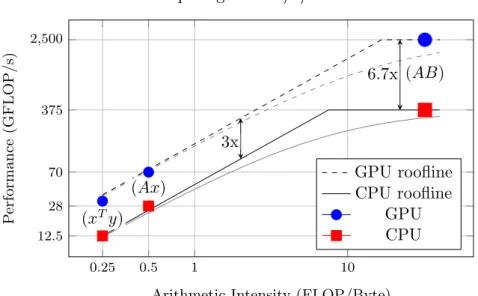
In order to build a roofline model to compare CPU and GPU performance, we construct the model using measured performance numbers from benchmark-ing BLAS1, BLAS2, and BLAS3 vector and matrix operations. In Fig. 2.1 we compare an 8-core Intel E5-2670 processor and an NVIDIA K20x GPU, and use Intel’s highly tuned MKL BLAS library, and NVIDIA’s CUBLAS library, to imple-ment single-precision dot product (xTy) (BLAS1), matrix-vector multiplication (Ax) (BLAS2), and matrix multiplication (AB) (BLAS3), such that matrix-matrix multiplication becomes our “peak” floating point performance. Memory bandwidth was measured using an adapted version of the STREAM3
benchmark-ing code and was around 150 GB/s (with ECC on) for the K20x and around 50 GB/s for the CPU.
As can be seen and expected, the speedup is close to 3x for the lower arith-metic intensity BLAS1 and BLAS2 operations follow the bandwidth curves. For large matrix-matrix multiplication, we expect and achieve greater final speedup of 6.7x, which fits the ratio between NVIDIA’s and Intel’s published theoretical peak performance. Thus, if our algorithm can be structured to take advantage of cache and achieve a relatively high arithmetic intensity, we can achieve a GPU speedup between 3x and 7x (relative to 8 cores). However, as most supercom-puting CPU nodes have two 8-core CPUs (compared to only a single GPU) a more realistic speedup4 is 2x–4x to provide a more realistic evaluation. Of course this
3https://www.cs.virginia.edu/stream
0.25 0.5 1 10 12.5 28 70 375 2,500 3x 6.7x (xTy) (Ax) (AB)
Arithmetic Intensity (FLOP/Byte)
P
erformance
(GFLOP/s)
Roofline comparing BLAS1/2/3 for GPU and CPU
GPU roofline CPU roofline
GPU CPU
Figure 2.1. Exact roofline model (2.1) and first-order approximation (2.2) com-parison between BLAS1, BLAS2, and BLAS3 operations on a single K20x GPU vs. an 8-core Intel CPU using the highly tuned linear algebra libraries CUBLAS and Intel MKL.
assumes that both the GPU and CPU versions run a similarly well-optimized ver-sion of the same algorithm.
2.2.2
CUDA programming model
Many codes looking to add performance via GPUs are written in Fortran or C/C++ and utilize MPI for both intranode and internode parallelization. In order to push into the area of multicore and many-core architectures, some codes are exploring shared memory threading for intranode parallelism in or-der to reduce the communications load resulting from too many MPI processes. On the CPU side, we see OpenMP as the dominant threading backend, for both multicore CPUs and the new many-core Xeon Phi (MIC) from Intel.
The CUDA programming model exposes the GPU as a shared memory massively-threaded computing device, and in contrast to OpenMP, the CUDA C language is a superset of the C language as opposed to a set of compiler directives. CUDA allows the programmer to specify functions that should execute on the GPU called kernels. CUDA includes additional syntax, for both kernel specification and launch on the GPU, using any number of desired threads.
In a typical CPU shared-memory data parallel application, a threading model like OpenMP is used to parallelize a loop, where the iterations are independent. Output variables and arrays where reduction operations can occur require spe-cial care using atomic operations or locking mechanisms. To achieve the best performance, most programmers maintain a mental model of the loop itera-tions, and how the work is being split across CPU threads. We see a very small abbreviated example implementation using OpenMP (left) and CUDA (right) of the operation~z ← a~x + ~y in Fig. 2.2.
// OpenMP parallelization
void saxpy_cpu(a,x,y,z)
#pragma omp parallel for
for(int i=0; i<N; i++) z[i] = a*x[i] + y[i];
// CUDA Kernel
__global__ void saxpy_kernel(a,x,y,z)
int id = threadIdx.x
+ blockIdx.x*blockDim.x; z[id] = a*x[id] + y[id];
Figure 2.2. Abbreviated C-code comparing OpenMP and CUDA implementa-tions of~z ← a~x + ~y.
The CUDA GPU programming model, when framed in terms of threading a looping construct, is remarkably similar. The major difference is that CUDA is
always parallel and the loop keywords (e.g., for(;;)) are never actually writ-ten. Generally the body of the loop is written as a function of the loop index (in this case id), where one thread is launched per loop index and identified using the thread unique structures threadIdxandblockIdx. These threads, in contrast to CPU threads, are very lightweight and work in teams called blocks and are scheduled in groups called “warps.” These warps work together to coa-lesce memory transfers and cache access. Ensuring that variables are organized to take advantage of the warp collective access patterns is critical to performant GPU code. Additionally, as in OpenMP or any shared-memory threading model, CUDA kernels must also take care to avoid race conditions, an important perfor-mance consideration we will see in an upcoming section.
2.2.3
Related work
Within a few years of the release of CUDA, many groups began to experiment with GPUs for scientific and numerical work, many especially interested in the simulation of PDEs, especially for hyperbolic problems such as wave propaga-tion. Klöckner et al.[2009] demonstrated a newly developed higher-order dis-continuous Galerkin (DG) GPU code simulating Maxwell’s equations. Compar-ing a sCompar-ingle CPU against a sCompar-ingle consumer GPU, they managed a speedup of
65x. However, an experiment conducted using supercomputing resources (of that time) would have pitted a single GPU (of similar performance) against two quad-core CPUs. Assuming perfect CPU scaling, we would have seen a speedup closer to 8x, which suggests that this implementation of higher-order (discontin-uous) finite elements yields more than the expected speedup and that the CPU version was less than optimal.
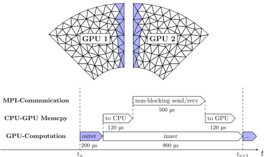
More recently, the HPC world has seen larger-scale GPU cluster installations and corresponding simulations, such as work presented by Shimokawabe et al. [2011]. Running on Japan’s TSUBAME 2.0 cluster with 4,000 GPUs (and 16,000 CPU cores), they ran a “dendritic solidification” simulation that achieved just over 1 PFLOP/s of single-precision performance using the full cluster. Although different than the hyperbolic PDE models we are interested in solving, the PDE model consists of separated spatial and temporal differential operators, allowing finite differencing in space and an explicit time-stepping scheme in time to be used. A traditional parallelization method is used, where the physical domain (a finite difference grid) is partitioned across GPUs. However, in an attempt to utilize the CPUs on each node, they compute these halo-region elements using the CPUs in parallel with the “inner” grid elements on the GPU. The MPI mes-sages are sent by the CPUs as it completes the top, bottom, back, front, left, and right faces. Thus, this approach can utilize the full compute power of the system, CPUs+ GPUs, where many GPU simulations (including SPECFEM3D) leave the CPUs essentially idle, used only to control the GPU simulations and manage I/O for MPI and disk operations.
Finally, we consider the SEISSOL software package [Dumbser and Käser, 2006]. Providing a similar set of features to the SPECFEM3D package, it sim-ulates the elastic wave equation on unstructured finite-element meshes. It ad-ditionally provides a form of local time stepping [Dumbser et al., 2007] (de-veloped for SPECFEM3D in Ch. 3). In contrast to the continuous finite-element spatial discretization employed by SPECFEM3D, SEISSOL utilizes a DG finite-element method, which has several advantages and disadvantages. Because the finite-element polynomials are discontinuous at each element boundary, the mass matrix M is block diagonal, where each element’s block in the matrix is fully uncoupled from the others. Thus, it is no longer necessary to employ the use of Gauss–Lobatto–Legendre (GLL) collocation points and Gaussian quadra-ture[Komatitsch et al., 2003] to achieve the efficient computation of M−1(trivial in SPECFEM3D because M is diagonal). This allows the use of both hexahedral and tetrahedral elements, where tetrahedra are generally far easier to use from a mesh-generation perspective. This additional flexibility can be a big advantage, depending on the particular use. However, the duplicated degrees of freedom
at each element boundary come with a computational cost, and SEISSOL was known to be less efficient than SPECFEM3D, although it is difficult to find an exacting comparison between the two.
Recently, Heinecke et al.[2014] detailed the optimization and extension of SEISSOL to work using Intel’s XEON Phi (MIC) accelerator modules, which are Intel’s response to GPU computing and have many similarities from an architec-tural perspective, including a large number (60+) of relatively simple processors with wide vector units and high bandwidth GDDR5 memory. Experiments run on the Tianhe-2 supercomputer (world’s fastest as of November 2014 and largest Intel MIC cluster installation) with three Intel MIC accelerators in each of the 8192 nodes, was able to achieve up to 8.6 PFLOP/s of double-precision perfor-mance in weak-scaling benchmarks. SEISSOL follows a similar parallel structure to SPECFEM3D (see Sec. 2.4), where partition boundaries are computed first in order to allow the MPI communications to run concurrently with the “inner” nonboundary element updates.
2.3
SPECFEM3D GPU
The initial excitement about the potential performance of GPUs prompted Ko-matitsch et al.[2010] to port a limited version of the SPECFEM3D forward solver to GPUs. They showed a speedup of 13x using a single NVIDIA Tesla S1070 against a 4-core Intel “Nehalem” CPU — far less than the incredible speedups in some fields, but a promising result nonetheless. This limited code, however, was not meant to be used in production, and would require significant effort to extend for use in seismic imaging.
In order to reevaluate the code on the newest GPU clusters and extend the functionality to include the additional routines necessary for adjoint tomogra-phy, we decided to add GPU functionality to the SPECFEM3D 2.0 “Sesame” [Peter et al., 2011] software package (via a GPU_MODE logical). We were able to reintegrate the stiffness matrix and time-stepping GPU kernels, but the GPU initialization and extensions for adjoint tomography were additionally ported to CUDA using the CPU version as a reference. Although this added additional complexity to the original code, using the structure of the CPU version to stage the GPU computations makes both testing and maintenance much simpler.
We choose to use CUDA as the GPU programming language and environ-ment, given its maturity, stability, and ubiquity at the time of development.5 The
5Mixing CUDA-C and Fortran did, however, create a lot of off-by-one bugs due to their array indexing differences.
rise of semiautomatic schemes using accelerator directives, such as OpenACC, seems to be an excellent compromise, but were seen as too immature at the time of development. Additionally, they can make use of NVIDIA’s additional profiling and developer tools more difficult. It is also unlikely that one could port the en-tire SPECFEM3D code to GPUs via OpenACC and expect excellent performance; however, a hybrid approach may provide the shortest time-to-solution in terms of development costs. By initially annotating the entire time-stepping loop with OpenACC directives, the initial GPU version can be built and tested with relative confidence. By profiling, we can determine the most complex routines which can be rewritten by hand using CUDA, saving a lot of development effort for the many simpler code paths, such as time stepping, absorbing boundaries, and simple source mechanisms, which are simple enough for an OpenACC compiler. We might also consider semiautomated CUDA compilers such as PyCUDA which was developed by Klöckner et al. [2012]. This unique CUDA framework allows the generation of (optimized) CUDA kernels from within a simplified Python DSL. The use of Python in science via NumPy and SciPy has grown rapidly, and provides compelling competition for native Fortran or C++ CUDA developement due to Python’s ease of use and extensive and high-quality sci-entific and numerical library ecosystem. PyCUDA uses C-code generation tech-niques to provide high-performance CUDA kernels; however, it is hoped that NVIDIA’s release of an LLVM6→ PTX7 library will allow many more tools similar
to PyCUDA that make GPU programming drastically easier. Holk et al. [2013] already presented a proof of this concept via the Rust8 language and compiler,
which uses LLVM as its intermediate representation (IR) and optimizing back-end. With only a few modifications and the addition of several keywords, they were able to write CUDA kernels in Rust that were compiled into native CUDA kernels with performance comparable to writing them in CUDA C.
2.3.1
The spectral element method for GPUs
Having introduced the CUDA programming model, we can introduce how we implemented our particular choice of spatial discretization for applications in seismology. SPECFEM3D implements the spectral element method (SEM), which is a carefully constructed finite-element method that provides a flexible and
ef-6LLVM is a general-purpose intermediate representation and backend for compiler authors (www.llvm.org)
7PTX is a GPU-specific intermediate representation for NVIDIA GPUs
8A new systems language with a focus on memory safety, concurrency, and performance (http://www.rust-lang.org).
ficient spatial discretization for wave-propagation modeling. More specifically, we are interested in discretizing the elastic wave equation on some 3D domain x∈ Ω,
ρ(x)∂
2u
∂ t2 − ∇ · T(x, t) = f (xs, t) , (2.3)
T(x, t) = C(x) : ∇u(x, t) , (2.4)
where ρ(x) is the material density, C is the forth-order elasticity tensor with 21 independent parameters in the fully anisotropic case and f(xs, t) represents the forcing caused by e.g., an earthquake, commonly modeled as a point source at xs. Additionally, for well-posedness, this equation requires appropriate initial and boundary conditions. In order to motivate the structure of the code, and associated computational costs, we present an abbreviated outline of the SEM applied to (2.3), which can be seen in far greater detail from the original cre-ators of SPECFEM3D, Komatitsch and Tromp [2002]; Tromp et al. [2008], and from Canuto et al.[2006].
Following a standard Galerkin finite-element procedure we multiply this equa-tion by a test funcequa-tion w and integrate by parts over the domainΩ to obtain the weak formulation Z Ω w· ρ(x)∂ 2u ∂ t2 = Z ∂ Ω ˆn · T · w dS − Z Ω ∇w : T dΩ + Z Ω w· f (xs, t) dΩ. (2.5) We note that the first and third terms of this expression will yield the so-called
mass and stiffness matrices. The second term, an integral over the domain’s boundary surfaces, is typically modeled as zero on the free surface, and is re-formulated on the artificial domain boundaries as an (approximate) absorbing boundary condition. The final term including the source, is generally localized to a single element, although we will consider an application with a fault source in Sec. 4.3.6.
We begin the discretization process by representing the 3D domainΩ with a set of nonoverlapping hexahedral elementsΩk to make up our discrete domain such that
K [ k=1
Ωk= Ωh.
We further restrict the space of w to a finite set of polynomials φ(x, y, z) each with compact support in each element Ωk. To simplify defining the method, consider a reference element defined by the variables −1 ≤ ξ, η, ζ ≤ 1. For the
SEM, we choose our polynomials as the set of Lagrange polynomials defined by `j(ξ) = Y 0≤m≤N m6= j ξ − ξm ξj− ξm = (ξ − ξ0) (ξj− ξ0) · · · (ξ − ξj−1) (ξj− ξj−1) (ξ − ξj+1) (ξj− ξj+1)· · · (ξ − ξk) (ξj− ξk) for 0≤ j ≤ N , where we note that `j(ξj) = 1 and `j(ξi6= j) = 0. If we consider
a function f(x), we represent it using the following approximation using triple products of these Lagrange polynomials
f(x(ξ, η, ζ)) ≈
Ni,Nj,Nk
X i, j,k=0
fi, j,k`i(ξ)`j(η)`k(ζ).
where fi, j,k= f (x(ξi,ηj,ζk)). Critical to the SEM, we choose our set of (ξi,ηj,ζk) to be the well-known GLL collocation points, which when combined with these Lagrange polynomials and the GLL quadrature rule, simplify the evaluation of the integrals in the weak formulation and critically yield a diagonal mass matrix allowing for explicit time-stepping schemes.
In order to solve the weak form (2.5) using our reduced set of test functions, we utilize the GLL quadrature such that the following integral approximation on an element Ωe retains the convergence properties of a standard finite-element method Z Ωe f(x) dΩ = Z Ωref f(x(ξ, η, ζ)) J(ξ, η, ζ) dΩref (2.6) ≈ Ni,Nj,Nk X i, j,k=0 ωiωjωkfi, j,kJi, j,k (2.7)
where ωi, j,k represent the GLL quadrature rules and J(ξ, η, ζ) represents the
integral mapping between the reference element Ωref and the original element Ωe. With the integral rule defined, we can apply this to our original weak form. The first term in the weak form (2.5), after integration, becomes the so-called
mass matrix. We can rewrite this term with respect to a single elementΩe and the reference element Ωref, and with the application of (2.6), we get the final spatially discrete form
Z Ωe w· ρ(x)∂ 2u ∂ t2dΩ = Z Ωref ρ(x(ξ))w(x(ξ)) · ∂ 2u(x(ξ)) ∂ t2 J(ξ) dΩref ≈ Ni,Nj,Nk X i, j,k=0 ωiωjωkJi, j,kρi, j,k 3 X m=1 w(m)i, j,k∂ 2u(m) i, j,k ∂ t2 (2.8)
Following the Galerkin finite-element method, we choose wi, j,k= `i, j,k(ξ), each
of which is nonzero only at a single GLL colocation point, that is, w(m)can be cho-sen to be independently zero, creating independent expressions for each com-ponent of u. Critically, this resulting set of expressions is assembled (in the finite-element sense) into the diagonal matrix M, allowing the use of explicit time-stepping schemes for time-discretization.
Continuing this abbreviated SEM introduction, we move to the most complex term, which includes the linear elasticity tensor. This yields the stiffness matrix, the most expensive operator we will derive. To start we rewrite the stiffness integrand in terms of its inner product terms
∇w : T = 3 X i,k=1 Fik∂ wi ∂ ξk , (2.9) where Fik= 3 X j=1 Ti j∂jξk, Fikαβγ= Fik(x(ξα,ηβ,ζγ)), (2.10) recalling the second-order stress tensor T (9 terms) and the ξk terms from the inverse Jacobian, which requires that no mesh elements yield a singular Jacobian (a typical finite-element requirement). In order to evaluate the integral, we need this tensor evaluated at each of the element GLL points
T(x(ξi,ηj,ζk)) = C(x(ξi,ηj,ζk)) : ∇s(x(ξi,ηj,ζk)).
Recalling the integral for the stiffness term, we apply the quadrature rule and rearrange terms to produce the stiffness approximation
Z Ωe ∇w : T dΩ = 3 X i,k=1 Z Ωe Fik∂ wi ∂ ξk ≈ Nα,Nβ,Nγ X α,β,γ=0 3 X i=1 wαβγi × ωβωγ Nα X α0=0 ωα0Jα 0βγ Fiα10βγ`0α(ξα0) (2.11) + ωαωγ Nβ X β0=0 ωβ0Jαβ 0γ Fiαβ2 0γ`0β(ξβ0) +ωαωβ Nγ X γ0=0 ωγ0Jαβγ 0 Fiαβγ3 0`0γ(ξγ0) ,
where `0i = dξd`(ξi) is a result of evaluating ∇w. As with the mass-matrix eval-uation, the wαβγi are the set of Lagrange polynomials, independently zero, such that both sums (over α, β, γ, and i) drop all but a single term, separating the degrees of freedom. Thus, each row of the stiffness matrix K, indexed byα, β, γ is defined by the similarly indexed expression in (2.11) containing the degrees of freedom within that element Ωe. Additionally, the expressions for rows that correspond to nodes on an element-element boundary, contain terms from all neighboring elements, a process well known as assembly.
Ignoring the boundary and forcing terms, we can write this system as M d 2 d t2 ux uy uz +K ux uy uz =0 (2.12)
or, more simply,
M¨u+ Ku = 0, (2.13)
where the matrices M and K are filled by the appropriate terms from (2.8) and (2.11). Furthermore, M is diagonal, and K is extremely sparse, with each row only containing nonzero entries corresponding to degrees of freedom that are shared by the element or elements that contain the row’s respective node. Time discretization
The matrix equation (2.13) is finally ready for a time-discretization scheme and, because the mass matrix is diagonal, we can rewrite the system simply as
¨
u= −M−1Ku
because M−1 is trivially computable. This form with derivatives of u on the left, and linear functions of u on the right, allows for the use of explicit time-stepping schemes. Although many schemes are possible, SPECFEM3D currently utilizes the well-known explicit Newmark time-stepping scheme[Krenk, 2006]. A second-order accurate scheme that conserves a discrete quantity (a perturba-tion of the discrete energy), it can be written as
un+1= un+ ∆t vn+ ∆t2 2 an, vn+1/2= vn+ ∆t 2 an, an+1= −M−1K un+1, vn+1= vn+1/2+∆t 2 an+1.
As can be quickly observed, these time-stepping operations require only vector arithmetic (e.g., un+ ∆t vn), with the exception of the computation of K un+1.
Furthermore, these simple vector operations are at the mercy of the memory bandwidth with little room for optimization, whether that is on a standard CPU or a multithreaded GPU.
2.3.2
SEM computational structure
One advantage of the explicit Newmark time-stepping scheme shown in the last section is its ability to compute updates in place, that is no additional memory is required beyond the field variables u, v, a. The SPECFEM3D CPU and GPU code both follow the same basic computational sequence seen in Alg. 1.
Algorithm 1 Newmark time stepping for SEM. Require: u= u0, v= v0, a= ~0, ∆t, source term S.
1: for tn= 0, . . . , Tn do 2: u← u + ∆t v +∆t22a 3: v← v +∆t2 a 4: a← ~0 5: a← Ku + S 6: a← −M−1a 7: v← v +∆t2 a 8: end for
Besides the stiffness matrix operation Ku in step 5, these steps offer only the low arithmetic intensity of BLAS1 operations, which we’ve seen to offer only modest speedup opportunities for a GPU, on par with the approximate 3x mem-ory bandwidth gap between a GPU and multicore CPU. The computation of Ku, on the other hand, represents a higher arithmetic intensity and thus offers addi-tional opportunities to take advantage of the higher peak floating point perfor-mance of the GPU.
Stiffness matrix computation
Although there exist efficient sparse-matrix vector multiplication libraries for both CPUs and GPUs, because we know the exact structure of K, it is more efficient to implement this operation implicitly as the action of K onto u. Recall the computation ofRΩ
e∇w : T dΩ (2.11) that is split into four sums over element
function wαβγi isolates all but the following terms for each index corresponding to a node in each element (or a row in K) allowing us to define a function
k(Ωe,α, β, γ) that computes the contribution to each value of a for each element Ωe and nodeα, β, γ: k(Ωe,α, β, γ) =ωβωγ Nα X α0=0 ωα0Jα 0βγ Fiα10βγ`0α(ξα0) +ωαωγ Nβ X β0=0 ωβ0Jαβ 0γ Fiαβ2 0γ`0β(ξβ0) (2.14) +ωαωβ Nγ X γ0=0 ωγ0Jαβγ 0 Fiαβγ3 0`0γ(ξγ0).
In this expression, the field variables u defined at each node are embedded within the computation of Fi jαβγ. However, in this expression, only values of u de-fined within the element contribute, allowing the computation to be structured by element. In fact, the CPU version of SPECFEM3D organizes the updates to a as a loop over elements containing a loop over element nodes, the body of which contains the computation of (2.14).
Each of the entries in u, v and a corresponds to an element node, some of which are shared between elements. To solve this sharing problem, each en-try is given a global index and is referenced using a technique known as
indi-rect addressing to map element-local nodes to these global degrees of freedom. This structure yields Alg. 2 outlining the structure of the computation of Ku in SPECFEM3D.
Algorithm 2 CPU Ku computation in SPECFEM3D.
1: for allΩe∈ Ωh do
2: for allα, β, γ ∈ Nα, Nβ, Nγ do
3: element-node contribution← k(Ωe,α, β, γ)
4: iglobal← global-lookup(Ωe,α, β, γ)
5: a(iglobal) ← a(iglobal) + element-node contribution
6: end for
7: end for
We note that the function k(Ωe,α, β, γ) embeds a similar global lookup for
u, and that the in-place sum operation in line 5 is a result of the required finite-element assembly due to shared nodes on element boundaries (multiple
elements contain nodes with identical iglobal index values). This choice of CPU
implementation drives the mapping to the GPU programming model.
As noted in Sec. 2.2.2, the CUDA threading model exposes and organizes itself in terms of lightweight threads organized in teams called blocks. We choose the natural mapping, where the loop over elements is mapped to CUDA blocks, and the loop of nodes is mapped to CUDA threads. The CUDA kernel is written as the body of these loops with the CUDA runtime launching and scheduling the necessary blocks and threads running on each kernel instantiation, outlined in Alg. 3
Algorithm 3 GPU Ku computation kernel in SPECFEM3D
1: Ωe← blockId 2: α, β, γ ←threadId
3: element-node contribution← k(Ωe,α, β, γ)
4: iglobal← global-lookup(Ωe,α, β, γ)
5: a(iglobal) ← a(iglobal) + element-node contribution
This mapping of blocks to elements and threads to nodes was done in the original GPU implementation by Komatitsch et al. [2010], but is supported by analysis done by Cecka et al. [2011] and is additionally used by the high-performance DG code for Maxwell’s equations in [Klöckner et al., 2009]. With the structure of the kernel set, there are a number of key optimizations, which are critical to the performance of the GPU version, which we outline in the next section.
2.4
GPU performance optimizations
Ensuring that the GPU version achieves high performance is critical, due to the high programming and maintenance costs relative to a CPU version. We high-light some of the most critical optimizations including
1. shared-memory caching,
2. fast and correct updates to shared degrees of freedom, 3. optimizing memory operations,
The previous section introduced the SEM for elastic wave propagation, in-cluding the most expensive operation a ← Ku which accounts for more than 65% of runtime. As noted, blocks are mapped to elements, and threads to nodes. SPECFEM3D commonly uses fourth-order finite-element polynomials, which leads to Nα × Nβ × Nγ = 125 nodes per hexahedral element, conve-niently close to 128. The GPU internally schedules threads in groups of 32 called “warps,” such that when possible, structuring computations around factors of 32 generally produces the highest performance. In the next section we detail the structure of the kernel, including managing cache by hand.
Shared memory: explicit caching
GPUs, unlike CPUs, require explicit management of cache by making use of explicitly allocated shared memory denoted by the __shared__ variable pre-fix. This shared memory is actually on-chip and has near register access speeds (about 40 cycles[Volkov and Demmel, 2008; Wong et al., 2010]) and is visible to all threads within a block. A common CUDA development pattern has each thread fetching a corresponding common value from global memory and storing it in the shared memory cache, followed by the __syncthreads()barrier. The function k(Ωe,α, β, γ) from (2.14) can take advantage of shared memory as cer-tain variables are reused across nodes (and threads). We outline this in Alg. 4 detailing the structure of the CUDA implementation.
Algorithm 4 GPU Kernel Ku outlining use of shared memory cache. Require: __shared__ float shared_u[NαNβNγ],shared_JF[NαNβNγ]
1: Ωe← blockId 2: α, β, γ ←threadId
3: iglobal← global-lookup(Ωe,α, β, γ)
4: shared_ux, y,z[threadId]← ux, y,z(iglobal)
5: __syncthreads()
6: shared_JF(x,y,z),j[threadId]← J(x,y,z),jα,β,γ (Ωe)F(x,y,z),jα,β,γ (shared_ux, y,z) 7: __syncthreads()
8: ax, y,z(iglobal) ← ax, y,z(iglobal) +
9: ωβωγPNαα0=1ωα0`0α(ξα0)shared_JF(x,y,z),1(α0,β, γ) +
10: ωαωγPNββ0=1ωβ0`0β(ξβ0)shared_JF(x,y,z),2(α, β0,γ) +
11: ωαωβPNγ0γ=1ωγ0`0γ(ξγ0)shared_JF(x,y,z),3(α, β, γ0)