HAL Id: hal-00016814
https://hal.archives-ouvertes.fr/hal-00016814
Submitted on 11 Jan 2006
HAL is a multi-disciplinary open access
archive for the deposit and dissemination of sci-entific research documents, whether they are pub-lished or not. The documents may come from teaching and research institutions in France or abroad, or from public or private research centers.
L’archive ouverte pluridisciplinaire HAL, est destinée au dépôt et à la diffusion de documents scientifiques de niveau recherche, publiés ou non, émanant des établissements d’enseignement et de recherche français ou étrangers, des laboratoires publics ou privés.
Relevance of Massively Distributed Explorations of the
Internet Topology: Qualitative Results
Jean-Loup Guillaume, Matthieu Latapy, Damien Magoni
To cite this version:
Jean-Loup Guillaume, Matthieu Latapy, Damien Magoni. Relevance of Massively Distributed Explo-rations of the Internet Topology: Qualitative Results. Computer Networks, Elsevier, 2006, 50 (16), pp.3197-3224. �10.1016/j.comnet.2005.12.010�. �hal-00016814�
Relevance of Massively
Distributed Explorations
of the Internet Topology:
Qualitative Results
1 Jean-Loup Guillaume2, Matthieu Latapy2and Damien Magoni3
Abstract—Internet maps are generally constructed using the traceroutetool from a few sources to many desti-nations. It appeared recently that this exploration process gives a partial and biased view of the real topology, which leads to the idea of increasing the number of sources to im-prove the quality of the maps. In this paper, we present a set of experiments we have conducted to evaluate the relevance of this approach. It appears that the statistical properties of the underlying network have a strong influence on the quality of the obtained maps, which can be improved using massively distributed explorations. Conversely, some statis-tical properties are very robust, and so the known values for the Internet may be considered as reliable. We validate our analysis using real-world data and experiments, and we discuss its implications.
Index Terms— Internet topology, graphs, metrology, ac-tive measurements.
INTRODUCTION.
Due to its fully distributed construction and ad-ministration, mapping the Internet (in terms of IP routers and IP-level links between them) is a chal-lenging task. It is however essential to obtain some information on its global shape. Indeed, it plays a central role in key problems like network robustness, see for instance [43], [4], [14], [15], simulation of future protocols and uses, see for instance [41], and many others.
Exploring the Internet topology is a research prob-lem in itself, see for instance [26], [28], [39], [57], [62]. Indeed, many difficulties (like the identifica-tion of the multiple interfaces of a same router) arise when one wants to map the Internet. Various tech-niques and methods have been introduced to achieve
1
A reduced conference version of this contribution [32] has been
accepted for publication in the proceedings of the 24-thIEEE
interna-tional conference INFOCOM, 2005.
2
LIAFA–CNRS– Universit´e Paris 7 – 2 place Jussieu, 75005 Paris, France. (guillaume,latapy)@liafa.jussieu.fr
3
LSIIT–CNRS– Universit´e Strasbourg 1 – UFR de Math-Info – 7, rue Ren´e Descartes F-67084 Strasbourg, France
this goal. Some of them are very subtle, but cur-rent explorations still rely on the extensive use of the traceroutetool: one collects routes from a given set of sources to a given set of destinations, and then merges the obtained paths. Some post-processing is generally necessary to clean the obtained data, but we do not enter in these details here.
Two points are particularly important in the scheme sketched above. First, it must be clear that the image we obtain from the network is partial (ex-cept if the number of sources and destinations is huge, we certainly miss some nodes and some links) and may be biased by the exploration process (some properties of the obtained map may be induced by the way we explore the network, not by the network itself). Second, the number of sources cannot be in-creased easily, whereas one can take as many desti-nation as one wants. Indeed, one needs direct access to the sources in order to run thetraceroutetool, whereas one only needs theIPaddresses of the desti-nations. In the case of [26] for instance, which is one of the largest explorations currently available, only a few dozens of sources are used whereas there are several hundreds of thousands destinations.
Recently, several researchers conducted experi-mental and formal studies to evaluate the accuracy of the obtained maps of the Internet [1], [13], [17], [18], [31], [32], [33], [35], [52], [56]. All these studies use simple models of networks and traceroute but they all give good arguments of the fact that the cur-rently available maps of the Internet are very incom-plete, and that there probably is an important bias induced by the exploration process.
In order to improve these maps, several re-searchers and groups now propose to deploy mas-sively distributed measurement tools [25], [53], [55]. The basic idea is that dramatically increasing the number of sources would significantly improve the quality of the obtained maps. Our central aim in this paper is to rigorously evaluate the relevance of this approach.
To achieve this, we conduct an extensive set of ex-periments designed as follows, according to the nat-ural methodology already used for instance in [13], [31], [35]. We consider a graphG representing the
network to explore. We then simulate the exploration process and obtain this way a (partial and biased) viewG′
of the original graph. We then compareG′
andG to evaluate the quality of this view. We
sources and destinations, which makes it possible to study the impact of these numbers on the accuracy of the obtained view. Likewise, we take a variety of graphs as models of the network, with very different properties, in order to investigate their influence on the exploration process and how much this process is able to capture them. We also study an important real-world data set which makes it possible to evalu-ate the relevance of the simulations.
The paper is organized as follows. First we define the statistical properties of networks relevant to our study, we present the models we use and discuss our methodology (Section I). Then we present and ana-lyze the results of our simulations on various mod-els and statistical properties (Sections II–IV). We show how our approach can be used to design effi-cient exploration strategies by choosing appropriate sources and destinations in Section VI. Section VII is devoted to the comparison of our results with real-world data and experiments, which makes it possible to identify the most meaningful simulations and to evaluate our hypotheses. Finally we present our con-clusions and discuss them.
I. PRELIMINARIES.
A network topology can naturally be represented by a graph. For our purpose, the graph does not need to be weighted nor directed. A route in the network, as given by thetraceroutetool, is a path in the corresponding graph. For a few years, a strong ef-fort has been made to discover the topology of the Internet at IP and/or router level by extensive use of traceroute and other tools (BGP tables, source routing, etc). See for instance [12], [24], [26], [50].
The obtained maps give much information on the global shape of the Internet. In particular, they gave evidence of the fact that the Internet topology has some statistical properties which makes it very dif-ferent from the models used until then, see for in-stance [10], [24]. This induced an intense activity in the acquisition of such maps [26], [28], [50], in their analysis [24], [59] and in the accurate modeling of the Internet [9], [40], [63], [64]. See [51] for an in-depth survey.
Our analysis of the exploration process will be based on these statistical properties and these mod-els, which we present below. We also need to model thetraceroutetool and the exploration process, which we also discuss in this section. Finally, we
present our methodology, and explain how our re-sults should be read.
Statistical properties
The Internet, at router level, is composed of sev-eral millions of nodes and dozens of millions of links. LetN denote its number of nodes and M its
number of links.
It is well known, and quite intuitive, that the den-sity of the Internet graph is low: the number of exist-ing links over the number of possible ones, N ·2·M(N −1), is low. In other words, the average degree k of the
nodes (their average number of links), i.e.k = 2·MN ,
may be viewed as a constant independent of the size of the network.
A less known point is that the average distance (length of a shortest path between two nodes) is low. It typically scales as log(N). This is however not
surprising, since it is an essential objective of the de-sign of the network, and since it is actually very nat-ural for any graph with some amount of randomness to have a low average distance, see for instance [8], [37], [48]. In some specific cases, the average dis-tance can even scale aslog log(N) or be bounded by
a constant independent ofn [11], [60], [61], [49].
On the contrary, although it is now well under-stood, the fact that the degree distribution of the In-ternet graph is very heterogeneous has been a sur-prise [24]. Indeed, the proportion pk of nodes of
degree k might be approximated by a power of k: pk ∼ k
−α
withα ≃ 2.5. Intuitively, this means that
most nodes have a low degree but there exists some nodes with (very) high degree. Such graphs are said to be scale-free.
Another important statistical property measured on the Internet is its clusteringC defined as C = N∆
N∨,
where N∆ is the number of triangles (three nodes with three links) in the network andN∨ is the
num-ber of connected triples (three nodes with at least two links)4. In other words,C is the probability that
two nodes are connected together, given that they are both connected to a same third, which gives a mea-sure of the local density of the graph. The clustering of the Internet is high, considered as a constant inde-pendent ofN.
4
There are several definitions for the notion of clustering coefficient, which all have their own advantages and drawbacks. They are all aimed at capturing the local density of graphs, and would serve our purpose equivalently.
Modeling networks
The basic model for networks is the Erdos and R´enyi (ER) random graph model [8], [22]. In an ER graph withn nodes, each of then·(n−1)2 possible links exists with a given probability p. Equivalently, an
ER graph is constructed from n nodes by choosing m = p · n·(n−1)2 links at random. Notice that an ER graph contains a giant component as soon as the aver-age degree is greater than1 [8]. In the following this
condition is always fulfilled and generally the graph itself is fully connected.
In such a graph, the average distance grows as
log(n) [8] as long as p is high enough. However, the
clustering is small (it tends to zero when n grows),
and the degree distribution follows a Poisson law (pk ∼ e
−α αk
k!). This implies in particular that all
the nodes have a degree close to the average. There-fore, although this model can be considered as rel-evant concerning the average distance, it misses the two other main properties of the Internet.
An important step was made when Albert and Barab´asi (AB) introduced their model based on
pref-erential attachment [2], [20]. In this model, nodes
arrive one by one and choose k neighbors among
the existing ones with a probability proportional to their degree. The degree distribution of the nodes in the obtained graphs follow a power-law with an exponent−3 (it is possible to modify this exponent
in others models using preferential attachment). The average distance of such a graph is logarithmic in the number of nodes, but the clustering is low.
This model has been modified to give highly clus-terized graphs: in the Dorogovtsev and Mendes (DM) model [19], nodes arrive one by one but at each step one chooses a random link {u, v} and the new
node is linked to both u and v. This implies that a
node is chosen with a probability proportional to its degree. Therefore, the preferential attachment prin-ciple is hidden in this model, which induces the fact that DM graphs have a power-law degree distribu-tion. Moreover, since one forms a triangle at each step, they have a high clustering.
It is also possible to sample a random graph with a prescribed degree distribution using the Molloy and Reed5 (MR) model [38], [46], [47]. This gives
5
Despite it has been introduced in [6] and studied by Bollobas in [7], this model is commonly refferred to as the Molloy and Reed model since these authors made it popular in their contributions [46], [47]. We will follow this convention here.
Model Density Distance Degree Clustering
ER YES YES NO NO
AB YES YES YES NO
MR YES YES YES NO
DM YES YES YES YES
GL YES YES YES YES
TABLE I
CHARACTERISTICS OF THE MODELS WE USE IN THIS PAPER CONCERNING THE MAIN STATISTICAL PROPERTIES.
graphs with exactly the wanted degree distribution, but with low clustering. [7], [38], [46], [47].
Finally, the Guillaume and Latapy (GL) model [29], [30], based on bipartite graphs, gives graphs with power law degree distributions and high cluster-ing, by sampling graphs with prescribed distribution of clique (complete sub-graph) sizes.
The performance of these models are summarized in Table I. They are currently the most widely used for the realistic modeling of clusterized scale-free networks and have all their own advantages and drawbacks. In particular, the parameters are differ-ent from one model to another: the main parameter for ER and AB models is the average degree, and the others properties of these models (the degree dis-tribution for instance) are consequences of the con-struction process itself. Likewise, the original DM model has no parameter but the size of the generated graph and once again, the properties of this model are contained in the construction process. Finally, MR and GL models are defined using the degree distribu-tions one wants to obtain, and most of the properties (including the average degree) are consequences of these distributions. Therefore, depending on the tar-geted property (degree distribution, clustering, etc), one will use one model rather than another.
These models have been considered as building blocks for more complex models. See [3], [9], [19], [23], [34], [45], [51], [58], [63] for a description of some of these.
In the results we present here, our aim is to give evidence of the impact of the network properties on the efficiency of a shortest-paths based exploration. In most cases, the results do not vary qualitatively between the AB and the MR models on the one hand (which have a power-law degree distribution and no clustering), and between the DM and the GL ones on the other hand (both power-law degree distribution and clustering). We will therefore mainly present
results on ER, AB and DM models, except in Sec-tion VII where it is particularly relevant to use MR and GL ones.
Modelingtracerouteand the exploration
In this paper, we will make the classic assumption [13], [35] that a route as obtained bytraceroute is nothing but a shortest path between the source and the destination. It is known that this is not always true, see for instance [33], [36]. However, this choice is motivated by the two following points:
• this approximation has little influence, if any, on
our results, which we will demonstrate in Sec-tion VII,
• and realistic modeling of routes is nowadays a
challenging issue for which no better solution usable in our context is known [33], [36]. Moreover, let us emphasize on the fact that we will make an intensive use of route simulations, which makes it crucial to be able to process them very ef-ficiently. To this respect, our assumption has impor-tant advantages.
Since there may be many shortest paths between two nodes, this is not sufficient to properly define a model oftraceroute. At a given moment, the route followed by a packet when a given router routes it to a destination will always be the same indepen-dently of the sender. This may have an influence on the quality of the exploration process, therefore we included it in our model of traceroute: we al-ways follow the same shortest path (initially chosen randomly) between any two nodes. In [35] a similar model oftraceroutebased on shortest-paths has been introduced.
We now have a precise model of routes as viewed by traceroute. But we also need a model for the exploration process. We considered two points of view: in the first one we suppose that we make a snapshot of the network, and in the second one we suppose we make a long-time exploration. This leads respectively to the unique shortest path (USP) model, and to the all shortest paths (ASP) one: we either see only one route for any given source and destination, or we see all the possible ones. The ASP model should not be considered as a realistic model, since one cannot expect to get all shortest-paths even within a long period of time (in such a long time, the network is very likely to evolve). However it can be considered as a best case procedure when
dealing with shortest-paths or as an upper bound on the amount of information one can expect from a shortest-paths based exploration. The actual qual-ity of such an exploration lies somewhere in between USP and ASP.
We also conducted experiments using other mod-els (random shortest path, several shortest paths but not all, etc), and the results did not qualitatively vary, so we do not detail them here.
Finally, we generally consider a set of sources and a set of destinations, and make the exploration using each possible couple of source and destina-tion in these sets. Such a study has already been conducted on real data in [5], where the authors have defined this exploration scheme as a (k,
m)-traceroute study (the exact definition appears later in [35]), where k is the number of sources
andm the number of destinations chosen at random.
Then all tracerouteare performed between the sources and the destinations. We are going to use a similar approach in the following.
Methodology and grayscale plots
Our global approach is as follows:
1) generate a graph G using a given model with
some known properties, 2) compute a view G′
of G using a given model
of the exploration process and a set of sources and of destinations, and
3) compare the statistical properties of G′
to the ones ofG.
This methodology is very natural, and has already been used for instance in [13], [31], [35].
Let us insist on the fact that we seek qualitative results only: we want to know how qualitative prop-erties of the network influences the propprop-erties we ob-serve during an exploration process, and how reliable are the obtained maps with respect to some statistical properties. It makes no sense to interpret quantita-tively the results obtained with the kind of approach we use here. On the contrary, by the simplicity of the models and of the properties we use, we obtain evidences of the fact that some properties play a fun-damental role in the exploration whereas others may be neglected.
In the method sketched above, the third point (comparison of the original graph with the view we obtain) is a difficult task. It generally leads to a huge amount of plots which one has to compare. To help
in this, we will make an extensive use of grayscale plots which we define as follows (see Figure 8 for some easily readable examples).
For a graphG with N nodes, we consider a square
of sizeN × N. Each point (x, y) of the square
cor-responds to a view G′
of G using x sources and y
destinations with a given model of the exploration process (the point (0, 0) is in the lower left corner).
The point is drawn using a grayscale representing the value of the non-negative real-valued statistical prop-ertyp under consideration: from black for p = 0 to
white for the maximal value of p (which might be
greater than the real value).
Therefore, in these plots, the point(0, 0) is always
black (we do not see anything using zero sources and zero destinations and in this case all the proper-ties we will consider are null) and the point(N, N)
has the grayscale corresponding to the value of p
for the original graph G (when every node is a
source and a destination, we see everything: G′ = G). The points darker than the point (N, N)
corre-spond to conditions where the value of p is
under-estimated, whereas points clearer correspond to con-ditions where it is over-estimated. The gray variation is linear: if a dot is twice darker than another dot, then the associated value is twice as large.
Notice that each point of such a plot corresponds to a graphG′
, and computing such plots is computa-tionally expensive. Therefore, is it important to effi-ciently compute them and to keep N quite low. We
conducted experiments withN = 103,N = 104 and N = 105 typically, and, whereas some finite size
ef-fects are visible on small graphs (N = 103), these
ef-fects disappear for graphs of sizeN = 104and more.
This is why we will present plots for this value ofN
in general.
Finally, to improve the grayscale plots readability, we added on each such plot the0.25–, the 0.50–, the 0.75– and the 0.99–level lines, where the l–level line
is defined as the set of points where the value of p
over its maximal value is between l − 0.01 and l + 0.01. These lines are often a precious help in the
interpretation of the grayscale plots. See Figure 8 and the rest of the paper for examples.
II. PROPORTION DISCOVERED
In this section, we focus on the most basic statisti-cal properties of an exploration, namely the propor-tion of discovered nodes, the proporpropor-tion of discov-ered links, and the quality of the evaluation of the
average degree. We present the relevant results on the ER, the AB, the MR and the DM models, and we explain which parameters have a strong influence on these results.
Notice that results using similar approach have been obtained in [5], however our explorations are processed on random graphs instead of real data, the aim being to highlight the parameters of the models and therefore the characteristics of the graphs which influence the efficiency of the exploration.
All possible destinations and few sources
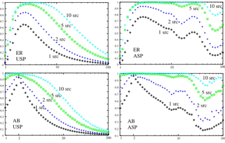
1 10 100 1 src 2 src 5 src 10 src USP ER 0 0.2 0.3 0.4 0.5 0.6 0.7 0.8 0.9 1 0.1 1 10 100 1 src 2 src 5 src 10 src ASP ER 0 0.1 0.2 0.3 0.4 0.5 0.6 0.7 0.8 0.9 1 1 2 20 200 5 src 10 src 2 src 1 src USP AB 0 0.1 0.2 0.3 0.4 0.5 0.6 0.7 0.8 0.9 1 1 2 10 src 5 src 1 src 2 src ASP AB 0.1 0.2 0.3 0.4 0.5 0.6 0.7 0.8 0.9 1 20 200
Fig. 1. Proportion of discovered links versus average degree in an
ER graph (first row) and in an AB graph (second row) when one uses a USP exploration (left column) or an ASP one (right column). Plots are given for various (small) numbers of sources (namely 1, 2, 5 and
10). All the nodes are taken as destinations. N= 104.
Let us first study what happens when the number of sources grows but stays small (all the nodes are destinations, therefore we discover all of them). We plot in Figure 1 the proportion of discovered links in several cases, as a function of the (real) average de-gree for ER and AB graphs (the only ones for which the average degree is a basic parameter). This makes it possible to check some natural intuitions: the qual-ity of the view grows with the number of sources, and it is better for ASP than for USP. Notice how-ever that as the average degree grows, the number of (shortest) paths between two given nodes grows rapidly. Therefore, the ASP exploration becomes more efficient than USP, which fails in discovering many links.
As already explained in [31], the fluctuations in the ASP plots, which may seem surprising, are due to the fact that the missed links are exactly the ones be-tween two nodes at the same distance from the source (such a link cannot be on a shortest path from the
source, and all others are). Therefore, when most nodes are at distance2 from the source (for instance
when the average degree is 69 on a 103 nodes ER
graph), many links are between them, are therefore are missed (which leads to a hole in the curve). On the opposite, when there are as many nodes at dis-tance 2 from the source as at distance 3 (typically
when the average degree is 26), then we miss only
few links (and there is a bump on the curve).
Finally, there is no significant difference between the behavior of ER and AB graphs. These plots also give evidence for the fact that, for ER and AB graphs with low average degree, only a few sources are suf-ficient if the number of destinations is large. The main reason is that with a (very) low average degree, the graph is either non-connected or nearly a tree. In this last case, the graph is obviously easy to discover. The density of the graph is therefore a first parameter which strongly influences the efficiency of an explo-ration process.
Random graphs
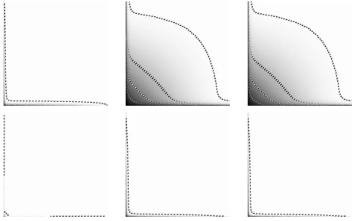
These remarks are confirmed for ER graphs by the grayscale plots in Figures 2 and 3. When the average degree is quite small, there is no qualitative differ-ence between ASP and USP (there exists in general very few shortest path between any two nodes) and the quality of the view is good even for small num-bers of sources and destinations.
Fig. 2. ER graph: number of nodes, number of links, and average
degree. k= 10, N = 104
, USP (first row) and ASP (second row).
On the contrary, when the average degree grows, so does the number of shortest paths, and the dif-ference between ASP and USP becomes significant. This can be observed in Figure 3, where we show the plots for both USP and ASP on an ER graph with high average degree. In this case, the nodes are not
harder to find than in a low-average degree graph, but the links are.
Fig. 3. ER graph: number of nodes, number of links, and average
degree. k= 100, N = 104
, USP (first row) and ASP (second row).
The fact that the average degree is obtained by di-viding two other properties which are improved by the use of more sources and/or destinations has im-portant consequences. If one of the two properties is highly biased and the other is not, then the aver-age degree will have a strong bias. The quotient acts like a worst case filter. Figure 3 shows this effect on dense ER graphs. Since the number of links is very poorly estimated, so is the average degree.
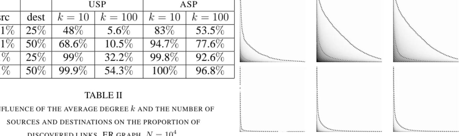
In Table II we give a few more precise values ex-tracted from the previous plots, which are of practical interest since the number of sources and destinations are small but greater than those used in current ex-ploration. Indeed, on the Internet, using only0.1%
of nodes as sources means using several thousands sources and only one recent project [53] approaches this nowadays. However, even with this number of sources, an ER graph even with a low average de-gree cannot be explored in a satisfactory way in the USP case. In order to get a nearly perfect view of the network in terms of links, one has to use at least
1% of the nodes as sources in a network with low
average degree.
Still concerning ER graphs, let us observe that, as announced, there is no qualitative difference when one changes the size of the graph: the grayscale plots for a 103 nodes ER graph (Figure 4) and the ones
for a 104 nodes ER graph with the same average
degree (Figure 2) are very similar. Notice however that when N grows, the proportion of sources and
destination necessary to obtain an accurate view de-creases, even if the number of sources and destina-tions increases.
USP ASP src dest k = 10 k = 100 k = 10 k = 100 0.1% 25% 48% 5.6% 83% 53.5% 0.1% 50% 68.6% 10.5% 94.7% 77.6% 1% 25% 99% 32.2% 99.8% 92.6% 1% 50% 99.9% 54.3% 100% 96.8% TABLE II
INFLUENCE OF THE AVERAGE DEGREEkAND THE NUMBER OF
SOURCES AND DESTINATIONS ON THE PROPORTION OF DISCOVERED LINKS. ERGRAPH, N= 104
.
Fig. 4. ER graph: number of nodes, number of links, and average
degree. k= 10, N = 103
, USP (first row) and ASP (second row).
Scale-free graphs
Let us now observe what happens when we con-sider scale-free graphs. Let us begin with the AB model which makes it possible to obtain scale-free graphs with a given average degree (by choosing the number of links created for each new node). In Fig-ure 5 (all the plots, using different parameters, dis-play a very similar behavior), we can see that the efficiency of the exploration on such graphs is qual-itatively similar to the one on ER graphs, though it is lower. If we want a very precise map, however, we need much more sources and destinations. There is also a strong difference between USP and ASP, which tends to show that there are multiple shortest paths between nodes.
If we make the same experiments with MR graphs using a power law distribution, which also have a scale-free nature and should be equivalent to AB graphs, we obtain the surprising results plotted in Figure 6: the quality of the obtained view is much worse for MR graphs than for AB graphs. Even when considering ASP, one needs to take about half
Fig. 5. AB graph: number of nodes, number of links, and average
degree. k= 10, N = 104
, USP (first row) and ASP (second row).
sources and destinations to view 75% of the graph (both in terms of links and nodes).
Notice also that the average degree is surprisingly well estimated, even if overestimated. Indeed, since the average degree is the quotient of the proportion of nodes and links discovered, if the two properties have the same kind of bias, this may be hidden by the quotient: the evaluation of the average degree is good whenever the ratio between the number of links and the number of nodes is accurate, even if these num-bers themselves are wrong. Figure 6 displays such a behavior. Actually the average degree is overesti-mated since high degree nodes and some of the links attached to them are first discovered and low degree nodes are discovered only in the last steps of the ex-ploration.
Fig. 6. MR graph: number of nodes, number of links, and average
degree. α= 2.5, N = 104
, USP (first row) and ASP (second row).
The fact that MR graphs using power law distri-butions are harder to explore than AB ones rely on a simple explanation: in an AB graph with average degree k, the minimal degree is k
2 (we add k 2 links
MR graph, the number of low-degree nodes (and in particular the number of nodes with only one link) is very high. During an exploration process, these nodes are difficult to discover since they lie on very few shortest paths. For example, a node of degree1
and the link attached to it are discovered only when we choose this node as a source or a destination. If the number of such nodes is high then the estimation of the size of the graph will be poor.
These explanations can be checked as follows. In-stead of considering the original MR graph, we con-sider its core defined as the graph obtained by remov-ing all the nodes of degree1 and iterating this process
until there is no such node anymore. In other words, the graph is composed of the core, to which are at-tached some tree structures, which we remove. If we run the exploration on the core of a MR graph, we obtain the plots in Figure 7. These results are more in accordance with the ones for the AB graphs. No-tice however that it is not only difficult to find a node of degree1, but also to find all the nodes of low
de-gree, which explains the difference between AB (no nodes of degree lower than k2) and the core of MR graphs.
The difference between ASP and USP is more im-portant in AB graphs than in MR (or in the core of MR), which shows that there are more multiple shortest paths in an AB graph than in a MR one.
Fig. 7. Core of a MR graph: number of nodes, number of links, and
average degree. α= 2.5, N = 104
, USP (first row) and ASP (second row).
The important point here is that the quality of an exploration of a MR graph is low because of the large number of low-degree nodes induced by the cho-sen degree distribution. Such nodes, among which are tree-like structures, are difficult to discover since they lie on few shortest paths, whereas the core of
the graph and especially the nodes of high degree are rapidly discovered.
Clusterized graphs
Let us now consider a DM graph, in which there are many triangles and the degree distribution fol-lows a power law. Like in an AB graph, there is no node with only one link. Therefore, the effect noticed above in MR graphs should not appear.
Fig. 8. DM graph: number of nodes, number of links, and average
degree. N= 104
, USP (first row) and ASP (second row).
However, one can see in Figure 8 that we again obtain low quality maps of this kind of graphs. The fact that the plots for USP and ASP are very simi-lar indicates that there are very few different short-est paths between nodes. This, and the fact that the quality of the obtained views is low, can be under-stood as follows. When one wants to explore a clique (complete graph), or more generally a dense graph, one has to use a large number of sources and desti-nations. For instance in a simple triangle, two links cannot be discovered simultaneously by one tracer-oute. Therefore three traceroute from wisely chosen sources and destinations have to be processed to dis-covered a triangle. The same happens for ak-clique
in whichk·(k−1)/2 traceroute have to be processed.
The high clustering in DM graphs is equivalent to the fact that there are many subgraphs which are cliques or almost. All these parts of the graph are difficult to explore.
Notice that this time the average degree is poorly estimated, which shows that inferring the average de-gree is very closely related to the estimation of the number of nodes and links discovered. Very similar behaviors (see Figures 6 and 8 for instance) may lead to very different average degree estimations. This
warns us against drawing fast conclusions concern-ing properties obtained by dividconcern-ing a property by an-other one.
Finally, the conclusion of this section is the fol-lowing: concerning the number of discovered nodes and links, two properties of graphs make them hard to explore in different ways. The first one is the large number of tree-like structures around the core of the graph. The second one is the high clustering which induces many dense subgraphs. The two properties are complementary and act on different parts of the graph (on the border and on the core, respectively).
III. AVERAGE DISTANCE
When one uses a few sources and destinations to explore a graph, the obtained view may not be con-nected. In this case, the average distance does not re-ally make sense. However, the view rapidly becomes connected and we can then estimate the average dis-tance in this view (by computing it exactly for a few random couples, which converges rapidly to the real value).
Notice that, once we have discovered all the nodes, adding new sources and/or destinations decreases the average distance. We therefore begin by over-estimating it, and then it converges to the real value. Likewise, when all nodes have been discovered, the USP exploration gives larger values than the ASP one. Therefore, the ASP exploration is more efficient for the evaluation of the average distance. Since the USP exploration is already efficient, we do not dis-play the plots for ASP.
Fig. 9. Average distance for (from left to right): ER graph (k= 10,
N = 104
), AB graph (k= 10, N = 104
), and DM graph (N= 104
). USP.
As one can check in Figure 9, the evaluation of the average distance rapidly becomes very good in all the cases. The plots are nearly uniformly gray, which means that a single traceroute is gener-ally a good representative for the average distance in the whole graph. This is a consequence of the fact that distances in a random graph are centered on the
average value, see for instance [16], [21]. This is also true, even if the deviation is greater, for real inter-net routes. See [36] and references therein. Results for ER graphs with various average degrees are very similar, and the results for MR graphs are similar to the ones for AB graphs, therefore we do not present these plots here.
Notice also the presence of a black horizontal line at the bottom of the plots which correspond to the fact that the exploration with few destinations yields a set of small graphs (there is no large connected component) which have a very small average dis-tance.
The evaluation of the average distance is slightly less precise for DM graphs (the grey is less uniform). This is due to the fact that clustering induces short-cuts which make it possible to (slowly) reduce the distances when we discover more links. Since the discovery of the links of a DM graph is not very ef-ficient (see Figure 8), the value for the average dis-tance is refined when the number of sources and des-tinations grows. /
IV. DEGREE DISTRIBUTION
The degree distribution of the Internet has recently received much attention. It is the main property for which the bias induced by the exploration has been studied [13], [31], [33], [35], [52], [56]. In particular in [13], [35] it is shown that under simple assump-tions it is possible to obtain a view with an heteroge-neous degree distribution from an ER graph. We will deepen these study here by considering several mod-els, exploration methods, and numbers of sources and destinations.
The question we address here is the following: how fast does the observed degree distribution con-verge to the real one with respect to the number of sources and destinations? One may use the same kinds of plots as above to answer this question, but this would mean that we need a real-valued test to compare two distributions. Such tests exist (for in-stance the Student t-test or the Kolmogorov-Smirnov goodness-of-fit test), and such an approach would be relevant here. However, we seek precise insight on
how the real degree distribution is approached, which
makes more relevant the approach consisting in plot-ting of results for representative values of the param-eters. Indeed, these plots make it possible to observe the qualitative difference (e.g. power-law vs Pois-son) between the distributions more easily. Finally,
like in the rest of the paper, we conducted extensive simulations and we selected the most relevant ones for this presentation.
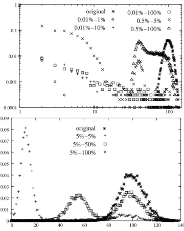
original 0.01%−10% 0.5%−1% 1%−10% 5%−5% 0 2 4 6 8 10 12 14 16 18 20 0.16 0.14 0.12 0.10 0.08 0.06 0.04 0.02 original 0.01%−1% 0.01%−10% 0.01%−100% 1%−5% 0 2 4 6 8 10 12 14 16 18 20 0.18 0.16 0.14 0.12 0.08 0.06 0.04 0.02 0.10
Fig. 10. ER graph: degree distribution. k= 10, N = 104
, USP (top) and ASP (bottom).
Let us first consider ER graphs with low average degree. As shown in Figure 10, if the number of sources is very low then the obtained degree distri-bution is far from the real one. With an USP ex-ploration, the obtained degree distribution converges quite slowly: it is still significantly different from the real one if we take 1% of sources and 10% of
desti-nations. With an ASP exploration, the accuracy is much better: the view is almost perfect even with only0.5% of sources and 20% of destinations.
The case of ER graphs with high average degree (Figure 11) is more interesting: the presence of high degree nodes makes it possible to obtain heteroge-neous degree distributions, well fitted by power laws, with partial USP explorations. This has been stud-ied in previous works [35], [52] to show that the ex-ploration bias may be qualitatively significant. This measurement bias occurs when one considers very few sources and many destinations (Figure 11, top) and the USP exploration. It disappears when one considers a larger number of sources, for instance
0.5% of the whole (Figure 11, bottom), or when one
considers an ASP exploration (Figure 12), even for small numbers of sources and destinations.
Notice also that, in intermediary cases, one may obtain surprising results like the plot for 5% of
sources and50% of destinations in Figure 11, which
has two peaks. As explained in [35], this is due to the fact that in such cases most of the links close to the sources are discovered, whereas the ones close from the destination are not. The rightmost peak then cor-responds to nodes close from the sources (for which we have all their links) while the leftmost one corre-sponds to the nodes close from the destinations (for which we miss almost every link).
These first results concern ER graphs, for which the degree distributions are not power-laws. They show that it is quite difficult to obtain an accurate view of the degree distribution of such graphs, which is improved significantly by the use of many sources and destinations. As already noticed, the use of a low number of sources may even give degree distri-butions qualitatively different from the real ones.
0.01%−100% 0.5%−5% 0.5%−100% original 0.01%−1% 0.01%−10% 0.0001 0.001 0.01 0.1 1 1 10 100 original 5%−5% 5%−50% 5%−100% 0 0 20 40 60 80 100 120 140 0.01 0.02 0.03 0.04 0.05 0.06 0.07 0.08 0.09
Fig. 11. ER graph: degree distribution. k= 100, N = 104
, small number of sources (top log-log scale) and large number of sources (bottom normal scale). USP
If we now consider scale-free graphs, the results are totally different: as one can check in Figures 13 and 14 respectively for MR and DM graphs, both
original 0.5%−100% 0.5%−50% 0.5%−5% 0.01%−100% 0 0 20 40 60 80 100 120 140 0.045 0.040 0.035 0.030 0.025 0.020 0.015 0.010 0.005
Fig. 12. ER graph: degree distribution. k= 100, N = 104
, ASP. original 5%−10% 1%−10% 1%−1% 0.01%−50% 0.01%−10% 0.01%−1% 0.0001 0.001 0.01 0.1 1 1 10 100 1000 original 0.01%−1% 0.01%−10% 0.01%−50% 1%−1% 1%−10% 5%−10% 1e−04 0.001 0.01 0.1 1 1 10 100 1000
Fig. 13. MR graph: degree distribution. α = 2.5, N = 104
, USP (top) and ASP (bottom).
USP and ASP explorations give accurate views of the actual degree distribution6, even for small numbers
of sources and destinations. In the case of MR graphs (the results are similar for AB graphs), the fit is cellent. In the case of DM graphs, the obtained ex-ponent is slightly lower for small numbers of sources
6
The important characteristic of a power-law distribution is its expo-nent α, i.e. the slope of the log-log plot. Here, we divide the number of nodes of a given degree by the total number of nodes N , including the ones which are not discovered during the exploration in concern. This does not change the slope and makes it possible to plot the distributions in a same figure. original 0.01%−5% 0.01%−100% 0.5%−100% 5%−100% 50%−100% 0.0001 0.001 0.01 0.1 1 1 10 100 1 1 0.1 0.01 0.001 0.0001 10 100 original 5%−100% 5%−5% 0.01%−100% 0.01%−10%
Fig. 14. DM graph: degree distribution. N = 104
, USP (top) and ASP (bottom).
but it rapidly converges to the real one.
In conclusion, the behaviors of ER and scale-free graphs are completely different concerning the accu-racy of the obtained degree distributions. Whereas it is quite difficult (especially using an USP ex-ploration) to obtain an accurate estimation for ER graphs, the exponent of the power-law degree dis-tribution of a MR, an AB or a DM graph is correctly measured even with a small number of sources and destinations. Despite the fact that using a very small number of sources and a large number of destinations may give us a wrong idea of the actual degree distri-bution of a graph, we have shown that these cases are pathological. Indeed, as soon as the number of sources grows, this effect disappears.
V. CLUSTERING
The clustering of a graph is computed by divid-ing the number of triangles in the graph by the num-ber of connected triples (see Section I). Just like the average degree depends on the obtained numbers of nodes and links (see Section II), this means that the evaluation of the clustering of a graph we obtain us-ing an exploration depends on how fast we discover
triangles with respect to the speed at which we dis-cover triples: the evaluation of the clustering is accu-rate if we discover a proportion of the total number of triangles similar to the proportion of the total number of triples we discover. We will therefore study how triangles and triples are discovered, together with the clustering itself.
Fig. 15. ER graph: clustering, number of triangles, and number of
triples. k= 10, N = 104
, USP (first row) and ASP (second row).
Fig. 16. Dense ER graph: clustering, number of triangles, and number
of triples. k= 100, N = 104
, USP (first row) and ASP (second row).
Let us first observe what happens for ER graphs. Notice that when the average degree is low, there are almost no triangles in such graphs (and so the cluster-ing is zero). When the average degree grows, so does the clustering. We therefore perform our measure-ments in both cases. As one can check in Figures 15 and 16, there is no real surprise: increasing the num-bers of sources and destinations increases the evalu-ation of the clustering, a consequence of the fact that the speeds at which triangles and triples are discov-ered are quite the same. This is in agreement with the results in the previous section which highlighted the fact that dense sub graph are quite hard to explore.
If we turn to AB and MR graphs (the behaviors of
Fig. 17. AB graph: clustering, number of triangles, and number of
triples. k= 10, N = 104
, USP (first row) and ASP (second row).
the two kinds of graphs are very similar), see Fig-ure 17, we again have a very low clustering but in the USP case it is over-estimated when we consider few sources and destinations. This is a consequence of the fact that we discover much more triangles than triples at the very beginning of the exploration. How-ever, the estimations rapidly becomes accurate, and lower than the initial value. This can be seen in Fig-ure 17: the dark value corresponds to the clustering of the original AB graph, and the only cases where the estimation is wrong are in the lower left corner. The ASP explorations give more accurate results.
Fig. 18. DM graph: clustering, number of triangles, and number of
triples. N= 104
, USP (first row) and ASP (second row).
Let us now observe what happens with a highly clusterized graph, obtained with the DM model. In Figure 18, we can see that the clustering is well eval-uated in all the cases, except if we use much more sources than destinations or conversely (notice that this is currently the case for the explorations of the Internet). Indeed, in these cases, there is a strong difference between the speed at which we discover triangles and triples. When the numbers of sources
and destinations are similar, on the contrary, despite we miss many triangles and triples, the proportions we miss of each are similar. In this case, therefore, the estimation of the clustering is accurate.
In conclusion, we see in this section that when we compute an exploration of a graph with low cluster-ing we may over-estimate the clustercluster-ing. This is due to the fact that the views we obtain are constructed by merging tree-like structures, which makes the tri-angles hard to discover. It seems however that the obtained evaluation of the clustering is quite accurate even for small number of sources and destinations if the underlying graph has a low clustering. On the contrary, if the graph is highly clusterized, we need both a large number of sources and destinations to obtain a good estimation because discovering trian-gles is difficult. This is particularly true when the number of sources or the number of destinations is quite low, which implies that the obtained view is a merging of a few trees and therefore over-estimates the number of triples but contains very few triangles. VI. SOURCES AND DESTINATIONS PLACEMENT
Since not all nodes in the Internet play the same role (there are highly connected nodes whereas most have only a few connections, for instance), one may wonder if it is possible to design placement strate-gies for sources and/or destinations which improve the exploration process. We investigate this idea in this section.
The first well known difference between nodes in the Internet is their degree. We will therefore con-sider the three following simple strategies in which we choose sources and destinations nodes in an or-der depending on their degrees. First we can choose both sources and destinations in increasing order of degrees, therefore we will first conduct traceroutes between low-degree nodes. In another strategy, both sources and destinations can be chosen in decreas-ing order of degree, and finally sources can be cho-sen in increasing order of degree whereas destina-tions are chosen in decreasing order. The other strat-egy (decreasing-increasing) is symmetric. The re-sults should be compared to the ones obtained when we consider sources and destinations chosen at ran-dom, as we always do in the rest of the paper. Notice that many other strategies, based on other statistics, are possible. We only present the simple ones based on the degree, which already gives good insight on
what may happen. For the same reason, we focus on the basic statistics, namely the proportions of nodes and links discovered, and the average degree.
As one may have expected, these strategies make no real difference on ER graphs. Indeed, in these graphs, all the nodes have almost the same degree. Moreover, the quality of the obtained view is good, even for small numbers of sources and destinations (see Figure 2), therefore one cannot expect to im-prove it drastically using any strategy. Likewise, the quality of the exploration of AB graphs is already good even for reasonable numbers of sources and destinations. Therefore, even if placement strategies improve the exploration, the difference is not signif-icant.
Fig. 19. MR graph: number of nodes, number of links, and
aver-age degree. α = 2.5, N = 104
, USP with four strategies (from top to bottom): increasing, decreasing-decreasing, increasing-decreasing, and random. The ASP plots are very similar.
The first case for which the placement strategies are interesting to study is the case of MR graphs, see Figure 19. The obtained results show that sources and destinations placement is definitively relevant: the three strategies give different results, also differ-ent from the random strategy. Moreover, the best strategy seems to be the increasing-increasing one. This comes from the fact that, in scale-free graphs,
it is difficult to discover low degree nodes (see Sec-tion II), whereas they are taken as sources and desti-nations in this strategy (and therefore we ”discover” them quickly). This explains that the increasing-increasing strategy significantly improves the ob-tained view, whereas the decreasing-decreasing strat-egy is inefficient. Notice also that the average de-gree is overestimated in all cases, even with the increasing-increasing strategy. However with this strategy we ensure the discovery of low degree nodes first and the average degree converges faster to its true value.
Fig. 20. DM graph: number of nodes, number of links, and average
degree. N = 104
, USP with four strategies (from top to bottom): increasing-increasing, decreasing-decreasing, increasing-decreasing, and random. The ASP explorations give very similar results.
Finally, let us observe what happens on DM graphs, see Figure 20 for USP explorations (ASP ones give very similar results). In this case, the best strategy depends on one’s aim. If the priority is to discover a large number of nodes using few sources or few destinations, then the best strategy is certainly the increasing-increasing one. This comes from the fact that DM graphs, like MR ones, have a power-law degree distribution and so low-degree nodes are difficult to discover.
However, this strategy gives low performance for
the discovery of links, and gives a highly biased av-erage degree. If these properties are of prime inter-est, one may prefer the increasing-decreasing strat-egy, which also has the advantage of being efficient if the number of sources and the number of destina-tions are more or less equal. This strategy actually has very good performance, in particular if we seek a very accurate view of the graph: it significantly im-prove the number of points above the 0.99-line level. This can be understood as a consequence of the fact that there is a high heterogeneity between sources and destinations.
In conclusion, we see that placement strategies can be used to improve significantly the efficiency of the explorations, but the choice of an appropriate strat-egy is not trivial. Indeed, it depends both on the properties of the underlying graph and on one’s aim. These results are also helpful in understanding the results obtained in previous sections. For instance, they confirm that low degree nodes are difficult to discover, which plays an important role in our ability to map the network.
VII. REAL-WORLD DATA AND EXPERIMENTS Until now, we presented simulations carried out on models of networks and using simple models for tracerouteand the exploration process. We will now make the same kind of experiments on real-world data to evaluate the relevance of these simu-lations.
To achieve this, we will use two the following data sets:
• The first one is a well known map of the
Inter-net called Mercator [27], [28]. It is obtained by using massively traceroute from only one source but with source routing and several other improvements. This map has all the properties we have mentioned: high clustering, power-law degree distribution and low average distance. We will focus on the core of this graph, i.e. the subgraph obtained by iteratively removing the nodes of degree1. Indeed, we have already seen
that the tree-like structures around it are difficult to discover, and our aim is now to identify other properties which may influence the exploration.
• The second data set we will use is the nec
map-ping [44], [42]. It is obtained using282 sources
distributed around the world (public looking-glasses) processingtracerouteprobes from
these sources to282 destinations chosen at
ran-dom in a given set of roughly one thousand IP addresses. The number of sources is therefore huge compared to classical explorations (about ten times higher) whereas the number of desti-nations is quite small. This data set also has an important advantage: we do not only have the map itself but also the actual routes used to con-struct it. As we will see in the following, it will make it possible to deepen some interesting is-sues.
A. Comparison with models
Using these two real-world graphs, we conducted the same experiments as the ones presented above and we compared the results with the ones obtained on a random graph having exactly the same degree distribution (MR model) and on graphs having the same distribution of clique sizes (GL model). The results for the basic statistics are presented in Fig-ure 21 and in FigFig-ure 22 for the core of Mercator and for the nec graphs, respectively. The results concern-ing the clusterconcern-ing are plotted in Figure 23 and 247. The results concerning the average distance and the degree distributions are very similar to the ones ob-served on models, therefore we do not discuss them further.
From Figure 21, Figure 22 and the ones discussed before, we can derive the following interpretations, which are quite similar for the Mercator and the nec graphs, despite the different ways they have been ob-tained:
• the difficulty in exploring these graphs is not
only due to the presence of tree-like structures around the core, since we removed them in the
Mercator graph, and since the nec graph has
al-most no tree-like structure,
• these graphs cannot be viewed as MR graphs
since the exploration of this kind of graphs gives different results, despite the fact we took MR graphs with the very same degree distributions,
• the clustering could be viewed as the main
prop-erty responsible for the low quality of the explo-rations, since the results for the Mercator and
7
The jumps in the grayscale plots for the clustering of the core of the Mercator graph and the nec graph are due to the ones in the plot of the number of triples. Themselves are consequences of the fact that, at this point, we take a very high-degree node as a source with many destinations, which suddenly increases the number of triples (by
d(d − 1) where d is the degree of the node).
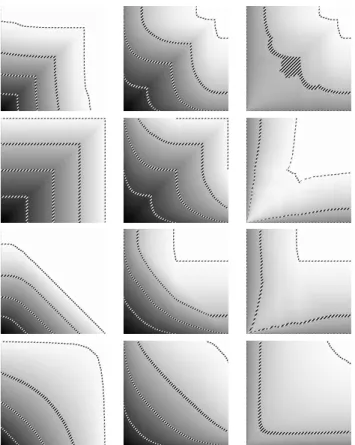
Fig. 21. Number of nodes, number of links, and average degree for
(from top to bottom): the core of the original Mercator graph, a MR graph with exactly the same degree distribution, and GL graph with
the same distribution of cliques sizes.USPexplorations.
Fig. 22. Number of nodes, number of links, and average degree for
(from top to bottom): the nec graph, a MR graph with exactly the same degree distribution, and GL graph with the same distribution of cliques
sizes.USPexplorations.
nec graphs are quite similar to the ones for DM
graphs (Figure 8, first row) and to the ones for GL graphs (Figures 21 and 22, third rows). This last conclusion, however, is not completely sat-isfactory. Indeed, it appears that no model succeed in capturing really well the behavior or Mercator and nec graphs concerning the exploration. This
may indicate that other properties than the degree distribution and the clustering may play an impor-tant role, see for instance the ones proposed in [39]. This can be checked by observing how the cluster-ing is approximated durcluster-ing explorations of our real-world graphs, and exploration of comparable GL graphs, see Figures 23 and 24. From these figures, it seems that the models do not capture all the prop-erties which influence the exploration process, even if the low degree nodes and the clustering have been clearly identified among them.
Fig. 23. Clustering, number of triangles, number of triples for the
core of the original Mercator graph (first row) and a GL graph with
the same distribution of cliques sizes (second row).USPexplorations.
Fig. 24. Clustering, number of triangles, number of triples for the
original nec graph (first row) and a GL graph with the same distribution
of cliques sizes (second row).USPexplorations.
B. Going further
The exact sources and destinations, and the ob-tained routes, used to produce the Mercator graph are not available. Therefore, in this case we cannot plot the grayscale plots where we take the same sources and destinations as in the real exploration, and where we take real routes rather than shortest paths.
This is possible with graphs obtained using more sources and for which we have the information of which routes have been discovered. We have all this information for the nec data set. This makes it possible in this case to compare the grayscale plots obtained using the real traceroute paths to the grayscale plots obtained with shortest paths. This is of prime interest since it allows the evaluation of our hypotheses, like for instance the approximation of real routes with shortest paths.
This lead us to compute grayscale plots where we take the same number of sources and destination as in the original exploration (namely 282 each),
cho-sen at random, and in which we approximate routes with shortest paths, just as before (we used bothUSP and ASP). This gives Figures 25 and 26. Then we compare these plots to the ones obtained when we take the sources and destinations as in the original exploration, and we use the real routes discovered bytraceroute, which gives Figures 27 and 28.
Fig. 25. Number of nodes, number of links, and average degree for the
nec graph using random sources and destinations and shortest-paths.
USP(first row) andASP(second row).
Fig. 26. Clustering, number of triangles and triples for the nec graph
using random sources and destinations and shortest-paths. USP(first
Fig. 27. Number of nodes, number of links, and average degree for
the nec graph using the real routes discovered bytraceroute.
Fig. 28. Clustering, number of triangles and triples for the nec graph
using the real routes discovered bytraceroute.
The plots fit surprisingly well, the results on the real-world data being in general between anUSPand an ASP simulation. This is a very important point, since it gives evidence of the fact that the simulations we conducted throughout the paper rely on reason-able approximations. The results should therefore be considered as relevant, the bias induced by the mod-els of the exploration and of the routes being negli-gible from our qualitative point of view. Let us insist once again, however, on the fact that these results have no meaning from a quantitative point of view.
One may also consider the actual number of nodes one obtains using the maximal number of sources and destinations (here,282), see Table III. When the
sources and destinations are the same as in the origi-nal exploration, and the routes are the real ones, one sees of course all the graph, and the clustering is the real one. With the models, most nodes are discov-ered but approximately one quarter of the links are missed. As already explained, this may be a conse-quence of the presence of links which are between nodes at the same distance from the sources. How-ever, neither an USP nor an ASP exploration can see such links, and Table III shows that here theASP ex-ploration discovers links much better. Therefore, the poor performance of USP is mainly due here to the fact that there exists several (many) shortest paths be-tween sources and destinations. This indicates that repeating the exploration at several dates may help in improving the maps, since one may then discover several shortest paths.
nodes links cc original 1.000 1.000 0.087 random nodes/usp 0.997 0.741 0.0079 random nodes/asp 0.999 0.978 0.012
TABLE III
NUMBER OF NODES,NUMBER OF LINKS AND CLUSTERING DISCOVERED WHEN ALL PATHS HAVE BEEN PROCESSED,FOR ORIGINAL ROUTES AND FOR USP AND ASP EXPLORATIONS WITH
RANDOM SOURCES AND DESTINATIONS.
CONCLUSION AND DISCUSSION
We conducted an extensive set of simulations aimed at evaluating the quality of current maps of the Internet and the relevance of increasing signifi-cantly the number of sources and/or destinations to improve it. To achieve this, we considered the most commonly used models of graphs (namely the ER, the AB, the MR, the DM and the GL ones). Using these simple models has the advantage of making it possible to study separately the influence of various simple statistical properties. We constructed views of these graphs and compared them to the original graphs. We focused on the proportion of the graph discovered (both in terms of nodes and links), the av-erage degree, the avav-erage distance, the degree distri-bution and the clustering, which are among the most relevant statistical properties of complex networks in general, and of the Internet in particular.
We presented in this paper our most significant re-sults. To do so, we introduced the grayscale plots and the level lines, which make it possible to give a synthetic view of a huge amount of information, and to interpret it easily. We also discussed how ex-ploration may be improved by placement strategies for the sources and destinations, and we compared the results on network models to the ones obtained on real-world data. This last point confirmed that the simplifications and assumptions we have made in our simulations do not influence significantly the obtained results.
From these experiments, we derive the following conclusions:
• Two statistical properties of graphs influence
strongly our ability to obtain accurate views of them using traceroute: the presence of many tree-like structures and the high cluster-ing. These two properties act independently and
their effects are combined in the case of the In-ternet.
• It is relevant to use massively distributed
ex-ploration schemes to obtain accurate maps of scale-free clusterized networks like the Internet, in particular if we want to discover most nodes and links, and have an accurate estimation of the clustering. Using more than a few sources should yield much more precise maps.
• On the contrary, the evaluation of the degree
distribution of such a network, as well as its average distance, is achieved with very good precision even for reasonably small number of sources and destinations.
• The details of the exploration scheme (for
in-stance USP versus ASP or the behavior of traceroute) tends to have little importance when the number of sources and destination grows. In the case of the Internet, this means that distributing explorations can be viewed as a way to improve the independence of the results from the exploration scheme and the details of route properties.
• Despite the fact that power-law degree
distribu-tion and high clustering play a role in the ef-ficiency of the explorations of the Internet, it seems that other unidentified properties also in-fluence this efficiency.
• Sources and destinations placement is relevant
for the improvement of the explorations, but the choice of the placement is related to the property one wants to capture. Moreover in real mea-surements, the nodes are indistinguishable be-fore the measurements, therebe-fore such a place-ment is quite challenging and should be modi-fied during the exploration.
Finally, these results make it possible to conclude that we may be confident in the fact that the Internet graph has a very heterogeneous degree distribution, well approximated by a power law, and that the cur-rent evaluation of the exponent of this distribution is quite accurate: current explorations use enough sources to ensure that we do not obtain biased ex-plorations of ER-like graphs, and in the other cases it seems that the estimation of the degree distribution is accurate. Likewise, one might give credit to the available evaluations of the average distance in the Internet. On the contrary, despite the clustering of the Internet is certainly quite high, the estimations
we have should be considered more as qualitative than quantitative.
Much could be done to extend our results. First, one may consider more subtle statistical properties, like the correlations between node degrees, or the correlations between degree and clustering. One may also study more precisely some regimes of special in-terest, like for example the ones currently used (few sources and many destinations), or the one where each source can run traceroute a limited num-ber of times. One should also conduct some experi-ments with more realistic models oftraceroute. Finally, these simulations results may provide some hints and directions for the formal analysis of the quality of Internet maps. Such studies have began [13], [18], but for now only the degree distribution has been studied in specific cases. Much remains to be done in this challenging direction.
Notice also that we only considered here the
router level of the Internet and its exploration
us-ingtraceroute. The same kind of study should be conducted at the Autonomous Systems (AS) level and including other techniques like for example the use of BGP tables. The modeling of such techniques is however a problem in itself.
Finally, let us insist on the fact that most real-world complex networks, like the World Wide Web and Peer to Peer systems, but also social or biologi-cal networks are generally not directly known. Var-ious exploration schemes are used to infer maps of these networks, which may influence the vision we obtain. The metrology of complex networks is there-fore a general scientific challenge, for which the goal is to be able to deduce properties of the real network from the observed ones. The methodology we de-veloped here may be applied to these different cases with benefit.
Acknowledgments. We thank Ramesh Govindan for pro-viding useful data. We also thank Aaron Clauset, Mark Crovella, Benoit Donnet, Timur Friedman and all the Traceroute@Home [55] staff for their helpful comments. This work is supported in part by the ACI S´ecurit´e et Infor-matique project MetroSec [54].
REFERENCES
[1] D. Achlioptas, A. Clauset, D. Kempe, and C. Moore. On the bias of traceroute sampling, or: Why almost every network looks like it has a power law. In ACM Symposium on Theory of Computing
(STOC2005), 2005.
[2] R. Albert and A.-L. Barab´asi. Emergence of scaling in random networks. Science, 286:509–512, 1999.