Comparative Home-Market Advantage:
An Empirical Analysis of British and
American Exports
Rolf Weder University of Basel
Abstract: This paper derives and tests the hypothesis that a country exports relatively more of t h o s e goods for which it has a relatively larger home mar-ket, i.e., a comparative home-market advantage. This prediction is based on a two-country, many-good intraindustry trade model with economies of scale, international transaction costs and differences in expenditure shares and coun-try size. The data from 1970 to 1987 of 26 industries of the manufacturing sector in the United States and the United Kingdom supports this hypothesis. It is also shown that the relationship between home-market size and export structure becomes significantly stronger for industries with high fixed costs. JEL no. F12, F14, F17
Keywords: International trade; home-market advantage; Ricardo; increasing re-turns to scale
1 I n t r o d u c t i o n
This paper has been motivated by t w o rather different strands in the t r a d e literature. F i r s t , t h e r e exists a persistent hypothesis, triggered by the seminal contribution of Linder (1961), that countries export t h o s e products for w h i c ht h e r eis a l a r g e domestic d e m a n d . This "home-market effect" has achieved increasing attention in the t r a d e literature d u r i n g the last few years, in theoretical as well as empirical w o r k J Second,
Remark:I am grateful to an anonymous referee, James Brander, David Green, Richard Harris, John Helliwell, Ronald Jones, Joris Pinkse, Nicolas Schmitt, and participants of seminars at the University of British Columbia, University of Geneva, University of St. Gallen, Simon Fraser University, and the WEA International Conference for helpful comments. Thanks to Peter Lloyd for making me aware of the data. Please address correspondence to Rolf Weder, Department of Economics (WWZ) and Eu-ropainstitut, University of Basel, Gellertstrasse 27, CH-4020 Basel, Switzerland; e-mail: [email protected]
a Conceptual and theoretical contributions include Basevi (1970), Frenkel (1971), Hsu (1972), Krugman (1980), Feenstra (1982), Dinopoulos (1988), Davis (1995,
1998),Tri-there is a straightforward prediction of the pattern of trade made by the Ricardian theory of comparative advantage in the two-country, many-good case. It has b e e n adopted in the pioneering empirical analysis by MacDougall (1951), followed up by others, focusing on the relationship between relative exports and labor costs of the United Kingdom (U.K.) and the United States (U.S.). 2 The main idea of this paper is to con-tribute to the literature on home-market effects by deriving hypotheses from a demand-driven trade m o d e l with monopolistic competition and testing these hypotheses with British and American trade data. Thereby, some analogy to the Ricardian model and how it has b e e n tested will be exploited.
It is well k n o w n that in a framework with constant returns to scale and diminishing returns to each factor of production, a country tends to i m p o r t a good for which its demand is relatively large (Jones 1956). However, suppose that there exists some form of increasing returns to scale. In this case, a large domestic d e m a n d for a certain good tends to p r o m o t e its export rather than its import. For example, firms m a y focus t h e i r R&D efforts on those products for which there exists a large home d e m a n d (Linder 1961; Vernon 1966) which, in a dynamic process, m a y then create comparative advantage and thus lead to exports, as developed further in Bhagwati (1982), Feenstra (1982), and Dinopoulos (1988). The positive relationship also emerges in a static environment if firms face small international transaction costs of exports, as shown by Krugman (1980) in a model o f monopolistic competition. H o m e -market effects m a y also arise in models of oligopolistic competition as s h o w n by, for example, Feenstra e t al. (1998) as well as by H e a d e t al. (2002), who compare different models.
This paper extends the Krugman (1980) approach to the two-country, many-good case and tests whether the predictions of the m o d e l fit the data. The general-equilibrium model assumes that there are two coun-tries that only differ with respect to domestic expenditure shares and c o u n t r y size in a n u m b e r of industries. Hypotheses are then derived
onfetti (2001a), Head et al. (2002). Recent empirical analyses focusing on this issue are Fagerberg (1995), Davis and Weinstein (1996, 1998, 1999), Weder (1996), Feen-stra et al. (1998), Lundb~ick and Torstensson (1998), Head and Ries (2001), Trionfetti (2001b), Briilhart and Trionfetti (2001, 2002a, 2002b).
2 O t h e r analyses of the Ricardian model include Stern (1962) and Balassa (1963). Limitations of this approach are discussed in Bhagwati (1964), Deardorff (1984), and Leamer and Levinsohn (1995).
222 Review of World Economics 2 0 0 3 , Vol. 139 (2)
which focus on the relationship between home-market size and the pattern of trade. First, the m o d e l predicts that countries tend to ex-port relatively more of those products for which the domestic market is relatively large, i.e., where they have a "comparative home-market advantage." Second, the m o d e l suggests that high-economies-of-scale industries conform relatively better to this demand-export hypothesis than other industries. Thus, the degree of scale economies is a n i m p o r t -ant determin-ant of the extent to which d e m a n d affects exports.
The empirical analysis of the relationship between home-market size and the pattern of trade for 26 industries of the U.S. and U.K. manufacturing sector over the period of 1970 to 1987 supports the model's main predictions. In particular, it is f o u n d that there is a pos-itive relationship between relative exports and relative home-market size and that this relationship becomes significantly stronger for in-dustries with high economies of scale. The latter result s e e m s to be especially important. If a n analysis does not (perfectly) control for differences in factor endowment and technologies between countries, a n observed positive relationship between relative home-market size and exports m a y be in line with a traditional trade m o d e l where nei-ther determines the o t h e r one. The findings that the positive rela-tionship is stronger for high-economies-of-scale industries does, how-ever, provide s u p p o r t for the demand-driven m o d e l considered in the paper.
The results relate to a n u m b e r of recent empirical trade papers which consider home-market effects with the purpose of discriminat-ing between the explanatory power of the traditional constant-returns-to-scale and the new increasing-returns-constant-returns-to-scale trade literature. The first empirical papers in this field by Hummels and Levinsohn (1995), Davis and Weinstein (1996, 1998), as well as Lundb~ick and Torstens-son (1998) showed mixed s u p p o r t for home-market effects and the increasing-returns-to-scale literature in explaining volume and pat-tern of trade and production. More recent studies by Feenstra e t al. (1998), Davis and Weinstein (1999), H e a d and Ries (2001), Trionfetti (2001b) as well as Brtilhart and Trionfetti (2002b) have f o u n d sup-port for home-market effects, albeit in rather different settings and with the results needing to be qualified. These studies suggest that in-d u s t r y characteristics s u c h as technology, e n t r y anin-d homogeneity of products are important for the existence and the size of home-market effects. An interesting approach is f o u n d in Brtilhart and Trionfetti
(2001, 2002a), who investigate the effects of home-biased public pro-curement on the pattern of specialization in the European Union. T h e y also find empirical support of home-market effects for this "type of demand. ''3
To show how this paper differs from the literature described above, let m e relate it to the two ideas that are probably most closely linked, i.e., H e a d and Ries (2001) and Brfilhart and Trionfetti (2002b), both of which, however, are b a s e d on different models, empirical methods, trade data and countries. Whereas H e a d and Ries (2001) investigate whether home-market effects become stronger (weaker) - as predicted by the increasing-returns-to-scale (constant-returns-to-scale) industry - d u r i n g a period of substantial trade liberalization between Canada and the U.S., this paper analyzes (among o t h e rthings) whether the relation-ship is stronger in a g r o u p of high-economies-of-scale industries than in a g r o u p of low-economies-of-scale industries. The approach is also dif-ferent from Br/ilhart and Trionfetti (2002b), who estimate home biases for a n u m b e r of industries and countries and then
implicitly
discrimi-nate between constant-returns-to-scale and increasing-returns-to-scale industries by using a gravity model and exploiting the expected rela-tionship between inter-country differences in home biases and patterns of specialization. My paper does not intend to, and cannot, compare the predictive power of the traditional theory with that of the new trade theory, as it only focuses on one example (two countries, a n u m b e r of manufacturing industries with a high share ofintraindustry trade). One contribution of the paper is, however, that it tries to explicitly analyze whether home-market effects become stronger in industries which are characterized by largerfixedcosts and thus a greaterdegree o feconomies of scale.The remainder of the paper is organized as follows. Section 2 d e -scribes the m o d e l of comparative home-market advantage and the hy-potheses following from it. The description of the data c a n be f o u n d in Section 3. The empirical analysis and the interpretation of the results are carried out in Section 4. Section 5 concludes.
3 N o t e also Fagerberg (1995), who investigates the international competitiveness of
vertically related industries, as measured by an index of revealed comparative advan-tage (RCA). He finds some positive relationship between user and supplier industries' RCA for a n u m b e r of industries and OECD countries which, again, can be interpreted as support for a demand-related explanation of the pattern o f trade.
224 Review of World Economics 2003, Vol. 139 (2)
2 T h e M o d e l a n d Its Hypotheses
Imagine a world w i t h two countries, home a n d foreign, that only differ w i t h respect to t h e i r home-market size f o r different goods. In particular, it is assumed that consumers in the home and foreign c o u n t r y spend different shares o f t h e i r income (s a n d s*) o n the available goods a n d that t h e two countries m a y also have a different p o p u l a t i o n size (L and L*).4 Each good is c o m p o s e d o f m a n y varieties w h i c h are produced at de-creasing average costs. T h e r e is only o n e factor o f production, l a b o r , w h i c h is perfectly mobile within each country. Finally, t h e r e are small
international transaction costs (t > 1) o f the iceberg type, w h i c h can be
interpreted so as to i n c l u d e any i n c r e m e n t a l variable costs associated
w i t h the supply o f goods to the o t h e r m a r k e t .
The relationship between home-market size and p a t t e r n o f t r a d e is discussed in Section 2.1 f o r the two-good case w h o s e derivation can be f o u n d in W e d e r (1995) as a n extension o f K r u g m a n (1980). In Sec-tion 2.2, the m o d e l is e x p a n d e d to the m a n y - g o o d case a n d comparative statics results are derived. Section 2.3 establishes the empirical h y p o -theses.
2.1 T w o - G o o d C a s e
T h e representative consumer's preferences in the home (foreign) c o u n t r y are described by a C o b b - D o u g l a s u t i l i t y function, U ( U * ) , w i t h a con-stant share o f i n c o m e , si(s*), spent o n goods 1 and 2:
2,
* * * = 1. (1)
w h e r e s i , si > 0 ; s l + s z = l ; s l + s 2
U* *sT ,s~
= C 1 C2 ,
Each c o n s u m p t i o n aggregate Ci(C*) o f home (foreign) consumers is c o m p o s e d o f m a n y varieties w h i c h e n t e r symmetrically a CES subutility function, where ca (c~) are the quantities o f consumption o f t h e j t h variety o f good i, p r o d u c e d in the home (foreign) country:
F/i ~/~
, ~-, C.O
C i , Ci = j=l• co + j=zL-i=~J ' where 0 < 0 < 1. (2)
4 For example, consumers in the U.K. may spend a larger share of their expenditures on small cars than the consumers in the U.S. However, given the larger number of consumers in the U.S.,the home market for small cars is likely to be absolutely smaller in the U.K. than in the U.S.
The endogenous n u m b e r of varieties produced in the home (foreign) c o u n t r yis denoted by n i ( n ~ ) . The constant elasticity of substitution and price elasticity of demand is equal to o" = 1/(1 - 0). The production of each variety is subject to decreasing average costs, which is represented b y t h e cost function in terms of labor, lij = a + bxij (a, b > 0), with fixed costs, a, and constant marginal costs, b, where lij describes the a m o u n t of labor u s e d in the production of x u n i t s of o u t p u t of the jth variety of the composite good i. The technology is identical in both countries and in all groups of goods.
In the open-economy equilibrium, home and foreign consumers maximize their utility by taking into account the different prices of home and foreign produced varieties of each good. Simultaneously, firms maximize profits in a setting of monopolistic competition by following the usual markup-pricing rule. E n t r yensures that, in equilibrium, profits are driven down to zero. The profit-maximizing o u t p u t (xij) of all firms in both groups of goods and both countries is identical and independent of market size, which is due to the a s s u m e d utility function:
a ( O )
a
Xij = X/j = ~ = g(O" - - 1 3 . ( 3 )
The relationship between the two countries' home-market size for the two groups of goods and the pattern of trade is established by deriving the general equilibrium, i.e., the relative n u m b e rofvarieties produced by the two countries in free trade. The following e x o g e n o u s "home-market coefficients" c a n then be introduced which capture the home-market size of each g r o u p of products: s l L = M 1 ,s 2 L = M 2 ,s~L* =- MI,S2L* * * = M~.* If the foreign country has a m u c h larger population than the home country, it is likely to have a n absolutely larger home market in both groups of goods, i.e., M~ > M1 and M~ > M2.
It c a n be shown that, in spite of its absolute home-market disadvan-tage in both goods, the home country is a (net) exporter of that g r o u p of good where it has a relatively larger home market, i.e., where it has a c o m p a r a t i v e h o m e - m a r k e t a d v a n t a g e ( W e d e r 1995: 351).5 Thus, the home country's balance of trade for good 1 is positive if and only if the
5 T h e notion " ( n e t ) exports" refers t o the point that there may or may n o t exist two-way trade in a good. T h e lower transport costs and the bigger relative differences in home-market size are, the more likely a complete specialization is.
2 2 6 Review of World Economics 2 0 0 3 , Vol. 139 (2)
following condition holds:
M1 M~ (4)
M2 M~"
The intuition is as follows. Suppose the two countries are identical in size (L = L*) - as a s s u m e d in Krugman (1980) - and that the home country's residents s p e n d a larger p o r t i o n of their income on good 1 (Sl > s~). In this case, the home country's firms producing g r o u p 1 varieties have a transaction cost advantage compared to their foreign competitors because of the absolutely larger home market in this g r o u p of products. Thus, relatively more firms in the home c o u n t r y enter g r o u p 1. Exports are boosted by a n increase in the n u m b e r of varieties of
g o o d 1 .6 The home c o u n t r y is a (net) exporter of good 1 and the foreign c o u n t r y a (net) exporter of good 2.
Now suppose the home c o u n t r y is m u c h smaller than the foreign country. Thus, the foreign country is likely to have a n absolutely larger home market in both groups of products. This implies that the foreign c o u n t r y faces a b o o s t in its exports because of its absolute home-market advantage in both goods. However, this situation w o u l d lead to a trade surplus for the foreign country and a l a b o r shortage in its labor mar-ket. The endogenous relative wage therefore compensates for the greater "competitiveness" of the foreign country's firms. The foreign country thus enjoys a higher wage rate in equilibrium (w* > w). This process establishes the analogy to the Ricardian trade model. Countries tend to be (net) exporters of that g r o u p of goods in w h i c h they have a compar-ative home-market advantage. Absolute advantages are reflected in the equilibrium wage rate.7
2.2 Many-Good Case and Comparative Statics
Let m e now establish the general equilibrium for the many-good case and ' derive some comparative statics. An increase in the n u m b e r of composite goods from 2 to G expands the utility function in (1) in a straightforward
6 W e may denote this as a "magnification effect" as suggested by Trionfetti (2001b: 405) in this type of model.
7 N o t e t h a t , like in the Ricardian model, absolute and comparative advantage is de-fined in terms of an exogenous variable (expenditure share times population) and does n o t include the wage rate.
manner, where
shares of good i, respectively:
G
v = F l q ' ,
i=1 GC~t
U* = I ~ , , i=1si and s~ are home and foreign consumers' expenditure
G G
where ~ Si = ~ S~ = 1. ( 5 )
i=1 i = l
It c a n be s h o w n that the relationship betweencomparative home-market advantage and pattern of trade, described in Section 2.1, also h o l d s in the many-good case. First, the equilibrium relative wage rate,w / w * ,is determined by using the balanced trade condition and remains a positive function of the relative country size, L / L * , and the parameters of the model (see A 1 - A 3 in the Appendix):
L ( w / w * ) ~ - t 1-°
L--7 = ( w / w . ) l _~ _ ( w / w , ) t l _ . (6) Second, as wagesadjust for the difference in country size according to (6), the home and foreign expenditure shares and thus relative home-market sizes remain decisive to explain the pattern of trade. By calculating ex-p o r t s of the home ( X i ) and foreign country (X~) in the open-economy equilibrium for good i, the following relationship between relative ex-p o r t s and relative home-market coefficients c a n be f o u n d (see A 3 - A 5 in the Appendix):
Xi ( M i / M i * ) [ 1 - - q ( w / w * ) ] + [ q q * ( w * / w ) - - q] Xi* ( L / L * ) [ 1 - q * ( w * / w ) ] + ( M i / M * ) [ q q * - - q ( w / w * ) ] '
(7)
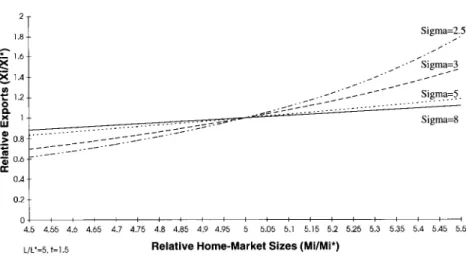
where q = ( w / w * ) ~ - l t1-~ and q* = ( w * / w ) ~ - l t 1-°. Equations (6) and (7) determine the general equilibrium of the model. We are now interested in two questions - first, how relative exports depend on relative home-market size and, second, how this relationship is affected by a change in the degree of economies of scale. As the relationship depictedby (7) is quite complex, it will first be simulated and then be solved for one special case. The simulated example in Figure 1 assumes that international transaction costs are one-third of average costs (t = 1.5), the home c o u n t r y is five times as big as the foreign country ( L / L *= 5), and the relative wage is determined by (6).228 Review of World Economics 2003, Vol. 139 (2)
Figure 1: Relative Exports and Relative Home-Market Sizes (simulation)
2 1.8 Sigma=2.5 1.6 ~- j / " ' t " ~..~ Sigma93 X~-- 1.4 ~ " ~ ~ ~ [. . . Sigmas5.. 1.2 ~ - ' ~ 0 . . . . ~.-.::_--x I Sigma=8 nl 0.8 ..--. 0.6 0.4 0.2 4.5 4.55 4 6 4.65 L/L*=5, t= 1,5 4'.7 4.75' 4'.8 4.85. 4.9 4,95. . 5. 5.05. 5.1. 5 15: 5'~ 525' 5 3i 5.35' 5 4i 5.45' 5.5' Relative H o m e - M a r k e tS i z e s (Mi/Mi*)
First, note from Figure 1 that there is a positive relationship between relative exports (Xi/X*) and relative home-market size ( M i / M * ) for any given o-. This means that, for a given equilibrium wage rate, the home country's exports are relatively higher in those industries where domestic expenditure shares are relatively greater. The two countries' exports are identical in that industry where expenditure shares in the two countries happen to be identical, i.e., where the home country's home market is just five times as big as the foreign country's ( M i / M * = L/L* = 5). This is possible because the home country's larger popula-tion size (L > L*) is reflected in a higher wage rate (w > w*), which makes sure that the relative home-market size determines the pattern of trade.
Figure 1 thus implies t h a t , for given parameters (or, t), we c a n order and renumber all goods in a chain of decreasing relative home-market size. We calculate the ratio of the two countries' home-market size for each good i and take into account that M i / M * equals L/L* for that good of which the relative expenditure share (si/s*) happens to be equal to one. Thus,
M1 M2 L Mi MG
- - > - - > . . . > - - > - - . > - - > . . . > - - . ( 8 )
M~ M~ L* M~ M~
The home country tends to export relatively more of those g o o d s with a low index, the foreign c o u n t r y relatively more of those with a high
index. The relative c o u n t r y size
(L/L*)
determines where this "chain of comparative home-market advantage" is broken and, thus, of which goods the home country exports relatively more than the foreign coun-try.8 There m a y exist complete specialization with respect to some goods (more likely for those a t the two ends of the chain), whereas o t h e r goods m a y be produced by both countries.Second, Figure 1 reveals that the positive relationship between rela-tive exports
(Xi/X~[)
and relative home-market size(Mi/M*)
becomes stronger for smaller values of a as indicated by the steeper dotted lines. A smaller elasticity of substitution implies a higher mark-up p e r firm, which positively affects producer prices and the relative cost advantage of firms with a larger home market. This tends to increase home-market effects. Note that in the m o d e l a change in a affects relative exports not only directly t h r o u g h (7), but also indirectly t h r o u g h a change in the relative wage rate in (6). The total effect is captured by Figure 1 for different values of a.9In interpreting this result, it is important to note Krugman's (1980: 957) description of a as a n inverse "index of the importance of scale economies." The p o i n t is that a lower elasticity of substitution causes a lower o u t p u t p e r firm in equilibrium, as c a n be seen from (3). As fixed costs are spread over f e w e r units, average costs become m u c h higher than marginal costs. The ratio of total variable costs,
bxij,
over fixed costs, a , thus decreases with smaller a in (3). A lower a can therefore be interpreted as a situation that is consistent with relatively high fixedcosts and, therefore, a greater degree of economies of scale in equilibrium.As emphasized by a referee, a change in fixed costs, a , does not affect the magnitude of home-market effects in this particular model because of the constant elasticity of substitution. An increase in fixed costs w o u l d simply shift out the average cost curve and make firms produce a larger quantity a t the same price a s before (equation (3)). In o t h e r more complex models, however, a n increase in fixed costs m a y influence the elasticity of substitution, and thus prices, which in turn w o u l d magnify home-market effects. For example, in a monopolistic competition m o d e l with linear d e m a n d and a continuum of goods - the
8 Equation (8) demonstratesthe analogyto the Ricardian model with its "chain of de-creasing relative labor costs;" see, e.g., Jones and Neary (1984: 12).
230 Review o f World Economics 2 0 0 3 , Vol. 1 3 9 (2)
one introduced by Ottaviano e t al. (2002) -, a change in fixedcosts w o u l d increase home-market effects, as also shown by H e a d e t al. (2002). l°
Note that the two results discussed above c a n be derived as a n explicit solution of (7) for the special case where countries are equal in size (L = L*). In this case, wages are identical (w = w*) in equilibrium as s h o w n by (6), which greatly simplifies (7) to
X i (lVli/M*) - t 1-~
X ~ = 1 - ( M i / M ~ ) t 1-~" (9)
Differentiation of (9) with respect to relative home-market size, M i / M ~ , yields
3 ( X f f X * ) 1 - - t 2-2~
- - > 0 , ( 1 0 )
3 ( M i / M * ) [1 - ( M i / M * ) t l - o ] 2
since t and cr are greater than 1. This confirms that relative exports are increasing in relative home-market size. Differentiation of (9) with respect to the index of economies of scale, o-, yields
O(Xi/X. ) _ _ t 1-o In (t) [1- - ( M / / M * )2] (11)
O~ [1 -- ( M i / M * ) t t - ~ ]2
This first derivative is negative (positive) if M i / M * is greater (smaller) than 1 and it is equal to zero if Mi/Mi* is equal to one. This means that relative exports of the home country increase with a greater degree of economies of scale (i.e., smaller or) in those industries where the home country's market is larger than abroad. Relative exports decrease for domestic industries with a smaller home market and they do not change for industries for which the home and foreign country's home market is identical. These results are in line with the simulation in Figure 1. The difference is that, in this special case, the functional relationship between relative exports and home-market size goes t h r o u g h and pivots a t the p o i n t where X i / X * = 1 and M i / M * = si/s* = 1.
2.3 Empirical Hypotheses
The m o d e l and its comparative statics thus i m p l y two hypotheses for the two-country, many-good case: (1) a c o u n t r y exports relatively more of
10 Another approach w o u l d be Krugman (1979) with an endogenous elasticity of sub-stitution.
those goods for w h i c h its home market is relativelylarger, (2) the posi-tive relationship between relaposi-tive home-market size and relaposi-tive exports becomes stronger if production is characterized bylarge scale economies. As the paper has b e e n motivated by the Ricardian model and its empirical analyses, the investigation of these two hypotheses will be b a s e d on exports of the U.S. and the U.K. to t h i r d countries for a n u m b e r of industries, i. Thereby, a linear relationship between relative exports
(E~ s ~ElvK)
and relative home-market size(M~ s/MiuK)
is a s s u m e dwhich c a n simply be estimated by the ordinary least squares estimator
(OLS):
M?S.
- - t~0 + t~I ~ i u . K . -~- Ei. ( 1 2 )
E~./c.
Note that the model predicts
apositive
slope coefficientas U.S. exports are expected to be relatively higher in those industries where the U.S. home market is relatively larger. Also recall that, in the model,Mi
has b e e n defined as the country size (L) multiplied by the expenditure share(si).
Thus, M/reflects the
real
absolute home-market size, which could be interpreted as the n u m b e rof"people equivalents" who buy good i.11 This variable will not be available in the data. If, however, we multiplyMi
by the equilibrium wage rate, w, we arrive a t a
monetary
variable of market size ( L s i w ) , which reflects the income or total expenditures of the economy spent on good i. Alternatively, we could reduceMi
to the expenditure share of goodi, si,
by dividingMi
t h r o u g h the population size, L, as discussed when establishing (4). In the empirical part, we will apply the first option, because it keeps the possible distinction between absolute and comparative home-market advantage introduced in Sections 2.1. and 2.2.12 Also note the three following considerations when stepping from the theoretical model to its empirical analysis.11 N o t e t h a t , in the model, each consumer buys a little bit o f all varieties o f each good.
12 T h e difference between defining Mi in terms of expenditure share (si)o r in terms o f the value o f home-market size (Lsiw) is basically that the explanatory variable is multiplied b y a constant for all industries (e.g., by the relative equilibrium wage rate,
w g S ' / w UK, in order t o obtain the value o f relative home-market size). As long as we d o a cross-section analysis at a certain point in t i m e with a given relative wage rate, the quality o f the results will be the same for both cases. If different periods (panel data) with, for example, a changing relative wage r a t e over t i m e are included, the re-sults of the two options could, in principle, differ. W e will c o m e back t o this point in the empirical p a r t .
232 Review of World Economics 2 0 0 3 , Vol. 139 (2)
First, it is a s s u m e d that there is a linear relationship between relative exports and relative home-market size. As c a n be seen from (7), the m o d e l does not predict this linearity, in general. Note, however, that it is not the m o d e l with its precise functional form which will be analyzed below. The main interest of the empiricalanalysis belongs to the model's comparative statics as simulated in Figure 1 and explicitly derived in (10) and (11) for a special case. To w h i c hextent relative exports increase with rising relative home-market size, i.e., the sign of the second derivative, will highly depend on the precise specification of the model. The im-p o r t a n t im-prediction to be tested is that the relationshiim-p is im-positive and that it becomes steeper with a greater degree of economies of scale.
Second, the model is a b o u t trade in f i n a lgoods - which is the case for a large body of international t r a d e t h e o r y - whereas the data includes t r a d e of products a t various stages of production. Note, however, that the m o d e l c o u l d be t h o u g h t of as to describe a relationship between exports and home-market size of intermediate products by interpreting the utility and subutility functions as production functions where a n endogenously determined n u m b e r of intermediate products enters the production of final goods (see Ethier 1982:391).
Third, the empirical analysis concentrates on relative exports of the two countries to third markets. The reasons are analogous to the ones b r o u g h t forward in the empiricalanalyses of the Ricardian trade model.~3 Taking bilateral trade flowsw o u l db r i n g the disadvantage that these flows are typically m u c h smaller and more volatile than third-country exports and that they are usually distorted by asymmetric trade protection by the two investigated countries.14 Mso note that, similarly to the Ricardian model, our "home-market model" is principally in line with s u c h a n empirical investigation, because relative cost advantages c r e a t e d by dif-ferences in the home-market size will also carry over to the two countries' competitive position in t h i r d markets. Thus, we compare the relative ex-port performance of the two countries in a n u m b e r of industries in t h i r d
13 See MacDougall (1951), Stern (1962) and Balassa (1963), who all focus their ana-lyses o f the Ricardian model o n exports t o third countries despite the fact that the Ri-cardian model is discussed in a two-country setting. Deardorff ( 1 9 8 4 : 477) supports this approach even though it has been criticized by Bhagwati (1964).
14 N o t e that in a multilateral trade system a third-country's import barrier is likely t o affect the two countries' exports symmetrically (most-favored-nation principle), whereas each of the two countries' trade barriers might very well differ and thus dis-tort bilateral t r a d e flows.
markets and investigate whether this performance is positively related to the exporting countries' relative home-market size. The relative third-market access for different industries is, therefore, a s s u m e d to be equal for both exporting countries.
3 Data Description
The empirical analysis focuses on the complete ISIC groups 38 (manu-factures offabricatedmetal products, machinery and equipment) and 39 (other manufacturing industries) of the manufacturing sector, is T h e y include 26 industries on the 4-digit ISIC level, representing 60 percent of total U.S. and 50 percent of British exports of manufactured goods (see Table 1). These two groups seem to be in line with the model's main assumptions, as the industries are not resource-based and, a t the same time, are characterized by a high share of intraindustry trade as m e a s u r e d by the Grubel-Lloyd index.16 The figures are from the Inter-national Economic Data Bank (IEDB) and include yearly data for the period 1970-1987 in U.S. dollars.17
Note that the figures in Table 1 are yearly averages of the two c o u n -tries' third-market exports
(Ei)
and home-market sizes(Mi).
H o m e -market sizes are calculated by taking production plus imports m i n u s exports p e r industry. This so-called "apparent consumption" corres-p o n d s to actual domestic consumcorres-ption and thus home-market size corres-p e r industry if there are no changes in inventories. This suggests to focus the analysis on long periods in order to eliminate changes in inventories. The figures s h o w n in Table 1 are one example of tong-term averages15 N o t e that two industries within class 3 8 have been eliminated because of obvious data errors: ISIC 3801 (negative consumption over the whole period of investigation) and ISIC 3 8 4 9 (not reported by the U.S. after 1987 and showing a huge and u n u s u a l deviation from OECD trade data (OECD 1993) b y a factor of 2 5 t o 90).
16 Other ISIC groups include many industries whose production is heavily dependent o n resource endowments (e.g., dairy products in g r o u p 3 1 , basic industrial chemicals in g r o u p 3 5 or iron and steel basic industries in group 37). This is confirmed by the Grubel-Lloyd index of intraindustry trade ( G r u b e l and Lloyd 1975), which turns out t o be highest for 3 8 and 3 9 in both countries relative t o all other ISIC groups. 17 IEDB is at the Australian National University (Canberra). T h e n u m b e r o f 4-digit industries is larger than the one provided by the OECD in its "Industrial Structure Statistics," and third-country exports can be derived. Trade and production data are matched o n a 4-digit ISIC level b a s e d o n UN COMTRADE (trade) and OECD COM-TAP (production) data.
234
Table1:
R e v i e w o f W o r l d Economics2 0 0 3 , Vol. 139 (2)
U.S. and U.K.Exports to Third Countries and Home-Market Size,
1970-1987 (yearly average;1.000 U.S.dollars)
Exports Home market
Industries (ISIC 38 and 39) U.S. U.K. U.S. U.K.
3811-CUTLERY, HAND TOOLS 927,481 365,199
3812-FURNITURES, FIXTURES 113,286 51,721
3813-STRUCTURAL METALP R O D U C T S 1 , 4 6 7 , 1 0 5 922,842
3819-FABR MET PRD EXC MACH EQP NEC 1,649,474 1,181,604
3821-ENGINES, TURBINES 412,878 206,196
3822-AGRIC MACHINERY AND EQUIP 936,043 357,395
3823-METAL & WOODWORKING EQUIP 1 , 2 7 0 , 9 2 6 586,671
3824-SPEC IND MACH & EQP EX 3823 6,170,871 2,753,173
3825-OFF, COMPUTG,ACCOUNTG MACH 6,302,517 1,971,466
3829-MACH,EQUIP EX ELECT NEC 6,487,846 2,717,159
3831-ELEC IND MACH & APPARATUS 998,256 475,092
3832-RADIO, TELE, COMM EQP,A P P A R 7 , 9 6 9 , 0 0 5 2,584,673
3833-ELEC APPLNCS & HOUSEWARES 146,014 95,168
3839-ELEC APPAR & SUPPLIES NEC 1,350,795 733,823
3841-SHIPBUILDING & REPAIRING 1,221,357 760,781
3842-RAILROAD EQUIPMENT 414,094 118,003
3843-MOTOR VEHICLES 13,327,179 4,309,322
3844-MOTOR CYCLES & BICYCLES 81,327 93,103
3845-AIRCRAFT 9,747,007 2,556,737
3851-PROF, SCIEN, MSRG, CNTRL EQU 3 , 7 3 3 , 0 3 4 1,481,025 3852-PROF, SC, MSRG, CONT EQU NEC 1 , 1 0 1 , 0 0 5 531,013
3853-WATCHES & CLOCKS 68,394 61,748
3901-JEWELRY & RELATED ARTICLES 447,391 1,374,672
3902-MUSICAL INSTRUMENTS 102,639 35,053
3903-SPORTING & ATHLETIC GOODS 63,007 22,523
3909-MANUF INDUSTRIES NEC 332,482 263,608
Percent o f Total Manufacturing(3000) 60% 50%
9,956,154 800,666 6,364,778 627,638 22,838,990 4,119,450 53,661,566 8,471,248 4,660,475 834,683 10,804,754 1,893,177 16,112,689 1,248,276 22,203,140 4,276,552 24,365,495 3,040,063 56,157,942 10,060,403 22,306,461 3,736,831 66,887,063 8,585,906 4,146,195 1,028,046 18,799,187 3,271,421 11,377,280 1,547,750 3,548,156 307,701 141,303,053 14,054,101 2,229,602 316,603 33,267,196 2,619,614 16,691,501 2,675,848 9,812,964 787,260 1,988,996 461,226 4,647,076 782,304 924,115 127,134 2,946,172 287,498 11,567,355 2,040,870
Source: B a s e d o n data f r o m IEDB (Australian N a t i o n a l University).
(18-year averages). Shorter time periods will also b e considered in t h e empirical analyses. Also note that t h e s e figures include intermediate a n d final products as mentioned above.
4 Empirical Analysis
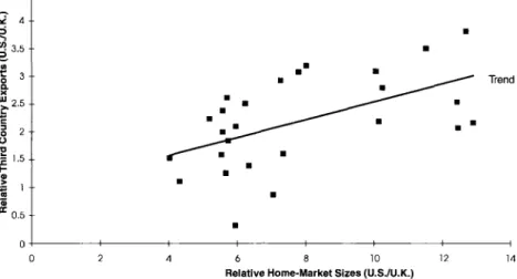
T h e relationship between t h e ratio of U.S. to U.K. home-market size a n d t h e ratio of U.S. to U.K. exports to third countries is illustrated b y Figure 2 for t h e 26 industries described in Table 1. Note that Figure 2 is based o n t h e longest period, i.e., 19701987 averages of exports a n d h o m e -market size. T h e picture suggests that there exists a positive relationship between relative exports a n d relative home-market size. T h u s , t h e larger
the U.S. relative to the U.K. home market, the larger U.S. relative to U.K. third-country exports are. Also note that the home-market size is absolutely larger in the U.S. for all industries (the ratio starts a t 4) because of the m u c h larger country size of the United States. Exports of the U.S., however, are generally not as m u c h larger and e v e n smaller for a few industries. This, again, is in line with the m o d e l which proposes that comparative and not absolute home-market advantages determine the pattern of trade. So, in a r o u g h w a y a t least, Figure 2 provides some
Figure 2: Relative Exports and Home-Market Sizes o fthe U.S. and the U.K. (average o f 1970-1987) 4.5 ~. 3 . 5 w "~ 3 & x ~2.5 ~ 2 0 2 ~. ] . 5 Im ~ 1 -g 0.5 • •m T r e n d I I I I I I I 2 4 6 8 10 12 14 R e l a t i v e H o m e - M a r k e t S i z e s (U.S./U.K.)
s u p p o r t of the positive relationship between relative home-market size and relative exports. This first hypothesis will be tested more carefully in Section 4.1, whereas Section 4.2 is devoted to the second hypothesis regarding the different behavior of h i g h - and low-economies-of-scale industries.
4.1 Exports and Home-Market Size
The estimation of the first hypothesis by OLS confirms the picture given by Figure 2. Taking averages of relative exports and relative home-market sizes over the whole time period (1970-1987), the regression provides
236 Review of World Economics 2003, Vol. 139 (2) the following result:
E u's" M v's" - 2
-- 0.93* + 0 . 1 6 " * - - (R = 0.26). (13)
E U.K. (0.42) (0.05) M U.K. '
The coefficient,/31 = 0.16, has the expected sign a n d is significant a t the 1 p e r c e n t level w i t h a t - v a l u e o f 3.16. T h u s , the null hypothesis,/31 _< 0, is rejected. This result supports the prediction o f the model. In o r d e r to investigate w h e t h e r this relationship is relatively constant a n d t o exploit the full i n f o r m a t i o n available f r o m the data set, a n u m b e r o f regressions have been p e r f o r m e d f o r different subperiods and p o o l e d data. Table 2 r e p o r t s the results.
F o r the n o n p o o l e d estimations, it is f o u n d that the slope coefficient has the expected positive sign in all subperiods, i.e., in the different 9-, 6-, a n d 3 - y e a r averages. T h e null hypothesis that the coefficient is e q u a l t o o r s m a l l e r than zero is rejected in all cases (8 times o n the 1 p e r c e n t and 4 times o n the 5 percent significance level). 18 In o r d e r to get b e t t e r estimates o f the coefficients, one m a y w a n t to exploit the full informa-tion f r o m the data set by p o o l i n g the different periods, i.e., each o f the 9-, 6-, 3-, a n d 1-year averages. OLS estimations reveal that the slope coefficient is positive a n d h i g h l y significant in all regressions (see the
l o w e r part o f Table 2).19 An examination o f first-order autocorrelation
between a n industry's residuals over time shows, however, that the es-t i m a es-t e d aues-tocorrelaes-tion coefficienes-ts (p) are significanes-tly differenes-t f r o m zero implying that the t-values m a y b e overestimated.
This is t a k e n into account b y the generalized least squares estimator (GLS), i.e., the application o f OLS t o the data t r a n s f o r m e d by a
"quasi-first-difference t r a n s f o r m a t i o n " [GLS (Auto)]. 2° In addition, Table 2
18 As ratios are taken for the dependent and independent variable, we would not ex-pect error terms to be correlated between industries. A Goldfeld-Quandt test as well as the calculation of the White estimator showed no evidence of heteroskedasticity.
19 If we replace absolute home-market sizes (Mi) by the expenditures shares (si),the
results remain qualitatively unchanged. All coefficients in the pooled regressions are
significantly different from zero. We thus limit the furtherempiricalanalysis toM i as
proposed and discussed in the theoretical part.
2o Assume relative exports of industry i and time period t are denoted byEt. The
"quasi-first-order transformation" implies that for all time periods except the first one
we calculate new values ofE(E~)whereE't = E t -- pEt-1. For the firstperiod, E~ =
( 1 - p2)l/2E1 is applied in order to keep as many observations as possible
(Prais-Winston transformation). This standard procedure is also applied to the independent variable (relative home-market size).
T a b l e 2 : Results o f OLS/GLS-Estimations for 26 Industries, Different Periods and Pooled Data
Estimation p e r i o d s S l o p e t-value o f]31 R2 No. o f
coefficient ( a d j . ) obser-(fll) v a t i o n s N o n - p o o l e d estimations ( O L S ) 7 0 - 8 7 0.16"* 3.16 0.26 2 6 7 0 - 7 8 0.26** 4.01 0.38 2 6 7 9 - 8 7 0.13"* 2.66 0.20 2 6 7 0 - 7 5 0.28** 4.30 0.41 2 6 7 6 - 8 1 0.14"* 2.50 0.17 2 6 8 2 - 8 7 0 . 1 2 " 2.47 0.17 2 6 7 0 - 7 2 0.20** 3.18 0.27 2 6 7 3 - 7 5 0.34** 5.01 0.49 2 6 7 6 - 7 8 0.21"* 3.36 0.29 2 6 7 9 - 8 1 0 . 1 1 " 1.88 0.09 2 6 8 2 - 8 4 0 . 1 3 " 2.43 0.16 2 6 8 5 - 8 7 0 . 1 2 " 2.16 0.14 2 6 P o o l e d e s t i m a t i o n s (OLS/GLS) 9-year averages p = 0.47 - OLS 0.20** 4.82 0.30 52 - GLS (Auto) 0.24** 5.59 0.37 52 - GLS (Auto, H e t ) 0.24** 3.77 0.37 52 6-year averages p = 0.54 - OLS 0.19"* 5.68 0.29 78 - GLS (Auto) 0.22** 6.52 0.35 78 - GLS (Auto, H e t ) 0.22** 3.63 0.35 78 3-year averages p = 0.72 - OLS 0.19"* 7.68 0.27 156 - GLS (Auto) 0.18"* 7.09 0.24 156 - GLS (Auto, H e t ) 0.18"* 5.05 0.24 156 1-year averages p = 0.85 - OLS 0.18"* 12.81 0.26 468 - GLS (Auto) 0.15"* 9.91 0.17 468 - GLS (Auto, H e t ) 0.15"* 6.26 0.17 468
** significant at t h e 1 percent level. - * significant at t h e 5 percent level. - GLS (Auto) = OLS i n transformed data, corrected for first-order a u t o c o r r e l a t i o n . - GLS (Auto, H e t ) = OLS i n transformed data, corrected for first-order a u t o c o r r e l a t i o n and a p p l y i n g t h e W h i t e e s t i m a t o r for an u n k n o w n form o f heteroskedasticity.
2 3 8 Review of World Economics 2 0 0 3 , Vol. 1 3 9 (2)
also reports the White estimator on the transformed data [GLS (Auto, Het) ], which corrects for a n u n k n o w n form ofheteroskedasticity. Table 2 shows that the slope coefficient remains significantly different from and greater than zero in all corrected pooled regressions on the 1 percent significance level.21 Thus, we conclude that there is a highly significant positive relationship between relative exports and relative home-market size for the nonpooled and pooled regressions.
RESULT 1: There is strong support of the first hypothesis that exports are relatively higher in those industries where the home market is relatively larger.
4.2 Scale Economies
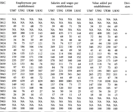
The question is whether greater increasing returns do cause greater home-market effects, as suggestedby the model. The analysis of this sec-ond hypothesis requires to select industries with high economies of scale and to test whether the slope coefficient of the high-economies-of-scale industries is significantly greater than the one of the other industries. Given the restrictions from the data which has to provide any informa-tion for the s a m e industry classificainforma-tion u s e d in the trade and producinforma-tion data, I use higher average firm size as a proxy for greater fixed costs and thus larger economies of scale a m o n g the 26 industries. B a s e d on the available data, the ratio of (i) employment p e r firm, (ii) salaries and wages p e r firm and (iii) value added p e r firm for each industry and c o u n t r y have b e e n calculated for 1987 or 1988 and for 1 9 9 2 .22 Table 3
provides the corresponding indices.
For example, the three indices of concentration in industry 3813 (structural metal products) and 3853 (watches and clocks) are consid-erably below the two countries' average index (which is equal to 100) in both years, whereas the indices for industry 3845 (aircraft) are highest a m o n g all industries. These are plausible figures as fixedcosts are usually considered to be low in the watch industry and high in the aircraft
indus-21 This result does n o t change if the analysis allows for different autocorrelation coef-ficients (p) for each industry (SURE analysis).
22 See Loertscher and Wolter ( 1 9 8 0 : 284) who also take value a d d e d per firm as an indicator o f increasing returns t o scale. Harris ( 1 9 8 4 : 1021) argues that low-fixed-cost industries have small maximum economies of scale and a large n u m b e r o f firms. A discussion o f different measures of economies of scale is f o u n d in Harrigan (1994).
Table 3: Indices of Industry Concentration as an Approximation for Differences
in Economies ofScale among Industries (average = 100)
ISIC E m p l o y m e n t p e r Salaries a n d w a g e s p e r V a l u e a d d e d p e r D i v i -establishment establishment establishment sion
US87 US92 UK88 UK92 US87 US92 UK88 UK92 US87 US92 UK88 UK92 3811 NA NA NA N A NA NA NA NA NA NA NA NA 3812 NA NA NA NA NA NA NA NA NA NA NA NA 3813 49 51 68 73 3 9 4 0 71 78 34 33 64 69 3819 NA NA NA N A N A N A NA NA NA NA NA NA 3821 369 388 170 143 440 435 173 144 452 408 181 143 3822 69 83 57 39 58 68 55 41 72 84 55 4 0 3823 34 36 50 49 33 36 48 46 26 27 46 43 3824 70 75 117 121 70 74 127 137 6 4 6 4 130 159 3825 232 186 106 134 269 222 130 170 346 252 230 187 3829 49 52 51 52 4 4 46 49 50 41 41 4 6 4 8 3831 136 135 115 112 116 114 106 102 112 113 9 5 94 3832 159 150 171 158 148 149 168 152 155 168 175 156 3833 235 237 195 185 170 162 160 144 227 224 175 149 3839 123 133 8 4 74 102 111 73 64 115 118 74 65 3841 97 93 111 105 84 78 110 103 64 57 75 83 3842 192 235 549 507 197 221 559 495 172 195 383 433 3843 217 222 320 325 240 239 345 341 265 272 352 351 3844 43 83 6 6 72 35 6 4 49 61 35 63 4 7 78 3845 699 639 65 829 885 800 1085 925 773 718 1038 916 3851 149 142 81 8 6 157 154 73 77 147 150 73 86 3852 131 113 108 98 140 120 102 90 229 195 105 9 7 3853 84 76 4 3 2 7 56 50 34 25 62 5 6 26 2 7 3901 26 28 16 15 17 19 1 t 13 18 18 14 15 3902 NA NA NA N A N A NA NA NA NA NA NA NA 3903 NA NA NA NA NA N A NA NA NA NA NA NA 3909 NA NA NA NA NA NA NA NA NA NA NA N A Total I00 100 100 100 100 100 100 100 100 100 100 100
+ : C h o s e n subsample o f high-economies-of-scale industries. - N A : D a t a n o t available.
Source:C a l c u l a t e d f r o m O E C D ( 1 9 9 3 ) , Industrial Structure Statistics. P a r i s :O E C D .
try. We d e f i n e high-economies-of-scale industries as t h o s e with a n index greater t h a n 100 for all three ratios, in both countries a n d i n all t h e years for which data was available. This rule ensures that we concentrate o n t h e clear cases and it leads to seven high-economies-of-scale industries, denoted b y ( + ) in t h e last column of Table 3.
A first step to investigate t h e hypothesis is to perform a n OLS esti-mation for t h e seven industries only. Taking averages of 1970-1987, t h e regression provides t h e following result:
E u s M u s -2
Eu.K -- 0 . 7 9 + 0 . 2 5 * * - - ( R = 0.86). (14)
240 Review of World Economics 2 0 0 3 , Vol. 139 (2)
The slope coefficient has the expected sign, is highly significant and has a greater value than the one of the 26 industries as proposed by the model. With a n adjusted R2 o f 0 . 8 6 ,the linear regression fits the data very well. Also note that the s e v e n high-economies-of-scale industries are scatteredwidely in Figure 2, w h i c hmakes this result more relevant.23 In o r d e r to get a full picture, the same regressions as those shown in Table 2 for the 26 industries have also b e e n performed for the subsample of the s e v e n industries. In all nonpooled regressions, the slope coefficient has a higher value than the corresponding one of the 26 industries. The null hypothesis, •1 ~--- 0, is rejected 5 times on the 1 percent and 4 times on the 5 percent level of significance. The average adjusted R2 is a b o u t 0.65. The results of the pooled regressions are reported in Table 4. T h e y confirm the picture, as the slope coefficient is positive, significant (1 percent level) and greater than the one of the 26 industries in all OLS and GLS estimations as c a n easily be seen by comparing the results in Table 4 with those in the lower part of Table 2.
It is now investigated whether the coefficient f o u n d in the pooled estimations of the s e v e n high-economies-of-scale industries is
signifi-cantly
different from the one obtained for the o t h e r industries. As we are primarily interested in the difference of the slope coefficient, the d u m m y variable variant of the Chow test is implemented where the d u m m y variable (D) takes the value one for observations for the s e v e n industries and the value zero otherwise. Thus,EU.~.-flo+otoD+fll-~---uK.+oh
D
+el.
(15)W e first perform a n OLS estimation for the 26 industries, taking 18-year averages, as was done as a first step in all estimations. This provides the following result:
E/V.~C -- 1.23" -- 0.45D -t- 0 . 0 9 - - -t- 0.16 D , (0.42) (0.83) (o.05) M U.K. (o.09)
-2 (16)
( R = 0 . 4 8 ) .
23 The seven high-economies-of-scale industries have the following coordinates (rela-tive exports; rela(rela-tive home-market size) i n Figure 2:3821 (2.0; 5.58), 3825 (3.2; 8.01), 3832 (3.08; 7.79); 3833 (1.53; 4.03), 3842 (3.51; 11.53), 3843 (3.1; 10.05), 3845 (3.81; 12.7). The dispersion makes sure t h a t , for example, the seven high-economies indus-tries are n o t just clustered t o the far right on a p o s s i b l e nonlinear relationship which becomes steeper with increasing difference i n relative home-market size (see Figure 1).
T a b l e 4: Slope Coefficient of Seven High-Economies-of-Scale Industries:
Pooled Estimations
Periods/estimator S l o p e coeffi- t-value R2 ( a d j . ) No. of
c i e n t (/31) of/31 o b s e r v a t i o n s 9-year averages - OLS 0.32** - GLS (Auto) 0.37** - GLS (Auto, H e t ) 0.37** 6-year averages - OLS 0.30** - GLS (Auto) 0.35** - GLS (Auto, H e t ) 0.35** 3-year averages - O L S 0 . 3 1 " * - GLS (Auto) 0.30** - GLS (Auto, H e t ) 0.30** 1-year averages - O L S 0 . 3 1 " * - GLS (Auto) 0.24** - GLS (Auto, H e t ) 0.24** 6.20 0.74 14 6.05 0.73 14 8.14 0.73 14 6.62 0.68 21 6.29 0.66 21 6.61 0.66 21 8.84 0.65 40 6.03 0.46 40 5.03 0.46 40 13.57 0.59 124 6.63 0.26 124 5.26 0.26 124
** significant at t h e 1 percent level. - * significant at t h e 5 percent level. - GLS (Auto) = OLS i n transformed data, corrected for first-order autocorrelation. - GLS ( A u t o , H e t ) = OLS i n transformed data, corrected for first-order a u t o c o r r e l a t i o n and a p p l y i n g t h e W h i t e e s t i m a t o r for an u n k n o w n form o f heteroskedasticity.
The slope coefficients have the expected sign, but are not significant. In o r d e r to exploit the full information in the data s e t we perform pooled estimations of (15). The results are reported in Table 5. The first two columns show that the slope coefficients (]31 and oq) become significant. We c a n then perform a n F-test on the null hypothesis, oq = 0, i.e., we test whether the slope coefficient of the s e v e n high-economies-of-scale industries is significantly different from that of the o t h e r industries. The t h i r d and f o u r t h column of Table 5 presents the results and also distinguishes between a Chow test that includes all 26 industries (third column, "A") and one which excludes those six industries for which data regarding economies of scale where not available (fourth column, "B"). The null hypothesis is rejected in all F-tests of the pooled estimations a t the 1 percent level of significance. As can be seen from Table 5, the F-value changes quite a bit if the data is corrected for autocorrelated [GLS (Auto)] and heteroskedastic [GLS (Auto, Het)] error terms. But the quality of the result remains unaffected.
242 R e v i e w o f W o r l d E c o n o m i c s 2 0 0 3 , V o l . 1 3 9 ( 2 )
T a b l e 5 : Chow Testfor Pooled Estimations: Slope Coefficients and Hypothesis
Test (Ho: slope coefficient of 7 industriesand of other industries are equal
(~1 = 0))
P e r i o d s / e s t i m a t o r S l o p e c o e f f i c i e n t s F - v a l u e o f cq F - v a l u e o f ~1 R2 (adj.) No. o f obs. ( i l l ) A (cq) A B A A 9-year averages - OLS 0.09* 0.24** F148 = 11.8"* F 1136 = 14.7"* 0.55 52 - GLS ( A u t o ) 0 . 1 0 " 0,2C'* F148 13,1"* F 36 15.2"* 0.55 52 - GLS ( A u t o , Het) 0 . 1 0 " * 0.26** F148 = 20.2** F136 = 27.9** 0.55 52 & y e a r averages - OLS 0.08 ~ 0.22** F174 = 16.1"* F 1156= 19.7"* 0.53 78 - GLS ( A u t o ) 0 . 0 9 * 0.25** F174 18.9"* F 56 19.7"* 0.53 78 - GLS ( A u t o , Het) 0.09** 0,25** F174 = 16.2"* F156 2 1 . 4 " * 0.53 78 3-year averages - OLS 0.08** 0,23** Fl152 = 30.8** F1116 = 37.4** 0.51 156 - GLS ( A u t o ) 0 . 1 0 " * 0.20** Fl152 = 17.0"* F 11116 = 1 6 . 7 " * 0.36 156 - GLS ( A u t o , Het) 0 . 1 0 " * 0.19"* Fl152 9 . 3 * * F 116 12.2"* 0,36 156 l-year averages - OLS 0.08** 0.23** F 11464 = 83.7** F 11356 = 9 5 . 9 * * 0.49 468 - GLS ( A u t o ) 0.09** 0 . 1 5 " * F 464 2 3 . 9 " * F1356 2 1 . 4 " * 0.23 468 - GLS ( A u t o , Het) 0.09** 0 . 1 5 " * F1464 9.3** F 3s6 10.4"* 0.23 468 A : W i t h all 2 6 industries. - B: W i t h 20i n d u s t r i e s ( 2 6 i n d u s t r i e s e x c l u d i n g t h o s e f o r w h i c h data are n o t
available ( s e e T a b l e3)). - ** significant a t t h e 1p e r c e n t level. - * significant a t t h e 5 p e r c e n t l e v e l . -GLS ( A u t o ) = O L S i n transformed d a t a , corrected for first-order autocorrelation. - GLS (Auto, Het) = O L S i n transformed d a t a , corrected for first-order autocorrelation a n da p p l y i n g t h e W h i t e e s t i m a t o rfor a n u n k n o w n form o f heteroskedasticity.
RESULT 2: There is clear support of thesecond hypothesis that the
relation-ship between relative home-market size and relative exports is stronger in those industries with large economies of scale.
This result is based o n t h e higher v a l u e of t h e s l o p e coefficient a n d t h e improved g o o d n e s s of fit for t h e seven higheconomiesofscale i n d u s -tries in all pooled a n d nonpooled regressions. T h e performed Chow test confirms this result with a strong rejection of t h e null hypothesis in all pooled regressions that the s l o p e coefficients are identical for t h e low-and high-economies-of-scale industries.
5 Conclusions
This paper analyzes t h e question of whether countries might export more of t h o s e g o o d s for which they have a large home market. To focus o n home-market effects, I concentrate o n a simple two-country,
many-good general-equilibrium m o d e l that allows for differences in relative and absolute home-market size in different industries a m o n g the two countries. B a s e d on this model, it is possible to analyze how differences in industry-specific home-market sizes a f f e c t the pattern of trade and how a change in the elasticity of substitution as a n inverse index of scale economies affects this relationship. This leads to the hypotheses that (1) each country tends to export relatively more of those goods for which its home market is relatively larger and that (2) this relationship becomes stronger if industries are characterized by a greater degree of economies of scale. The latter is m e a s u r e d by a larger average firm size in a n industry as a p r o x y for greater fixed costs. Confronted with a data set of British and American home-market sizes and exports for 26 industries over the period 1970-1987, both hypotheses are supported, i.e., they cannot be rejected.
Overall, these empirical results s u p p o r t Linder's (1961) suggestion that domestic demand m a y be a n important determinant of a coun-try's exports for certain industries. The results are complementary to recent findings by a n u m b e r of papers mentioned in the introduction to this paper. The analysis indicates that increasing returns to scale seem to be crucial to the existence of home-market effects as, in fact, pre-dicted by both the traditional and the new trade theories. In addition to this literature, the paper suggests that the size of home-market ef-fects m a y e v e n differw i t h i n a g r o u p of industries with different degrees of economies of scale; high-economies-of-scale industries m a y benefit more from a larger home market than o t h e rindustries. Thus, the analy-sis provides evidence for models where home-market effects do depend on fixed costs or average firm size.
There are, however, limitations to the straightforward analysis in this paper which indicate directions for future research. First, the model has a limited capability to assess the impact of a change in fixed costs or, more generally, in the degree of scale economies on home-market effects. A more satisfactory, but also more complex, approach w o u l d be b a s e d on a m o d e l with a n endogenous elasticity of substitution that depends on the equilibrium n u m b e r of firms in a market. A promising m o d e l in this regard is Ottaviano e t al. (2002). Second, the empirical analysis is restricted to two countries, a limited n u m b e r of industries, and a rather indirect way of controlling for any differences a m o n g countries by se-lecting only those industries with a high degree of intraindustry trade. A more comprehensive analysis w o u l d enlarge the choice of industries
244 Review of World Economics 2003, Vol. 139 (2)
and explicitly take into account, and control for, differences s u c h as fac-tor endowment or technology. Third, the distinction between low- and high-economies-of-scale industries b a s e d on average firm size as a p r o x y for high fixed costs remains relatively crude and could, if data permitted, be extended by more sophisticated ways of assessing the effects of this important industry characteristic.
Thus, the mentioned analogy between the demand-driven intrain-d u s t r y t r a intrain-d e mointrain-del proposeintrain-d in this paper anintrain-d the classical Ricarintrain-dian t h e o r y of international trade s e e m s also to apply to the two models' empirical tests with all t h e i r strengths and weaknesses.
Appendix
The relative number o fvarieties of good i produced in the home (ni) and
for-eign country (n*) can be derived by calculating each country's demand for home and foreign produced varieties from equations (2) and (5), taking into account the optimal pricing rule and, therefore, the optimal quantity produced in equilibrium from (3) (see Weder 1995:344 for the two-good case). Thus,
n i / n * = [ (si/s*) -- q B ] / [ B -- q * ( s i / s * )] , (A1) where
B = ( L * / L ) [ 1 - q * ( w * / w ) ] / [ 1 - q ( w / w * ) ] q = ( w / w * ) a - l t 1-a
q*= (w*/w)a - l ? - ~ .
The equilibrium relative wage ( w / w * ) can be found by requiring that there is
balanced trade between the two countries over all G goods:
Ti ---- X i - X* = [niq*/(n* + niq*)ls*w*L* - [n* q / ( n i + n*q)]siwL,
c G (A2)
T i = ~ [ s * / ( n * + niq*)][niq*w*L* - n~qBwL] = O.
i=l i=1
Substituting (A1) in (A2) and taking into account that tke sum o f the
expen-diture shares equals one, the relationship between relative wages and relative country sizes as shown in (6) can be found:
L / L * = [ ( w / w * ) ~ - t l - O l / [ ( w / w * ) l - ~ r - ( w / w * ) t l - a ] . (A3) Relative exports o f the two countries for each good i are determined by the
the home country's demand for foreign varieties of good i (X*):
Xi/X* = niq*/(n* + niq*) stw*L* (A4)
n*q/(ni q- n'q) siwL
Substituting (A1) and (A3) in (A4) yields the following relationship between
relative exports and relative expenditures as shown in (7). Note thatsiL = M i
and s~L* = M~:
(siL/s~ L*)[1 - q(w/w*)] d- [qq*(w* /w) - q]
X* -- (L/L*)[1 - q*(w*/w)] + (siL/s*L*)[qq* - q(w/w*)]" (AS)
References
Balassa, B. (1963). An Empirical Demonstration o f Classical Comparative Cost Theory. Review o f Economics and Statistics 45 (3): 231-238.
Basevi, G. (1970). Domestic Demand and Ability to Export. Journal o f Political
Economy 78 (2): 330-337.
Bhagwati, ]. (1964). The Pure Theory o f International Trade: A Survey.
Eco-nomic Journal 74 (March): 1-84.
Bhagwati, J. N. (1982). Shifting Comparative Advantage, Protectionist De-mands, and Policy Response. In J. N. Bhagwati (ed.), Import Competition
and Response. Chicago: University of Chicago Press.
Brfilhart, M., and F. Trionfetti (2001). Industrial Specialisation and Public Pro-curement: Theory and Empirical Evidence. Journal o f Economic Integration 16 (1): 106-127.
Briilhart, M., and E Trionfetti (2002a). Public Expenditure and International
Specialisation. Mimeo. University of Lausanne, January.
Brfilhart, M., and E Trionfetti (2002b). A Test of Trade Theories When Expen-diture Is Home Biased. Mimeo. University of Lausanne, March.
Davis, D. R. (1995). Intraindustry Trade: A Heckscher-Ohlin-Ricardo Ap-proach. Journal o f International Economics 39 (3/4): 201-226.
Davis, D. R. (1998). The Home Market, Trade and Industrial Structure.
Amer-ican Economic Review 88 (5): 1264-1276.
Davis, D. R., and D. E. Weinstein (1996). Does Economic Geography Matter for International Specialization? NBER Working Paper 5706. National Bu-reau of Economic Research, Cambridge, Mass.
Davis, D. R., and D. E. Weinstein (1998). Market Access, Economic Geog-raphy and Comparative Advantage: An Empirical Test. Journal o
fInterna-tional Economics 59 (1): 1-23.
Davis, D. R., and D. E. Weinstein (1999). Economic Geography and Regional Production Structure: An Empirical Investigation. European Economic
246 Review of World Economics 2003, Vol. 139 (2)
Deardorff, A. V. (1984). Testing Trade Theories and Predicting Trade Flows. In R. W. Jones and P. J. Neary (eds.), Handbook o f International Economics. Vol. II. Amsterdam: Elsevier.
Dinopoulos, E. (1988). A Formalization of the 'Biological' Model of Trade in Similar Products. Journal of International Economics 25 (1/2): 95-110. Ethier, W. J. (1982). National and International Returns to Scale in the
Mod-ern Theory of IntMod-ernational Trade. American Economic Review 72 (3): 389-405.
Fagerberg, J. (1995). User-Producer Interaction, Learning and Comparative
Advantage. Cambridge Journal o f Economics 19 (1): 243-256.
Feenstra, R. C. (1982). Product Creation and Trade Patterns: A Theoret-ical Note on the 'BiologTheoret-ical' Model o f Trade in Similar Products. In J. N. Bhagwati (ed.), Import Competition and Response. Chicago: University o f Chicago Press.
Feenstra, R. C., J. A. Markusen, and A. K. Rose (1998). Understanding the Home Market Effect and the Gravity Equation: The Role o f Differentiat-ing Goods. NBER WorkDifferentiat-ing Paper 6804. National Bureau of Economic Re-search, Cambridge, Mass.
Frenkel, J. A. (1971). On Domestic Demand and Ability to Export. Journal o f
Political Economy 79 (3): 668-674.
Grubel, H. G., and P. J. Lloyd (1975). Intra-Industry Trade. The Theory and
Measurement o f International Trade in Differentiated Products. New York:
John Wiley & Sons.
Harrigan, J. (1994). Scale Economies and the Volume o f Trade. The Review o f
Economics and Statistics 76 (2): 321-328.
Harris, R. (1984). Applied General Equilibrium Analysis o f Small Open nomies with Scale Economies and Imperfect Competition. American
Eco-nomic Review 74 (5): 1016-1032.
Head, K., and J. Ries (2001). Increasing Returns Versus National Product Dif-ferentiation as an Explanation for the Pattern of U.S.-Canada Trade.
Amer-ican Economic Review 91 (4): 858-876.
Head, K., T. Mayer, and J. Ries (2002). On the Pervasiveness o f Home Market Effects. Economica 69 (August): 371-390.
Hsu, R. C. (1972). Changing Domestic Demand and Ability to Export. Journal
o f Political Economy 80 (1): 198-202.
Hummels, D., and J. Levinsohn (1995). Monopolistic Competition and Inter-national Trade: Reconsidering the Evidence. Quarterly Journal o f Economics 110 (3): 799-836.
Jones, R. W. (1956). Factor Proportions and the Heckscher-Ohlin Theorem.
Review of Economic Studies 14 (63): 1-10.
Jones, R. W., and P. J. Neary (1984). The Positive Theory o f International Trade. In R. W. Jones and P. J. Neary (eds.), Handbook o f International
Krugman, P. R. (1979). Increasing Returns, Monopolistic Competition, and International Trade. Journal o f International Economics 9 (4): 469-479. Krugman, P. R. (1980). Scale Economies, Product Differentiation, and the
Pat-tern of Trade. American Economic Review 70 (5): 950-959.
Learner, E. E., and J. Levinsohn (1995). International Trade Theory: The Evi-dence. In G. M. Grossman and K. Rogoff (eds.), Handbook o f International
Economics. Vol. III. Amsterdam: Elsevier.
Linder, S. B. (1961). An Essay on Trade and Transformation. New York: John Wiley & Sons.
Loertscher, R., and F. Wolter (1980). Determinants of Intra-Industry Trade:
among Countries and across Industries. Weltwirtschafilickes Archiv/Review
o f World Economics 116 (2): 280-293.
Lundb~ick, E., and J. Torstensson (1998). Demand, Comparative Advantage and Economic Geography in International Trade: Evidence from the
OECD. Weltwirtschaftliches Archly~Review o f World Economics 134 (2):
230-249.
MacDougall, G. D. A. (195l). British and American Exports: A Study Sug-gested by the Theory of Comparative Costs. Part I. Economic Journal 61 (December): 697-724.
Mercenier, J., and N. Schmitt (1996). On Sunk Costs and Trade Liberaliza-tion in Applied General Equilibrium. InternaLiberaliza-tional Economic Review 37 (3): 553-571.
OECD (1993). Industrial Structure Statistics. Paris: OECD.
Ottaviano, G., T. Tabuchi, and J.-F. Thisse (2002). Agglomeration and Trade
Revisited. International Economic Review 43 (2): 409-435.
Stern, R. M. (1962). British and American Productivity and Comparative Costs in International Trade. Oxford Economic Papers 14 (3): 275-296. Trionfetfi, F. (200Ia). Public Procurement, Market Integration, and Income
Inequalities. Review o f International Economics 9 ( 1): 29-4 1.
Trionfetti, F. (2001b). Using Home-Biased Demand to Test Trade Theories.
Weltwirtschaftliches Archiv/Review o f World Economics 137 (3): 404-426.
Vernon, R. (1966). International Investment and International Trade in the Product Cycle. Quarterly Journal o f Economics 80 (2): 190-207.
Weder, R. (1995). Linking Absolute and Comparative Advantage to Intra-Industry Trade Theory. Review o f International Economics 3 (3): 342-354. Weder, R. (1996). How Domestic Demand Shapes the Pattern of Trade. World