HAL Id: hal-03235738
https://hal.archives-ouvertes.fr/hal-03235738
Submitted on 25 May 2021
HAL is a multi-disciplinary open access
archive for the deposit and dissemination of
sci-entific research documents, whether they are
pub-lished or not. The documents may come from
teaching and research institutions in France or
abroad, or from public or private research centers.
L’archive ouverte pluridisciplinaire HAL, est
destinée au dépôt et à la diffusion de documents
scientifiques de niveau recherche, publiés ou non,
émanant des établissements d’enseignement et de
recherche français ou étrangers, des laboratoires
publics ou privés.
Detection and Tracking of Laser Damage Sites on Fused
Silica Components by Digital Image Correlation
Guillaume Hallo, Chloé Lacombe, Jérôme Néauport, François Hild
To cite this version:
Guillaume Hallo, Chloé Lacombe, Jérôme Néauport, François Hild. Detection and Tracking of Laser
Damage Sites on Fused Silica Components by Digital Image Correlation. Optics and Lasers in
Engi-neering, Elsevier, 2021. �hal-03235738�
Detection and Tracking of Laser Damage Sites on Fused Silica
Components by Digital Image Correlation
Guillaume
Hallo
a,b,
Chloé
Lacombe
a,
Jérôme
Néauport
aand
François
Hild
b aCEA CESTA, 15 Avenue des Sablières, CS 60001, F-33116, Le Barp, FrancebUniversité Paris-Saclay, ENS Paris-Saclay, CNRS, LMT - Laboratoire de Mécanique et Technologie, 91190 Gif-sur-Yvette, France
A R T I C L E I N F O
Keywords:
Digital image correlation (DIC) Brightness and contrast corrections Damage detection
Gray level residuals Laser-induced damage
A B S T R A C T
Final optics of high energy laser facilities are susceptible to laser-induced damage that reduces the quality of laser beams. In such facilities, images of protection windows are acquired on a daily basis. However, some motions may occur in addition to illumination changes. A method based on registration principles is developed to detect and quantify laser damage sites, which leads to sub-pixel resolution and corrects for brightness and contrast variations. The procedure is applied to a set of actual images of a silica window. The proposed approach is efficient to ensure reliable monitoring of damage inception and growth.
1. Introduction
The “Laser MegaJoule” (LMJ) is a high energy laser facility involving 176 beams. It is developed to deliver about 1.4 MJof ultraviolet laser energy in a few nanoseconds on targets placed in the center of its vacuum chamber [1]. High energy laser installations such as the National Ignition Facility (NIF) in the US [2,3], the SG-III in China [4] and LMJ in France are designed to achieve fusion ignition experiments [5]. In order to reach the required energy level, each LMJ beamline is designed to deliver a laser shot of 7.5 kJ at 351 nm wavelength for 3 ns. Each laser beam is amplified at 1053 nm wavelength by an amplifying section to reach 20 kJ. During amplification, the section of the square laser beam is about 35 cm. Once the laser beam is amplified, it is carried toward the target chamber by 6 mirrors over about 40 m. Each beam propagates through KDP and DKDP crystals in order to be converted into ultraviolet radiation. Then, the beam is focused on the target with a UV focusing diffraction grating. After the grating, the focused laser beam at 351 nm wavelength traverses the fused silica final optics.
These facilities use a complex set of large optical components, with a side length of about 40 cm, which are crossed by a high-energy UV laser beam. The first final optics is the vacuum window that lies on the interface between the vacuum chamber and the other parts of the facility operating at atmospheric pressure. Away from the fused silica optics are the debris shield and the disposable debris shield whose aim is to protect vacuum windows from target debris.
∗Corresponding author
[email protected](G. Hallo)
Fused silica components are susceptible to laser-induced damage [6], which is defined as a permanent change of the optical component induced by laser beams. For a UV nanosecond laser pulse at high energy, the laser damage morphology is a crater with subsurface fractures [6,7]. Laser damage initiation is due to a combination of loading induced by the UV laser beam [8] and random defects [9,10] or self-focusing [11] or even particulate contamina-tion [12,13] on the optics surface. LMJ, NIF and SG-III facilities were designed to operate at twice the fluence known to cause damage growth on fused silica components [2,1,4] such as vacuum windows. Damage growth is defined as the increase of damage area and depth for successive laser shots. Physical mechanisms of damage initiation and growth are well known and modeled [6]. The main laser parameters affecting damage growth on the exit surface of fused silica components are the fluence [7], the wavelength [6,14] and the pulse time duration [6]. The stochastic behavior of laser-induced damage growth has to be taken into account [15,6,16].
Since such windows ensure air tightness of the vacuum chamber, it is required to monitor these optical components. Monitoring laser damage growth on vacuum windows is essential to control the quality of laser beams and to limit the operating costs using optics mitigation [17,18,19]. Thus, observation systems have been developed to track laser damage sites without removing fused silica components after each laser shot. NIF, SG-III and LMJ facilities use similar observation systems that are called Final Optics Damage Inspection (FODI) [20,21] for NIF and SG-III, and Chamber Center Diagnostic Module (or MDCC) for LMJ [22]. FODI and MDCC were both designed to image each UV final optics from the center of the experiment chamber after each laser shot. These optics are illuminated through the edge of the component [20,22,21] resulting in dark-field pictures on which damage sites are visible as bright spots. After each laser shot, new laser damage sites may initiate on the optical component and already existing damage sites may grow. Initiation and growth of damage sites modify the gray levels of pixels where the damage site is located.
The analysis focuses herein on dark-field images for laser damage detection and tracking on final fused silica optics. Monitoring and predicting laser damage growth by processing dark field images of optical components acquired by different diagnostics is a challenge for high energy laser facilities [21,22]. During the last fifteen years, NIF has developed algorithms, such as the so-called Local Area Signal-To-Noise Ratio (LASNR) procedure [23], to detect potential laser damage sites as soon as they initiate on the last optical components. Machine learning techniques and decision trees were used to automatically spot and track these sites with a small amount of false alarms [24,21] for diameters greater than 50 µm. Detection of laser damage sites at LMJ is also based on the LASNR algorithm [22]. This method allows for a basic non-destructive control of vacuum windows after each shot. However, the positioning of the observation system is not perfect and illumination conditions may vary between successive acquisitions. Therefore, up to now, damage tracking over time has been highly dependent on the conditions of image acquisition.
Image registration and gray level corrections are possible using Digital Image Correlation (DIC) [25,26]. DIC needs one camera only to acquire images of the scene and a computer to register images and extract displacement
fields. This technique is widely used in solid mechanics in order to follow mechanical tests [25,26,27], extract useful data for damage detection and quantification [28] or study crack propagation [29]. DIC offers sufficient resolution to track crack initiation and growth at micro-structural levels [30] and to quantify cracks in carbon fiber composites [31]. In this study, a novel method based on DIC principles is developed to detect and quantify laser damage sites by processing acquired images. This method involves sub-pixel registration of dark field images and corrections of gray level variations induced by variable lighting conditions. With these corrections, laser damage sites are detected on residual maps as soon as they appear on the optical component. One key element of the proposed procedure lies in the fact that image registration and corrections of illumination variations cannot be performed over the same region of interest. Image registration is performed using less than 1% of the image area due to the absence of reliable markers in the laser illuminated area. This situation does not allow standard DIC solutions to be used. The procedure was applied to an image series of LMJ vacuum window. It is shown that image registration and gray level corrections are essential to ensure an efficient tracking of laser damage sites. The paper is organized as follows. The MDCC system is first described. General concepts of image registration and gray level corrections using DIC are then introduced. The efficiency of the proposed methods is validated on computer generated images, and on LMJ vacuum window images acquired by MDCC.
2. Lighting and observation system
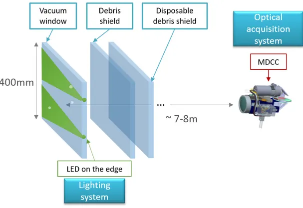
The experiment chamber of the LMJ facility is an 8 m in radius sphere. Eventually, 176 fused silica vacuum windows, distributed in quads over the sphere surface, will be analyzed after each laser shot. The MDCC imaging system is placed at the center by a motorized arm. This arm orients the MDCC toward each window. The image is formed on the sensor by a 6-lens objective optimized for the 525 nm wavelength. The pixel size of the MDCC projected onto the window plane is about 100 µm. The definition of the MDCC camera is 16 Mpixels. The CCD sensor is cooled at −25 °C in order to reduce thermal noise. The configuration of the MDCC system is presented in Figure1.
Figure 1: Configuration of the final optics assembly of the LMJ facility and position of MDCC when it is used to acquire images of a vacuum window from the chamber center.
To make laser damage sites visible, two green LEDs, with a maximum emissivity at 525 nm, are placed near one edge of each vacuum window. Light provided by LEDs enters into the optics and illuminates rear and front sides of the component. Laser damage sites, which are distributed on the front side of windows, scatter light. A part of the scattered light from damage sites is collected by the MDCC camera, which is focused on the front side of the vacuum window. The depth of field in the object space, which is equal to 15 mm, is sufficiently small to image only the front side of the window so that damage sites are sharp. Imaging of the vacuum window is possible through the debris shield and disposable debris shield but any damage on these optics may generate background noise and make detection of damage sites in vacuum windows more difficult.
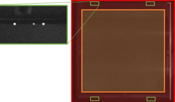
An example of a window image acquired by the MDCC camera is shown in Figure2. Laser damage sites are observed as well as light beams emitted by green LEDs, and reflections from mechanical objects around the window. However, the positioning of the MDCC is not perfect and illumination conditions may vary from one acquisition to another. To follow damage growth in series of acquisitions, it is necessary to correct small motions and intensity variations in image series.
Figure 2: Window image acquired by the MDCC. The two green LEDs near the left edge of the window illuminate the inside of the optical component. Laser-induced damage sites are revealed as small bright spots. Some reflections from mechanical objects and light sources located outside the experiment chamber are also visible.
Any image of a vacuum window (Figure3) is divided into different areas. Each area has specific features. The central area of vacuum windows, corresponding to the zone where the beam propagates through the window, is referred to as laser beam area. In that area, there are features such as laser damage sites that are likely to grow from shot to shot. The regular situation corresponds to vacuum windows free of any damage sites (Figure3). Successive shots will induce gradually more numerous damage sites in the laser beam area. Data from the laser beam area are therefore not sufficiently stable over time to be used for image registration. This zone represents more than 75% of the imaged area.
Figure 3: Different areas in a window image. The green box shows the four fiducial areas used for image registration. The red edge area contains the four fiducial areas. The orange laser beam area shows the region where the laser beam traverses the vacuum window.
Ideally, image registration should mainly use the remaining area, defined as edge area. The edge area contains
fiducial areas, divided into four zones located near each corner. Four reference “points,” designated as fiducials,
are located in each fiducial area. They are used as spatial markers to check the focusing plane of the MDCC on optics mostly free of any scratches, defects or damage sites. A fiducial is a crater made by ablation with a 𝐶𝑂2laser after optical polishing and before anti-reflective coating. Fiducial areas are also to used as reliable spots for image registration purposes. When a window is illuminated by the two LEDs located near one edge, each fiducial scatters sufficiently light toward the MDCC camera for being visible on images. Due to their position outside the laser beam
area, the fiducials are stable contrary to objects located inside the laser beam area. Gray levels of pixels belonging to edge areasare modified by light reflections from mechanical objects such as the aluminum alloy frame maintaining
the vacuum window. Variations of the lighting system induce gray level changes near image edges. Kinematic measurements cannot be performed securely in the laser beam area for two main reasons:
(i) In some situations, damage sites are not observed in the laser beam area. It is particularly true for new optics that have just been installed (Figure3). Consequently, no contrast is available for image registration.
(ii) After each laser shot, damage sites may initiate and others grow. Consequently, the assumption of gray level conservation is not satisfied even if background corrections are performed. Such effects make displacement estimations less secure.
Standard DIC codes are generally applied to images of speckled sample surfaces [25]. This speckle pattern provides sufficient contrast over the region of interest to ensure convergence of these codes. However, vacuum windows cannot be painted for obvious optical considerations. For all these reasons, displacement estimations by DIC were only per-formed on the fiducial areas and then extrapolated over the laser beam area thanks to the use of a reduced basis. It is worth noting that the fiducial areas used for registration purposes only represent about 0.7% of the total image area and surround the laser beam area.
Despite the fact that the location of vacuum windows is fixed, apparent ”motions” between successive LMJ vacuum window image acquisitions possess the following features:
• Translations up to tens of pixels.
• Rotations from some degrees up to 180°. Large rotations are due to the ad-hoc maintenance of the observation system that may lead to inversion of the camera frame.
• Limited scale changes close to one.
Such small displacement levels are due to small errors in repositioning of the MDCC system between successive image acquisitions. They occur between each acquisition of the same window. On the contrary, large rotations are (very) occasional. They are due to the maintenance of the observation system for example. From one acquisition to another, lighting conditions may change. The gray level variations are due to two phenomena:
• illumination variations of LEDs. They may slightly move and/or their intensity vary from one day to another. This phenomenon induces contrast changes between successive images. In the worst case, one LED can even be turned off.
• variations of other lighting sources near the experiment chamber. This phenomenon essentially induces non-uniform and unstable brightness variations.
These modifications lead to gray level variations and avoid an efficient comparison of images of the same window shot after shot.
Therefore damage tracking over time is highly dependent on the conditions associated with image acquisition. To be able to track efficiently damage sites, it is proposed to correct variations between successive images of the same optics.
3. Image registration and gray level correction
An algorithm is proposed to spatially register window images and correct for illumination variations. The algorithm begins with image registration using a DIC algorithm initialized by a first estimation of rigid body translations and rotation, in addition to scale changes. Once the registration is performed, gray level variations are corrected. DIC consists in estimating the displacement field by registering a reference image, 𝑓, and a deformed image of the scene, 𝑔.
Pixel coordinates in the image are denoted by 𝐱. The initial global residual 𝜏𝑖𝑛𝑖𝑡calculated over the considered Region
Of Interest (ROI) reads
𝜏𝑖𝑛𝑖𝑡2 = ∑
𝐱∈ROI
𝜌2𝑖𝑛𝑖𝑡(𝐱) with 𝜌𝑖𝑛𝑖𝑡(𝐱) = 𝑓 (𝐱) − 𝑔(𝐱) (1) where 𝜌 is the residual evaluated at each pixel position in the ROI. Considering window images, “disturbances” such as displacements (𝐮), illumination variations (brightness 𝑏 and contrast 𝑐), damage initiation and growth (𝑑) and ac-quisition noise (𝜂) have an effect on the initial residual
𝜌𝑖𝑛𝑖𝑡(𝐱) = 𝜌𝑖𝑛𝑖𝑡[𝐮(𝐱), 𝑏(𝐱), 𝑐(𝐱), 𝑑(𝐱)] + 𝜂(𝐱). (2)
The aim of this section is to describe a method that leads to a final residual value, 𝜌𝑓 𝑖𝑛𝑎𝑙, that only depends on gray
level variations due to damage sites and acquisition noise
𝜌𝑓 𝑖𝑛𝑎𝑙(𝐱) = 𝜌𝑓 𝑖𝑛𝑎𝑙(𝑑(𝐱)) + 𝜂(𝐱) (3)
3.1. Image registration
The first step of the method is to spatially register images. The hypothesis of local gray level conservation [25] reads
𝑓(x) = 𝑔(x + u(x)) (4)
where 𝐮 is the displacement field between the reference image 𝑓 and the deformed image 𝑔. For final optics images, this hypothesis is not exactly true due to illumination variations. Because of the stability of fiducials over time, it is assumed that the gray level variation is small enough in fiducial areas between successive images to consider the hypothesis of local gray level conservation valid at the registration step. Consequently, the DIC residual reads
𝜌𝐷𝐼 𝐶(𝐱) = 𝑓 (x) − 𝑔(x + u(x)) (5)
For vacuum window images, the displacement field is written as a linear combination of horizontal translation (𝑝 = 1), vertical translation (𝑝 = 2), rotation about the optical axis (𝑝 = 3) and scaling (𝑝 = 4)
𝐮(𝐱) = 4 ∑
𝑝=1
ΦΦΦ𝑝(𝐱, 𝜐𝑝) (6)
where the four fields 𝜙𝜙𝜙𝑝 are detailed in Table1. The four degrees of freedom correspond to those of similarity
trans-formations, which are a specific case of homography transformations [32]. Three of these fields (i.e., 𝑝 = 1, 2, 4) are linear with respect to the sought amplitudes 𝜐𝑝(i.e., ΦΦΦ𝑝(𝐱, 𝜐𝑝) = 𝜐𝑝𝜙𝜙𝜙𝑝(𝐱)). The third field (i.e., 𝑝 = 3) associated with
possibly large rotations is nonlinear in terms of the angular amplitude 𝜐3= 𝜃
Φ
where [𝐑(𝜃)] denotes the rotation matrix.
Table 1
Considered kinematic basis used to estimate displacement fields induced by MDCC motions.
Elementary displacement Field
Horizontal translation 𝜙𝜙𝜙1(𝐱) = 𝐞𝑥
Vertical translation 𝜙𝜙𝜙2(𝐱) = 𝐞𝑦
Rotation about optical axis ΦΦΦ3(𝐱, 𝜐3) = ([𝐑(𝜐3)] − [𝐈])𝐱
Scaling 𝜙𝜙𝜙4(𝐱) = 𝐱
The registration residual, 𝜏𝐷𝐼 𝐶, is defined as
𝜏𝐷𝐼 𝐶2 ({𝜐𝜐𝜐}) = ∑
x∈ROIDIC
𝜌2𝐷𝐼 𝐶(𝐱, {𝜐𝜐𝜐}) (8)
where ROIDICdefines the area used to estimate the displacement field 𝐮 (i.e., fiducial area, see Figure3). The aim of the registration algorithm is to find the four amplitudes 𝜐𝑖 that minimize 𝜏𝐷𝐼 𝐶2 over ROIDIC. This minimization
follows an iterative Gauss-Newton scheme [33]. A cubic interpolation scheme is used to create the corrected images. The iterative scheme of the minimization procedure ends when the norm of the iterative corrections is less than a determined threshold (i.e., 10−3px in the present case). At convergence, a registered image 𝑔
𝐷𝐼 𝐶is created.
The registration is simultaneously performed over the four fiducial areas (Figure3). As such, this is a global approach to DIC. Further, the selected kinematic basis only consists of four fields that were tailored to the present situation. It thus is an integrated DIC approach that does not require any additional post-processing once the four degrees of freedom were measured. In particular, they are easily extrapolated over the laser beam area.
It is necessary to choose initial values for the four amplitudes in order to initialize the first iteration of the min-imization scheme. One of the classical initializations, namely, starting with zero amplitudes, is not sufficient for window images because images may suffer from very large displacements due to large rotations as explained in Sec-tion2. An efficient initialization is essential to ensure the convergence of the registration algorithm [34,35]. Cross-correlation methods via Fast Fourier Transforms (FFT) are used to find these initial displacements, rotations and scale changes [36,37,38,39,40]. Each step of the initialization procedure is described in Figure4.
Figure 4: Different initialization steps of the registration.
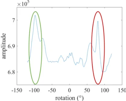
The first step consists in estimating the rotation of the deformed image 𝑔 with respect to the reference image 𝑓. Initially, images are encoded with Cartesian coordinates. Encoding Fourier transform images from Cartesian space to polar coordinates converts rotations into translations. A global correlation product is applied between the Fourier transforms of images 𝑓 and 𝑔 encoded in polar coordinates. This correlation product is translation invariant. The position of the peak of the correlation product gives the rotation angle between 𝑔 and 𝑓 [39]. However, the Fourier spectra of the images are centro-symmetric. The result of the correlation product is composed of two twin-peaks having the same maximum levels (Figure5). This phenomenon induces a 180-degree ambiguity [41]. After the estimation of the rotation, two angles are possible, 𝜃1and 𝜃2. This ambiguity is solved by the Displacement field selection step.
Figure 5: Cross-section of the correlation product of the Fourier spectrum encoded in polar space for a −100° angle. The green peak corresponds to the −100° angle and the red peak corresponds to the 80° angle (i.e., 80 ≡ −100° mod [180°]).
After the estimation of the rotation angle, the image 𝑔 is corrected with the two estimated angles, 𝜃1and 𝜃2. Scaling and translations are estimated using a correlation product in Cartesian frame between image 𝑓 and the images corrected by the two angles. The two images are separated in four quadrants corresponding to the four fiducial areas. The cross-correlation product is calculated on each quadrant of images encoded in Cartesian coordinates. A displacement vector is obtained for each quadrant, from which overall translations and scaling are deduced. The last step of the initialization procedure is the selection of the appropriate displacement field among the two options. The criterion consists in choosing the smallest residual between 𝜏1and 𝜏2computed over ROIGLcorresponding to the whole image except the edges.
The gray level residual after registration depends on gray level variations, damage growth and noise
𝜌𝐷𝐼 𝐶(𝐱) = 𝜌𝐷𝐼 𝐶[𝑏(𝐱), 𝑐(𝐱), 𝑑(𝐱)] + 𝜂(𝐱) (9)
Once the deformed image is corrected by the measured displacement field, the next step is to correct for gray level variations.
3.2. Brightness and Contrast Corrections
The gray level correction is estimated between the reference image 𝑓 and the corrected image 𝑔𝐷𝐼 𝐶. Gray level
variations between 𝑓 and 𝑔𝐷𝐼 𝐶are accounted for by performing brightness and contrast corrections [33]
where 𝑏 is the brightness field, and 𝑐 the contrast field. Consequently, the associated residual becomes
𝜌𝐺𝐿(𝐱) = 𝑓 (𝐱) − 𝑏(𝐱) − (1 + 𝑐(𝐱))𝑔𝐷𝐼 𝐶(𝐱) (11)
The brightness and contrast fields are written as linear combinations of new scalar fields 𝜓𝑘
𝑏(𝐱) = 𝑁 ∑ 𝑘=1 𝑏𝑘𝜓𝑘(𝐱) and 𝑐(𝐱) = 𝑁 ∑ 𝑘=1 𝑐𝑘𝜓𝑘(𝐱) (12)
where 𝑏𝑘 and 𝑐𝑘are the amplitudes to be determined. Contrary to the existing corrections for local DIC, which are
uniform over each considered subset [25], the brightness and contrast corrections are fields made up of low order polynomials since the laser beam area covers a large part of the image (see Table2). The low order polynomials do not remove the damage data.
Table 2
Interpolation fields, 𝜓𝑘, used for brightness and contrast corrections. The fields are expressed in dimensionless coordinates (𝑋, 𝑌 ) whose origin is the top left corner.
Order Interpolation fields
Constant 𝜓1(𝐱) = 1 Linear 𝜓2(𝐱) = 𝑋 𝜓3(𝐱) = 𝑌 Bi-linear 𝜓4(𝐱) = 𝑋𝑌 Order 2 𝜓5(𝐱) = 𝑋2 𝜓 6(𝐱) = 𝑌 2 ⋮ ⋮
Such corrections consist in solving a linear system in order to minimize the residual 𝜏𝐺𝐿
𝜏𝐺𝐿({𝐛}, {𝐜}) = ∑
𝐱∈ROIGL
𝜌2𝐺𝐿(𝐱, {𝐛}, {𝐜}) (13)
with respect to the amplitudes {𝐛}, {𝐜} of 𝑏 and 𝑐 fields, where ROIGLis defined as the beam area enlarged by 100 pixels on each edge (Figure3).
After solving the linear system, brightness and contrast fields are applied to image 𝑔𝐷𝐼 𝐶in order to get a registered
then only depends on damage variations and acquisition noise
𝜌𝐷(𝐱) = 𝜌𝐷(𝑑(𝐱)) + 𝜂(𝐱). (14)
4. Validation of proposed algorithm
An artificial image set was created in order to validate the previous algorithm.
4.1. Registration scheme
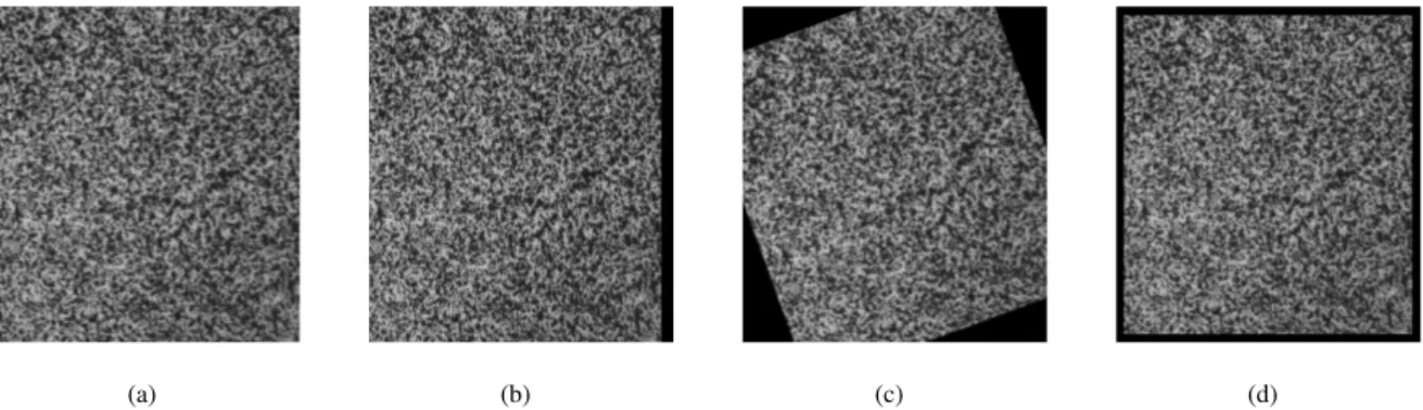
The reference image, 𝑓, is a black and white speckle pattern of a biaxial experiment on a low-cost composite [42]. To create the validation image set, displacements were applied to the reference image, 𝑓. The applied displacements correspond to typical motions that can be seen on vacuum window images. Images belonging to the validation set are shown in Figure6.
(a) (b) (c) (d)
Figure 6: Computer generated images used to validate the registration algorithm. (a) reference image. (b) −20.33 pixel horizontal translation. (c) −20° rotation. (d) Scaling with 0.95 factor.
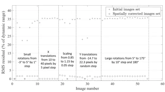
The validation image set of the registration algorithm is organized as follows: • Image 1: reference image
• Images 2 to 10: small rotations ranging from −3° to 5° by 1° step
• Images 11 to 18: translations along 𝐞𝑥from −10 to −40 pixels by 5-pixel step
• Images 19 to 25: scaling from 0.85 to 1.15 by 0.05 step
• Images 26 to 35: translations along 𝐞𝑦varying between 14.7 and −22.3 pixels by random steps
• Images 36 to 54: large rotations from 5° to 180°.
Figure7 shows the efficiency of image registration for all the images belonging to the validation set. Before registration, the mean RMS residual is 31% of the dynamic range of the reference image 𝑓. After registration, the mean RMS residual reaches 1.1%. If the displacement corrections were perfect, the residual should be exactly 0. The remaining difference comes from the cubic interpolation used for the creation of the validation images and the
correction of the deformed images. The residual is exactly 0 for images 11 to 18. For these images, no interpolation was needed since translations were integer-valued. This observation also applies for a 180° rotation and unitary scaling.
Figure 7: Dimensionless RMS residual before and after registration of the images belonging to the validation image set.
4.2. Gray level correction
For gray level correction, a validation image 𝑔𝑡𝑒𝑠𝑡is created from a brightness and contrast variation applied to the
reference image 𝑓 (with no additional motions)
𝑔𝑡𝑒𝑠𝑡(𝐱) = 𝑏𝑡𝑒𝑠𝑡(𝐱) + 𝑐𝑡𝑒𝑠𝑡(𝐱)𝑓 (𝐱) (15) with 𝑏𝑡𝑒𝑠𝑡(𝐱) = 10 sin (2𝜋𝐱 400 ) and 𝑐𝑡𝑒𝑠𝑡(𝐱) = 1 + 0.2 sin (2𝜋𝐱 400 ) (16)
The chosen brightness and contrast fields represent an approximation of an intensity increase of the two LEDs used to illuminate a vacuum window. It is worth noting that the selected fields do not belong to the assumed basis (see Table2). Images 𝑓 and 𝑔𝑡𝑒𝑠𝑡and the gray level corrected image (8 bit digitization) are shown in Figure8. The initial
(a) (b)
(c) (d)
(e) (f)
Figure 8: (a) Reference image 𝑓 , (b) validation image 𝑔𝑡𝑒𝑠𝑡, (c) corrected image 𝑔𝐺𝐿, and associated profiles for each image.
validation image. One can notice in Figure8a slight edge effect on 𝑔𝑡𝑒𝑠𝑡after gray level correction. In this example,
the ROI used for the correction corresponds to the whole image. To avoid this edge effect on the beam area of window images, ROIGLis the beam area enlarged by 100 pixels on each edge.
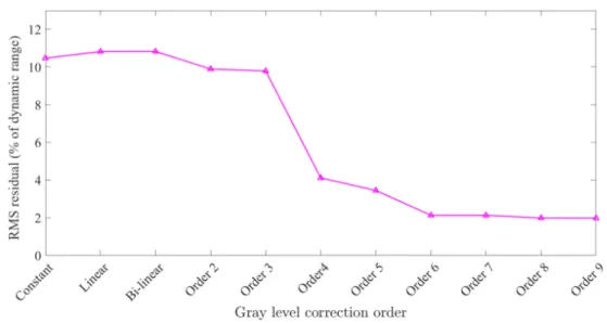
In Figure9, the influence of the order to correct gray level variations is investigated. If the field order is not sufficient, the RMS residual does not decrease and the gray level correction is not efficient. From order 4 on, the correction becomes useful. A satisfying correction is obtained from order 6 on and the gain becomes negligible for higher orders.
Figure 9: Influence of the scalar field order on the efficiency of the gray level correction for the selected fields.
5. Application to window images
The algorithm of image registration and gray level correction was validated on a set of computer-generated images. In this section, it is proposed to apply the developed procedure to an LMJ series of 18 vacuum window images acquired after laser shots. The main challenge lies in the “disturbances” between window images. They are mainly made of light reflections and noise that are not stable over time contrary to the speckle pattern of the computer generated images. As explained in Section2, fiducials located at each corner of vacuum windows were designed to help image registration. It will be shown that the four fiducial areas are sufficient to register vacuum window images and that gray level corrections applied to registered images is efficient. The effectiveness of the corrections is evaluated with the change of the RMS residual calculated over the ROI corresponding to the laser beam area, and on residual maps focus on a randomly selected laser damage located on the laser beam area.
Due to acquisition noise, the minimum residual level is 0.04% of the dynamic range of the reference image. The standard deviation of the noise was estimated on a 100 × 100-pixel (undamaged) area of the image over which the
average gray level was stable. The standard deviation of acquisition noise is equal 10 gray levels, and the root mean square corresponds to 0.04% of the dynamic range of the reference image. If the RMS residual level is greater than this threshold, one can state that something has changed between reference and deformed images. Initially, it could be small motions, gray level variations due to lighting conditions, or damage as described in Equation (2).
5.1. DIC registration
Results of the registration residuals are shown in Figure10. The initial residual levels are not stable over time due to all possible disturbances that can vary from an image to another. All RMS residuals are greater than the 0.04% threshold. The residual maps obtained before image registration show that motions actually occur. Image registration reduces the residual levels for images acquired after each laser shot. Residual maps obtained after image registration confirm that the registration is efficient as laser damage in the reference image is superimposed with the same laser damage on the registered image. Laser damage is still observable on the residual maps because its gray levels have changed between the reference configuration and the following acquisitions. Only residual maps after shots 2 and 18 are shown but the same results are observed over time.
Figure 10: Dimensionless RMS residuals before registration of MDCC images (dashed black line) are always higher than those obtained after image registration (dashed blue line). Residual maps corresponding to a damaged area are shown to confirm that image registration was efficient.
The RMS residuals are still greater than the 0.04% threshold due to acquisition noise. These levels could be due to variable lighting conditions and/or damage growth.
5.2. Gray level correction
The residual field after image registration mainly contains gray level variations due to illumination changes, damage growth and noise (Figure10). In this section, the proposed gray level correction is performed. It is essential that the gray level correction preserve damage data contained in residual maps. Results of the gray level correction are shown in Figure11. The chosen order for brightness and contrast fields is 𝑁 = 3.
The RMS residual before and after gray level correction is a good indicator of the effectiveness of the proposed correction. The final residual levels after both corrections oscillate between 0.05% and 0.13% of the dynamic range. This residual is very close to the 0.04% threshold due to acquisition noise, more stable and lower than those obtained after image registration alone. The residual maps in Figure11show that the gray level correction is effective to correct for variations due to variable illumination conditions.
Figure 11: Comparison of initial residual (dashed black line), residual after image registration (dashed blue line) and gray level variation (dashed red line) for the raw window images. The final residuals are significantly lower than their initial levels. Residual maps corresponding to a damage area are plotted in this figure in order to visually confirm that the corrections were efficient.
In Figure12, the influence of the scalar field order is studied for the gray level corrections. Constant brightness and contrast corrections over the laser beam area, which are equivalent to the so-called zero-mean normalized correc-tion [25,43], are not sufficient to take into account gray level variations on vacuum window images. Corrections of order 3 are a good compromise between correcting variations and keeping damage data (Figure13). More local vari-ations may lead to even lower residuals. Finite element discretizvari-ations [44] or principal component analyses [45] may be investigated. For the feasibility study performed herein, it is believed that the 3𝑟𝑑order corrections were sufficient.
Figure 12: Influence of the order of the scalar fields on the RMS residual.
Figure13shows the effectiveness of the gray level correction applied to the window image set. After brightness and contrast corrections, the profile of image 3 follows nearly that of the reference image without erasing the damage site. The brightness and contrast corrections significantly reduced the effect of illumination variations. However, the proposed method is not perfect. For instance, between 𝑌 coordinates 2500 and 3000 pixels of Figure13, there is still a difference between both profiles. One can notice that in this section, the variation is less than 50 gray levels, close to acquisition noise.
Figure 13: Profile comparison of image 3 after registration, after brightness and contrast corrections, and reference image. The narrow peak corresponds to a damage site that is preserved by the various corrections.
5.3. Preliminary brightness correction
Up to now, the brightness and contrast corrections were performed after spatial registrations on raw dark-field images. In order to enhance the effectiveness of the gray level corrections, a preliminary correction is proposed. After each shot, two different images of a vacuum window are acquired:
• A window image with LEDs turned on. In this image, scattering objects located on the window are visible. An illumination variation caused by the LEDs induces contrast variations from one image to another.
• A window image with LEDs turned off. The aim of this acquisition is to get all the illumination effects coming from all other sources than LEDs. Such sources, which are not stable from one acquisition to another, lead to brightness variations.
The difference between these two images makes it possible to create pre-corrected images that may have the same brightness level from one acquisition to another. This pre-correction slightly enhances the brightness and contrast corrections as shown in Figure14. Thanks to this operation, the hypothesis of gray level conservation, which is used for image registration, is more valid and image registration is likely to be more stable.
Figure 14: Comparison of initial residual, after image registration, residual, after brightness and contrast corrections for raw images and pre-corrected images.
An increase of the RMS residuals for pre-corrected images between shot 9 and 10 before gray level correction may be due to illumination issues. An analysis of the contrast field for images from shots 9 and 10 (Figure15) proves that the sudden increase before gray level corrections is due to the bottom LED. In that area, the contrast level is close to one for image from shot 9 and tends to zero for image from shot 10. It is possible to state that the bottom LED was turned off before image from shot 10. This conclusion is confirmed by the observation of registered images from shots 9 and 10, in Figure15. In that area, the gray levels increased between images from shots 9 and 10.
(a) (b)
(c) (d)
Figure 15: Effect of turning on an LED on the estimated contrast field (see green ellipses). (a,b) Estimated contrast field for image from shots 9 (a) and 10 (b) subtracted by the image from shots 9 and 10 respectively acquired with LED off. (c,d) Registered image from shots 9 (c) and 10 (d) subtracted by the image from shots 9 and 10 respectively acquired with LED off.
The brightness and contrast corrections make comparisons between corrected images after each shot possible. The detection of abnormal illumination variations (e.g., turning on and off LEDs) is also possible thanks to an analysis of the contrast field. When an LED is switched off during image acquisition, the luminance near that LED is too weak to make damage sites in this area visible. It is essential to check that the LEDs are turned on to be able to detect and follow damage growth from one shot to another. Brightness and contrast corrections account for illumination variations but they cannot find missing information (in too dark zones).
Except for an exceptional issue related to LEDs, the proposed algorithms make Lagrangian comparisons of suc-cessive images possible. After image registration and gray level corrections, the residual only depends on damage initiation and growth, as well as acquisition noise.
6. Laser damage detection and quantification
Once the window images are corrected thanks to the presented algorithms, it is possible to compare directly gray levels of successive images. In these conditions, each gray level variation that is more important than noise can be considered as a potential damage site. Based on this observation, an efficient way to detect potential damage sites and to quantify damage growth is presented.
6.1. Detection of potential damage sites
To detect damage sites, it is proposed to threshold absolute values of residual maps 𝜌𝑖
𝐷𝐼 𝐶+𝐺𝐿between the reference image and the corrected image acquired after laser shot 𝑖, 𝑔𝑖
𝐷𝐼 𝐶+𝐺𝐿. This thresholding method is designated as DIC thresholding in the following part of this section. The detection threshold has to be small enough to capture all damage sites as soon as they initiate. However, the selected threshold has to be higher than acquisition noise to avoid numerous false alarms. Experimentally, acquisition noise was estimated to have a standard deviation of 10 gray levels.
The present approach is compared to LASNR that does not take into account the evolution of gray levels over time, contrary to the present method. The detection principle of the LASNR method is based on the comparison of the grey level of each pixel with its surrounding neighbors [23].
Figure16shows all detected sites on the same image with both analyses. The DIC threshold is defined at the acquisition noise limit. The LASNR parameters are the same as those used on LMJ. With these parameters, DIC is more efficient than LASNR to detect potential damage sites. The former detects twice the number of objects than the latter for the treated example. Undetected sites by LASNR are isolated pixels that have a varying gray level near acquisition noise of the observation system. The proposed approach can be considered as more efficient than LASNR as it detects objects that initiate and grow from one shot to another.
Figure 16:Results of two different detection methods. On the left, detected sites by LASNR. On the right, sites determined via DIC. The detected damage sites are represented by white boxes. The selected area used to illustrate damage growth is depicted as the red box.
If the reference image were acquired on an undamaged window, all initiated damage sites would possibly be de-tected by DIC as soon as their gray levels are higher than that corresponding to acquisition noise of the camera.
6.2. Damage growth
It is necessary to know if detected objects are truly laser-induced damage sites or any other object. The labeling of detected sites as damaged is possible by following the change of the residual 𝜌𝐷of an area around them. An example
corresponding to a detected site (red box in Figure16) is chosen to illustrate this section. The aim is to be sure that detected zones by DIC are actually damage sites, and to quantify damage growth after each shot.
An estimation of the maximum diameter of damage sites is approximately equal to one millimeter. This size is equivalent to tens of pixels on images. Therefore, an analysis area of 50-pixel side centered about each detected site is defined. In order to identify laser damage sites among all detected areas, an analysis of the RMS residual for each of them is performed. Dust and other particles are not bonded on the window. They may disappear or move from an acquisition to another. This phenomenon leads to a brief increase of the RMS residual, and then a decrease to initial levels. Objects associated with this feature are not damage sites.
The quantification of damage growth is carried out with the analysis of the variation of the RMS residual on the selected area. Figure17shows the change of the residual map from the first to the last image for the area under study. The size and gray level of the damaged zone increase after each shot. However, damage growth is not constant.
(a) (b) (c)
(d) (e) (f)
(g) (h)
Figure 17: Variation of gray level residual maps after each shot on the analysis area selected for a detected damage site (red box in Figure16) with DIC for shots 1 (a), 2 (b), 4 (c), 6 (d), 8 (e), 12 (f), 14 (g), 16 (h). The image is encoded over 16 bits.
The increase of RMS residual after each shot is compared to the energy level of the corresponding shot in Figure18. It is observed that:
• The increase of RMS residual is linked with the growth of the damaged area. These gray levels are directly connected with the way damage sites scatter light.
• The variation of RMS residual is potentially related to the energy at 3𝜔 of the corresponding shot [6]. In the studied example, the RMS level does not change when the energy of the shot is less than 2 kJ. Conversely, it increases when the energy is of the order of 3 kJ. It is worth noting that the residual estimated for the damaged area is local in comparison to the shot energy that is global, namely, calculated for the whole beam. Furthermore,
other parameters, such as pulse duration, may have an influence on damage growth on vacuum windows [6]. A statistical analysis on more damage sites and shots is necessary to analyze such correlations.
Figure 18: Variation of RMS residual for the analyzed area (displayed in Figure17) after each shot. Comparison with the global energy of each shot.
7. Conclusion
In this paper, a solution for spatial registration and correction of illumination variations was presented for the detection of damage on LMJ vacuum windows. Special implementations were required since the area over which DIC was performed was not identical to that where brightness/contrast corrections were carried out. A reduced kinematic basis was selected to extrapolate the measured displacement fields. The proposed algorithms were first validated on computer-simulated images using a standard speckle pattern for DIC analyses. Then, they were applied to a set of real images of an LMJ vacuum window where fiducials were used for registration purposes, and the beam illuminated area for brightness and contrast corrections.
The proposed correction methods can be used in high energy laser facilities where it is necessary to follow damage growth in which small motions and illumination variations may occur. The new method of laser-induced damage detection is based on the analysis of the final residual fields. Detection and quantification of laser-induced damage led to very low residual levels as functions of laser shots. These residual maps are independent of the displacements between acquisitions and are no longer affected by gray level variations that are not induced by damage growth. The present implementation was compared to the widely-used LASNR algorithm and provided better results. The advantage of this method is to be based on the overall increase of light scattering with damage growth.
with the aim of identifying factors modifying the scattering level of damage sites. The gray levels of damage sites may then be linked with their size as well as the fracture mechanism or with the morphology of the crater.
Acknowledgements
The authors thank Nicolas Bonod and Sébastien Vermersch for useful and interesting discussions.
Declaration of Competing Interest
The authors declare that they have no known competing financial interests or personal relationships that could have appeared to influence the work reported in this paper.
CRediT authorship contribution statement
Guillaume Hallo:Conceptualization, Methodology, Software, Writing - Original Draft. Chloé Lacombe:Resources, Writing - Review & Editing.
Jérôme Néauport:Funding acquisition, Writing - Review & Editing.
François Hild: Conceptualization, Methodology, Validation, Supervision, Writing - Review & Editing.
References
[1] M. L. Andre, “Status of the LMJ project,” in Solid State Lasers for Application to Inertial Confinement Fusion: Second Annual International Conference (M. L. Andre, ed.), vol. 3047, pp. 38 – 42, International Society for Optics and Photonics, SPIE, 1997.
[2] J. A. Paisner, E. M. Campbell, and W. J. Hogan, “The national ignition facility project,” Fusion Technology, vol. 26, 11 1994. [3] W. Hogan, E. Moses, B. Warner, M. Sorem, and J. Soures, “The national ignition facility,” Nuclear Fusion, vol. 41, p. 567, 05 2002. [4] W. Zheng, X. Wei, Q. Zhu, F. Jing, D. Hu, J. Su, and et al., “Laser performance of the sg-iii laser facility,” High Power Laser Science and
Engineering, vol. 4, p. e21, 2016.
[5] H. Schwoerer, J. Magill, and B. Beleites, Lasers and Nuclei. Springer, 2006.
[6] K. Manes, M. Spaeth, J. Adams, and M. Bowers, “Damage mechanisms avoided or managed for nif large optics,” Fusion Science and Technology, vol. 69, pp. 146–249, 02 2016.
[7] S. G. Demos, M. Staggs, and M. R. Kozlowski, “Investigation of processes leading to damage growth in optical materials for large-aperture lasers,” Applied Optics, vol. 41, pp. 3628–3633, 06 2002.
[8] M. Veinhard, O. Bonville, S. Bouillet, E. Bordenave, R. Courchinoux, R. Parreault, and et al., “Effect of non-linear amplification of phase and amplitude modulations on laser-induced damage of thick fused silica optics with large beams at 351 nm,” Journal of Applied Physics, vol. 124, p. 163106, 10 2018.
[9] N. Bloembergen, “Role of cracks, pores, and absorbing inclusions on laser induced damage threshold at surfaces of transparent dielectrics,” Applied Optics, vol. 12, pp. 661–664, 04 1973.
[10] J. Neauport, P. Cormont, P. Legros, C. Ambard, and J. Destribats, “Imaging subsurface damage of grinded fused silica optics by confocal fluorescence microscopy,” Optics Express, vol. 17, pp. 3543–3554, 03 2009.
[11] M. J. Soileau, W. E. Williams, N. Mansour, and E. W. V. Stryland, “Laser-Induced Damage And The Role Of Self-Focusing,” Optical Engineering, vol. 28, no. 10, pp. 1133 – 1144, 1989.
[12] D. M. Kane and D. R. Halfpenny, “Reduced threshold ultraviolet laser ablation of glass substrates with surface particle coverage: A mechanism for systematic surface laser damage,” Journal of Applied Physics, vol. 87, no. 9, pp. 4548–4552, 2000.
[13] S. Palmier, S. Garcia, L. Lamaignère, M. Loiseau, T. Donval, J. L. Rullier, and et al., “Surface particulate contamination of the LIL optical components and their evolution under laser irradiation,” in Laser-Induced Damage in Optical Materials: 2006 (G. J. Exarhos, A. H. Guenther, K. L. Lewis, D. Ristau, M. J. Soileau, and C. J. Stolz, eds.), vol. 6403, pp. 301 – 310, International Society for Optics and Photonics, SPIE, 2007.
[14] M. Chambonneau and L. Lamaignère, “Multi-wavelength growth of nanosecond laser-induced surface damage on fused silica gratings,” Scientific Reports, vol. 8, pp. 1–10, 01 2018.
[15] R. A. Negres, D. A. Cross, Z. M. Liao, M. J. Matthews, and C. W. Carr, “Growth model for laser-induced damage on the exit surface of fused silica under uv, ns laser irradiation,” Optics Express, vol. 22, pp. 3824–3844, 02 2014.
[16] R. A. Negres, M. A. Norton, D. A. Cross, and C. W. Carr, “Growth behavior of laser-induced damage on fused silica optics under uv, ns laser irradiation,” Optics Express, vol. 18, pp. 19966–19976, 09 2010.
[17] P. Cormont, P. Combis, L. Gallais, C. Hecquet, L. Lamaignère, and J. L. Rullier, “Removal of scratches on fused silica optics by using a co2 laser,” Optics Express, vol. 21, pp. 28272–28289, 11 2013.
[18] J. Folta, M. Nostrand, J. Honig, N. Wong, F. Ravizza, P. Geraghty, and et al., “Mitigation of laser damage on National Ignition Facility optics in volume production,” in Laser-Induced Damage in Optical Materials: 2013 (G. J. Exarhos, V. E. Gruzdev, J. A. Menapace, D. Ristau, and M. Soileau, eds.), vol. 8885, pp. 138 – 146, International Society for Optics and Photonics, SPIE, 2013.
[19] T. Doualle, L. Gallais, S. Monneret, S. Bouillet, A. Bourgeade, C. Ameil, and et al., “CO2 laser microprocessing for laser damage growth mitigation of fused silica optics,” Optical Engineering, vol. 56, no. 1, pp. 1 – 9, 2016.
[20] F. Wei, F. Chen, B. Liu, Z. Peng, J. Tang, Q. Zhu, and et al., “Automatic classification of true and false laser-induced damage in large aperture optics,” Optical Engineering, vol. 57, no. 5, pp. 1 – 11, 2018.
[21] L. Mascio-Kegelmeyer, “Machine learning for managing damage on NIF optics,” in Laser-induced Damage in Optical Materials 2020 (C. W. Carr, V. E. Gruzdev, D. Ristau, and C. S. Menoni, eds.), vol. 11514, International Society for Optics and Photonics, SPIE, 2020.
[22] C. Lacombe, S. Vermersch, G. Hallo, M. Sozet, P. Fourtillan, R. Diaz, and et al., “Dealing with LMJ final optics damage: post-processing and models,” in Laser-induced Damage in Optical Materials 2020 (C. W. Carr, V. E. Gruzdev, D. Ristau, and C. S. Menoni, eds.), vol. 11514, International Society for Optics and Photonics, SPIE, 2020.
[23] L. Kegelmeyer, P. Fong, S. Glenn, and J. Liebman, “Local area signal-to-noise ratio (lasnr) algorithm for image segmentation,” Proceedings of SPIE - The International Society for Optical Engineering, vol. 6696, 10 2007.
[24] C. Amorin, L. Kegelmeyer, and W. Kegelmeyer, “A hybrid deep learning architecture for classification of microscopic damage on national ignition facility laser optics,” Statistical Analysis and Data Mining: The ASA Data Science Journal, vol. 12, 09 2019.
[25] M. A. Sutton, J.-J. Orteu, and H. W. Schreier, Image Correlation for Shape, Motion and Deformation Measurements - Basic Concepts, Theory and Applications. Springer Science, 2009.
[26] P. Rastogi and E. Hack, Optical Methods for Solid Mechanics: A Full-Field Approach. Weinheim Wiley-VCH-Verl. 2012, 06 2012. [27] M. A. Sutton, “Computer Vision-Based, Noncontacting Deformation Measurements in Mechanics: A Generational Transformation,” Applied
Mechanics Reviews, vol. 65, 08 2013.
[29] F. Hild and S. Roux, Handbook of damage mechanics, ch. Evaluating Damage with Digital Image Correlation: A. Introductory Remarks and Detection of Physical Damage, pp. 1255–1275. Springer, 2015.
[30] E. Schwartz, R. Saralaya, J. Cuadra, K. Hazeli, P. A. Vanniamparambil, R. Carmi, and et al., “The use of digital image correlation for non-destructive and multi-scale damage quantification,” in Sensors and Smart Structures Technologies for Civil, Mechanical, and Aerospace Systems 2013 (J. P. Lynch, C.-B. Yun, and K.-W. Wang, eds.), vol. 8692, pp. 706 – 720, International Society for Optics and Photonics, SPIE, 2013.
[31] M. Mehdikhani, E. Steensels, A. Standaert, K. Vallons, L. Gorbatikh, and S. Lomov, “Multi-scale digital image correlation for detection and quantification of matrix cracks in carbon fiber composite laminates in the absence and presence of voids controlled by the cure cycle,” Composites Part B: Engineering, vol. 154, pp. 138–147, 12 2018.
[32] R. I. Hartley and A. Zisserman, Multiple View Geometry in Computer Vision. Cambridge University Press, ISBN: 0521540518, second ed., 2004.
[33] F. Hild and S. Roux, “Digital image correlation,” in Optical Methods for Solid Mechanics. A Full-Field Approach (P. Rastogi and E. Hack, eds.), (Weinheim (Germany)), pp. 183–228, Wiley-VCH, 2012.
[34] G. Besnard, F. Hild, and S. Roux, ““Finite-element” displacement fields analysis from digital images: Application to Portevin-Le Chatelier bands,” Experimental Mechanics, vol. 46, pp. 789–803, 2006.
[35] Z. Jiang, Q. Kemao, H. Miao, J. Yang, and L. Tang, “Path-independent digital image correlation with high accuracy, speed and robustness,” Optics and Lasers in Engineering, vol. 65, pp. 93–102, 2015. Special Issue on Digital Image Correlation.
[36] D. Barker and M. Fourney, “Measuring fluid velocities with speckle patterns,” Optics Lett., vol. 1, pp. 135–137, 1977. [37] T. Dudderar and P. Simpkins, “Laser speckle photography in a fluid medium,” Nature, vol. 270, pp. 45–47, 1977.
[38] R. Grousson and S. Mallick, “Study of flow pattern in a fluid by scattered laser light,” Applied Optics, vol. 16, pp. 2334–2336, 1977. [39] B. S. Reddy and B. N. Chatterji, “An fft-based technique for translation, rotation, and scale-invariant image registration,” IEEE Transactions
on Image Processing, vol. 5, pp. 1266–1271, 08 1996.
[40] Z. Fang, Y. Gao, Z. Gao, Y. Liu, Y. Wang, Y. Su, and Q. Zhang, “Efficient and automated initial value estimation in digital image correlation for large displacement, rotation, and scaling,” Appl. Opt., vol. 59, pp. 10523–10531, Nov 2020.
[41] J. N. Sarvaiya, S. Patnaik, and S. Bombaywala, “Image registration using log-polar transform and phase correlation,” in TENCON 2009 - 2009 IEEE Region 10 Conference, pp. 1–5, 01 2009.
[42] D. Claire, F. Hild, and S. Roux, “Identification of damage fields using kinematic measurements,” Comptes Rendus Mécanique, vol. 330, pp. 729–734, 2002.
[43] B. Wang, B. Pan, and G. Lubineau, “Some practical considerations in finite element-based digital image correlation,” Optics and Lasers in Engineering, vol. 73, pp. 22–32, 2015.
[44] V. Sciuti, R. Canto, J. Neggers, and F. Hild, “On the benefits of correcting brightness and contrast in global digital image correlation: Moni-toring cracks during curing and drying of a refractory castable,” Optics and Lasers in Engineering, vol. 136, p. 106316, 2021.
[45] C. Jailin and S. Roux, “Modal decomposition from partial measurements,” Comptes Rendus Mécanique, vol. 347, no. 11, pp. 863 – 872, 2019. [46] S. Liukaityte, M. Zerrad, M. Lequime, T. Bégou, and C. Amra, “Measurements of angular and spectral resolved scattering on complex optical coatings,” in Optical Systems Design 2015: Advances in Optical Thin Films V (M. Lequime, H. A. Macleod, and D. Ristau, eds.), vol. 9627, pp. 229 – 235, International Society for Optics and Photonics, SPIE, 2015.