HAL Id: hal-01344048
https://hal.archives-ouvertes.fr/hal-01344048
Submitted on 19 Jul 2016
HAL is a multi-disciplinary open access
archive for the deposit and dissemination of
sci-entific research documents, whether they are
pub-lished or not. The documents may come from
teaching and research institutions in France or
abroad, or from public or private research centers.
L’archive ouverte pluridisciplinaire HAL, est
destinée au dépôt et à la diffusion de documents
scientifiques de niveau recherche, publiés ou non,
émanant des établissements d’enseignement et de
recherche français ou étrangers, des laboratoires
publics ou privés.
Solving Problems with CP: Four Common Pitfalls to
Avoid
Jean-Charles Régin
To cite this version:
Jean-Charles Régin. Solving Problems with CP: Four Common Pitfalls to Avoid. CP 2011 - Principles
and Practice of Constraint Programming - 17th International Conference, Jimmy Ho-Man Lee, Sep
2011, Perugia, Italy. �10.1007/978-3-642-23786-7_3�. �hal-01344048�
Solving Problems with CP: Four Common
Pitfalls to Avoid
Jean-Charles R´egin
Universit´e de Nice-Sophia Antipolis, I3S UMR 6070, CNRS, France. [email protected]
Abstract. Constraint Programming (CP) is a general technique for solving combinatorial optimization problems. Real world problems are quite complex and solving them requires to divide work into different parts. Mainly, there are: the abstraction of interesting and relevant sub-parts, the definition of benchmarks and design of a global model and the application of a particular search strategy. We propose to identify for each of these parts some common pitfalls and to discuss them. We will successively consider undivided model, rigid search, biased benchmarking and wrong abstraction.
1
Introduction
The resolution of real world complex problems is hard for several reasons: the size of the problem, the intrinsic difficulty of some subparts and the combination of subparts. Therefore, it requires the implementation of a complex procedure divided into several steps. We can identify four of them. First, the user has to try to abstract some parts of the problem in order to focus his attention on difficult and relevant parts, or on combinations of these parts. Then, a bench-marking process must be defined in order to be able to work on smaller instances than the whole problem. This process is needed for ensuring that the previous step abstraction and the obtained results with small problems will be generally applicable. Next, a global model must be defined. Here, we mean the method that will be used for solving the whole problem and not each part. That is, for instance, the successive resolution of each part and their combination. At last, a search strategy is defined for the most important parts.
All these different aspects are well known. However, it appears that we tend to repeat the same mistakes. Hence, we propose to try to identify some pitfalls. We will show the benefit that we can obtain by avoiding them. For each step of the resolution process, we identify one strong pitfall and try to give it a pertinent name:
– undivided model – rigid search
– biased benchmarking – wrong abstraction
The undivided model pitfall means that the global model for solving the whole problem is too much general, in other words, we could certainly improve the resolution if we split the resolution into different parts.
The rigid search expresses the idea of a search strategy which is too much linked to a depth first search procedure. We should benefit from the recent re-search about random restart and avoid waiting too long in a wrong part of the search tree before leaving it.
The biased benchmarking corresponds to a process which cannot be globally applicable. In other words, the obtained results for the smaller problems that are considered could not be used to derive some global rules or ideas for solving the whole problem.
The wrong abstraction defines a wrong identification of a relevant subpart of the whole problem. For instance, the subpart may not include an important constraint and be easy to solve in this context, whereas in the whole problem the introduction of the missing constraint will totally change the difficulty.
We propose to detail these fours aspects
2
Undivided Model
Complex problems usually involve the combination of some other complex prob-lems. Thus, we have two possibilities: either we deal with the whole problem in one step, that is we integrate all the constraints and we try to solve the ob-tained problem, or we split the problem into different parts and then we solve the parts independently and we try to combine them. Note that the indepen-dent resolutions of the subparts may be relative. Classical MIP formulations and resolutions have nice examples of decompositions. The most well known are certainly column generation and Bender’s decomposition.
We propose to emphasize this point on a well known example in CP the sports scheduling problem of the MIPLIB which is described in [10]. A more recent and nice example of decomposition can be found in [8], where a load balancing problem must be solved.
The problem consists of scheduling games between n teams over n − 1 weeks. In addition, each week is divided into n/2 periods. The goal is to schedule a game for each period of every week so that the following constraints are satisfied:
1. Every team plays against every other team; 2. A team plays exactly once a week;
3. A team plays at most twice in the same period over the course of the season. The first two constraints just define a round robin. The third one complexifies the problem.
A solution to this problem for 8 teams is shown in Figure 1. The problem can be made more uniform by adding a ”dummy” final week and requesting that all teams play exactly twice in each period.
Week 1 Week 2 Week 3 Week 4 Week 5 Week 6 Week 7 period 1 0 vs 1 0 vs 2 4 vs 7 3 vs 6 3 vs 7 1 vs 5 2 vs 4 period 2 2 vs 3 1 vs 7 0 vs 3 5 vs 7 1 vs 4 0 vs 6 5 vs 6 period 3 4 vs 5 3 vs 5 1 vs 6 0 vs 4 2 vs 6 2 vs 7 0 vs 7 period 4 6 vs 7 4 vs 6 2 vs 5 1 vs 2 0 vs 5 3 vs 4 1 vs 3
Fig. 1: A solution to the Sports-Scheduling Application with 8 teams.
With the dummy column, the most efficient model seems to be the following one:
We use two classes of variables:
•team variables specifying the team playing on a given week, period and
slot;
•game variables specifying which game is played on a given week and period.
The use of game variables makes it simple to state the constraint that every team must play against each other team. Since games are uniquely identified by their two teams, there are n ∗ (n − 1)/2 possible values for the game vari-ables, and by defining an alldiff constraint on the game variables we ensure that the first constraint is satisfied. Team variables and game variables are simply linked by ternary table constraints given in extension. For each slot i, a table constraint involves the variables gi, thi, tai where gi is the game variable, thi
and tai the team variables of this slot. For 8 teams, it is defined by the list of
tuples < 1, 1, 2 >, < 2, 1, 3 >, ..., < 56, 7, 8 > where a combination < g, t1, t2 >
means that the game number g corresponds to the game t1vs t2. For each week,
the constraint on the week (constraint 2) is represented by an alldiff constraint involving the team variables of the week. For each period, the constraint on the period (constraint 3) is represented by a global cardinality constraint involving the team variable of the period.
We add an additional constraint for breaking symmetry: the game 0 vs w appears in week w. In addition, the search strategy is defined as follows. Teams are instantiated (that is value of team variables). We select the team which is the most instantiated and we select the team variable having this value in its domain and the smallest domain size and we assign this variable to this team value. Here are the results we obtain:
#teams #fails time (s) 8 32 0.08 10 417 0.8 12 41 0.2 14 3,514 9.2 16 1,112 4.2 18 8,756 36 20 72,095 338 24 6,391,470 12h
This model is a global one and it involves only one step: all the constraints are defined and we try to find a solution. The results are good but we can really improve them if we try to decompose the model. For instance, the link between rows and columns is an issue. In addition, this problem can be seen in a different way: we have to find a round robin which satisfies the period constraint. Thus, instead of trying to find a round robin and at the same time to satisfy the period constraint, we could try to decompose the problem into its two natural parts:
1. We compute a round robin, which is an easy task (i.e. a polynomial algo-rithm is available). This means that we satisfy the alldiff constraint on game variables and we satisfy all the constraints on team variables for each week. 2. Then, we try to rearrange the elements of each column such that the period
constraint is satisfied.
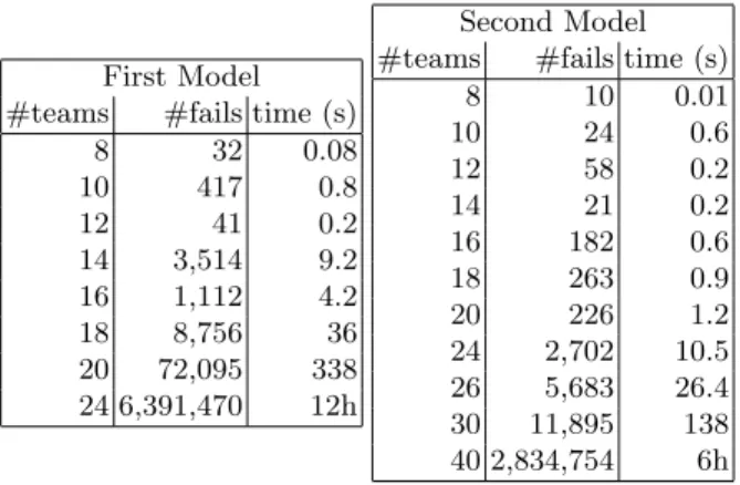
In this model, symmetries are broken by setting 0 vs 1 as the first game of the dummy column. Then, rows and columns are successively instantiated. The major risk of this decomposition is that there may be no way to satisfy the period constraints for the computed round robin. In this case, another round robin should be computed and so on... Fortunately, this is not the case, as shown by the obtained results given in Figure 2.
This example clearly shows that decomposition may lead to huge improve-ments. Note that the method we use is quite general: we precompute a solution for a part of the problem and we try to rearrange it in order to satisfy some additional constraints.
3
Rigid Search
At the beginning of CP, mainly static search strategies were considered. This means that the set of variables is ordered a priori, that is before starting the search. Then, the next assigned variable is selected w.r.t this order: the first non assigned variable is selected and a value is assigned to it. Then, dynamic orderings have been introduced. With dynamic orderings, the next variable to assign is computed. Generally, a criteria is defined and recomputed for each variable when a selection has to be made. The variable having the best value for this criteria is chosen as the next variable to assign. A lot of studies have been made and several orders have been proposed.
First Model #teams #fails time (s)
8 32 0.08 10 417 0.8 12 41 0.2 14 3,514 9.2 16 1,112 4.2 18 8,756 36 20 72,095 338 24 6,391,470 12h Second Model #teams #fails time (s)
8 10 0.01 10 24 0.6 12 58 0.2 14 21 0.2 16 182 0.6 18 263 0.9 20 226 1.2 24 2,702 10.5 26 5,683 26.4 30 11,895 138 40 2,834,754 6h
Fig. 2: The results obtained with two different models for solving sports schedul-ing problems.
In addition, the search space is usually traversed by a depth first search.
These methods work well for a lot of problems, however they have in general a huge drawback as it has been shown by C. Gomes et al [4] who emphasized heavy tails phenomena in quasigroup completion problem.
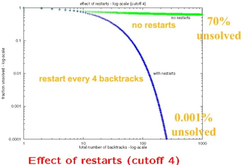
Heavy tails phenomena have been observed by Pareto in the 1920’s. A stan-dard distribution has an exponential decay, whereas a heavy tail distribution has a power law decay. This phenomena arises in a lot of problems and in constraint programming. For instance, while trying to solve some instances of the latin square completion problem, Gomes et al. discovered that there is no ordering which is able to solve all the instances in a short period of time. About 18% of the instances remain unsolvable even with 100, 000 backtracks. Then, they proved theoretically that heavy tail phenomena may be eliminated by using a strategy for selecting the next assignment which involves some randomness and by restarting the search when the solver begins to backtrack. The idea is very nice and quite simple. Roughly, the idea can be described as follows: when se-lecting a variable instead of taking the one having the best score in regards to some criteria, consider the 10% best variables and randomly select one among them. This is the selection method. Now, after a certain number of backtracks, we restart the search for a solution from scratch: this is the restart method. Figure 3 shows the effect of this method.
This method performs very well in practice and has been intensively used in commercial solvers like ILOG CP. It is also used by some MIP solvers. It encourages us to be careful with too much rigid search and to accept to be less deterministic.
Fig. 3: Impact of restarts (published with the courtesy of C. Gomes).
4
Biased Benchmarking
Identifying an interesting problem is a first step but not the only one. It is also quite important to design some benchmarks from which we could expect to derive general considerations. This part is not enough studied and may cause some problems because we have to make sure that the deduction may be still valid in general and not only for the particular instances we studied. Biased benchmarking represents the fact that the result obtained from a benchmark can be not representative of the whole problem. Biased benchmarking will prevent us from generalizing our results.
In other words, it means that benchmarks should not be too much focused on a very specific part of a more general problem. Unfortunately, this is not always the case. For instance, for the bin packing problem1, it appears that most of the instances proposed in the literature have some major drawbacks. Gent [3] criticized the well known Falkenauer’s benchmarks [2]. He closed five benchmark problems left open by cpu-intensive methods using a genetic algorithm and an exhaustive search method by using a very simple heuristic method requiring only some seconds of cpu time and hours of manual work. He questioned the under-lying hardness of test data sets. One reason of the problem is the kind of data sets: most of the time, bins are filled in with only 3 items or less. Unfortunately,
1
From Wikipedia: objects of different volumes must be packed into a finite number of bins of capacity V in a way that minimizes the number of bins used.
the same kind of data sets have been proposed by others [9, 6, 5]. Korf took it right up to explicitly consider triplets instances.
The issue here is not only the type of the data. It changes the kind of problem which is solved. With such data sets, we can only conclude about problems involving only few items per bins and not for the bin packing problem in general. In fact, if there are few items per bin, then the capacity constraints dominate the problems, whereas it is not the case when there are more items per bin. We can prove this by considering the set of solution of the Diophantine equation ax + by = c. If we consider the case where the greatest common divisor (gcd) is 1, then this equation has always a solution when ab ≥ c and a solution in half of the cases when ab < c (from Paoli’s theorem). If we consider now the equation ax + by + cz = d then we have less chance to have a gcd greater than 1 and the equation is equivalent to the system ax + by = d − c or ax + by = d − 2c or ... This means that the density of solutions increases. So, if several variables are involved, then the equation will have more chances to be satisfied. Since this equation corresponds to the sum constraint involved for each bin, this means that we have less and less chance to be able to filter the domains of the variables when the number of variables increases. Therefore, benchmarks for the bin packing problems should consider different types of data depending on the number of items per bin.
5
Wrong Abstraction
In general, it is difficult to identify the relevant subparts of a problem, that is the part that deserves a particular study. The wrong abstraction pitfall corresponds to the identification of a subproblem which is not relevant for the resolution of the whole problem whereas it looks interesting. This problematic has been considered by Bessiere and R´egin who proposed to test first the advantage of having a constraint by using the solver before designing a new specific filtering algorithm [1]. We propose to study another example.
Consider that we have a problem in which a counting constraint, like the alldiff, is combined with arithmetic constraints. In this case, we could look at the literature, like the CSPLIB, and try to find some problems having the same type of combination. We can identify two problems: the Golomb Ruler problem and the All Interval series. At first glance, these problems look very similar.
All interval series is described as prob007 in the CSPLIB. It can be expressed as follows. Find a permutation (x1, ..., xn) of {0, 1, ..., n − 1} such that the list
|x2− x1|, |x3− x2|, ..., |xn− xn−1| is a permutation of {1, 2, ..., n − 1}.
The Golomb Ruler is the problem prob006 in the CSPLIB. It may be defined as a set of m integers 0 = a1 < a2 < ... < am such that the m(m − 1)/2
differences aj− ai, 1 <= i < j <= m are distinct. Such a ruler is said to contain
m marks and is of length am. The objective is to find optimal (minimum length)
or near optimal rulers.
As shown in [7], the All interval series may be easily solved for large values of n. For instance, the first two solutions can be found without any fail for n = 2000
and the 9, 912 solutions for n = 14 may be found with 670, 000 fails in 600s. On the other hand, the Golomb Ruler is hard to solve for n = 13 where more than 20 millions of backtracks are required (see the CSPLIB comments).
In fact, these problems have a strong difference. The integration of arithmetic constraints into the alldiff constraint which models the permutation are quite different. For the All Interval series the combination is weak because arithmetic constraints involve only successive variables whereas in the Golomb Ruler all the n(n − 1)/2 differences between variables are implied.
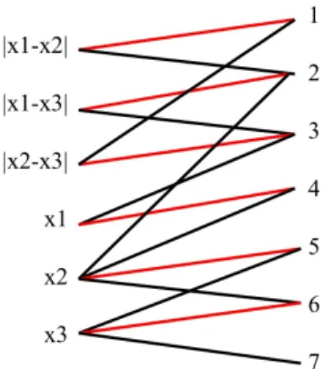
Therefore, if you select the wrong problem that is if you make the wrong abstraction, then you will miss the interesting part. On the other hand, if you select the right abstraction you could better understand the weakness of your CP model. For instance, the model for solving the Golomb Ruler clearly shows the weakness of the combination of symbolic (or counting) and arithmetic con-straints. Figure 4 shows a part of the solution of the alldiff constraint. We can clearly see that the combination of arithmetic and counting constraints is not really taken into account. It is not consistent to assign at the same time the variables x2 to 5, x3 to 6 and the absolute difference |x2− x3| to 3.
Unfortu-nately, we do not know any model which prevents such bad assignments. Thus, it is quite important to figure out which kind of combination is implied in your problem, that is to make the right abstraction.
Fig. 4: A current solution of a part of the alldiff constraint represented by red edges.
6
Conclusion
In this paper, we showed and detailed four common pitfalls when solving real world problems with CP. Our goal has been to recall some principles that are usually worthwhile in practice. First, we should avoid undivided models because the decomposition of a model into different subproblems, their resolution and
their recombination give often good results in practice. Second, even if we have clever strategies we should not forget that there is no ideal strategy and that we have to avoid some parts of the search quickly when there are not successful and apply principles like the random-restart mechanism. Then, we have to be careful with benchmarking and ensure that we will be able to extrapolate the results we obtained for some restricted version of the whole problem. At last, the identification of relevant subparts of the problem on which we should focus our attention is not an easy task and we should try to make the right abstraction.
References
1. C. Bessi`ere and J-C. R´egin. Enforcing arc consistency on global constraints by solving subproblems on the fly. In Proc. of CP’99, pages 103–117, Alexandria, VA, USA, 1999.
2. E. Falkenauer. A hybrid grouping genetic algorithm for bin packing. Journal of Heuristics, 2:5–30, 1996.
3. I. Gent. Heuristic solution of open bin packing problems. Journal of Heuristics, 3:299–304, 1998.
4. C. Gomes, B. Selman, N. Crato, and Henry Kautz. Heavy-tailed phenomena in sat-isfiability and constraint satisfaction problems. Journal of Automated Reasoning, 24(1/2):67–100, 2000.
5. R. Korf. An improved algorithm for optimal bin packing. In Proc. IJCAI-03, pages 1252–1258. 2003.
6. S. Martello and P. Toth. Knapsack Problems. John Wiley and Sons Inc, 1990. 7. J-F. Puget and J-C. R´egin. Solving the all interval problem. In CSP Lib. B. Hnich
and I. Miguel, 2001.
8. P. Schaus, J-C. R´egin, and P. Van Hentenryck. Scalable load balancing in nurse to patient assignment problems. In CP-AI-OR’09, pages 233–247, 2009.
9. A. Scholl, R. Klein, and C. J¨urgens. Bison: a fast hybrid procedure for exactly solv-ing the one-dimensional bin packsolv-ing problem. Computers & Operations Research, 24:627–645, 1997.
10. P. Van Hentenryck, L. Michel, L.Perron, and J-C. R´egin. Constraint programming in opl. In PPDP 99, International Conference on the Principles and Practice of Declarative Programming, pages 98–116, Paris, France, 1999.