Spatio-temporal intermittency in a 1D convective pattern: Theoretical model and experiments

HAL Id: cea-01374019

https://hal-cea.archives-ouvertes.fr/cea-01374019

Submitted on 29 Sep 2016

HAL is a multi-disciplinary open access

archive for the deposit and dissemination of

sci-entific research documents, whether they are

pub-lished or not. The documents may come from

teaching and research institutions in France or

abroad, or from public or private research centers.

L’archive ouverte pluridisciplinaire HAL, est

destinée au dépôt et à la diffusion de documents

scientifiques de niveau recherche, publiés ou non,

émanant des établissements d’enseignement et de

recherche français ou étrangers, des laboratoires

publics ou privés.

Spatio-temporal intermittency in a 1D convective

pattern: Theoretical model and experiments

F. Daviaud, J. Lega, P. Bergé, P. Coullet, M. Dubois

To cite this version:

F. Daviaud, J. Lega, P. Bergé, P. Coullet, M. Dubois. Spatio-temporal intermittency in a 1D convective

pattern: Theoretical model and experiments. Physica D: Nonlinear Phenomena, Elsevier, 1992, 55

(3-4), pp.287 - 308. �10.1016/0167-2789(92)90061-Q�. �cea-01374019�

Physica D 55 (1992) 287-308

North-Holland

PHYSICA

D

Spatio-temporal

intermittency in a 1D convective pattern:

theoretical model and experiments

F. Daviaud”, J. Legab,C, P. Berg&“, P. Coulletb, and M. Dubois”

“SPEC, CE Saclay, 91191 Gif-sur-Yvette cedex, France bINLN, Pare Valrose, B.P. 71, 06108 Nice Cedex 02, France

‘Department of Mathematics, University of Arizona, Bldg. #89, Tucson AZ 85721, USA

Received 10 April 1991

Revised manuscript received 3 October 1991 Accepted 16 October 1991

Communicated by A.C. Newell

We describe the occurrence of spatio-temporal intermittency in a one-dimensional convective system that first shows time-dependent patterns. We recall experimental results and propose a model based on the normal form description of a secondary Hopf bifurcation of a stationary periodic structure. Numerical simulations of this model show spatio-temporal intermittent behaviors, which we characterize briefly and compare to those given by the experiment.

1. Introduction

Rayleigh-BCnard experiments in both channel and annulus of small transverse aspect ratio [l-3] have shown transitions from laminar states toward spatio-temporal intermittency (ST11 [4]. The latter is described as a regime resulting from the competition between two metastable states, namely one fully turbulent and one completely laminar, and shows both spatially and temporally localized turbulent patches that appear in laminar domains. It has been observed in Kuramoto-Sivashinsky type equations [4] as well as in coupled maps [5], and widely analyzed [6]. So far, there is no clear understanding of the link between this kind of behavior and experimental results, but still they seem analogous. On the other hand, it has been early recognized [71 that normal forms or amplitude equations [S--101 give good descriptions of behaviors above first bifurcation thresholds, and, in some particular cases, they can be computed from “microscopic” equations [g-12]. The aim of this paper is to shed some light on a possible link between ST1 and experiments by giving a normal form description of the destabilization of a stationary periodic pattern, and by showing it may give rise to spatio-temporal intermittent behaviors. In the first section, we recall the main experimental results about ST1 in a convective pattern. Section 3 is devoted to the derivation of the model equations and their numerical simulations. Finally, we conclude with a short discussion of our results.

2. Summary of experimental results

In the following, we summarize experimental results on Rayleigh-BCnard convection in quasi one- dimensional (1D) systems. Detailed studies in both rectangular and annular cells have been reported elsewhere [2,3], and we shall focus on the dynamical regimes observed in an annulus (periodic boundary

288 F. Daviaud et al. / Spatio-temporal intermittency in a ID convective pattern

conditions). When increasing the Rayleigh number, the periodic stationary convective pattern first exhibits oscillatory regimes and propagation of spatial defects. Then, a transition to turbulence via spatio-temporal intermittency (ST11 occurs, which corresponds to a mixing of turbulent patches within laminar domains.

2.1. Experimental setup

We have studied Rayleigh-Btnard convection in an annular cell with a narrow gap. The latter was filled with silicon oil of Prandtl number 7. The vertical and horizontal walls were respectively made of Plexiglass and sapphire. The transverse aspect ratio was r, =,0.29, which is small enough to get a 1D geometry, and the circumferential aspect ratio was r, = 35. The temperature difference across the fluid layer was controlled at a precision of 0.01 K, by means of thermally regulated circulating water. After each temperature increase, dynamical equilibrium was awaited before making new data acquisition.

The convective structures were visualized by shadowgraphic imaging and their spatio-temporal evolution was recorded using a video camera. The image was digitized along a circle of 1024 pixels, giving a resolution of 2.5 pixels per wavelength (at the onset of STI, 40 wavelengths are present in the cell). The acquisition frequency was chosen between 1 image every 10 seconds and 10 images per second, in order to obtain information on the long-time evolution of the pattern, or on the exact dynamics of a turbulent event. Time series of several thousands of T,, were needed to perform statistics, where T, = 1 s is the basic period of the oscillating rolls.

2.2. Regimes observed

When Ra exceeds a critical value that depends on r,, perfect stationary patterns of rolls are observed; the rolls axis is then perpendicular to the longer side of the container (domain labeled by S in fig. 11. The number of convective rolls increases with the Rayleigh number, making the wavelength of the pattern much smaller than that observed in large containers. Moreover, a stable spatial inhomogeneity of the local wavelength is generally observed. This phenomenon, which is characterized by the coexistence of small and large cells, has also been observed in rectangular geometry, and a precise study is currently in progress [13]. However, near the onset of STI, the pattern is homogeneous, i.e. the distribution of wavelengths shows a sharp peak at A, = 0.44h,.

Above a given value of the control parameter E = Ra/Ra, - 1, the pattern becomes time dependent through the appearance of vacillations (domain D in fig. 1). The threshold value for this phenomenon depends on r, and on the present wavelength A,,. This regime, which has been described in detail in ref. [14], consists of oscillations of the hot and cold streams about their mean position (cf. fig. 2a1, cold and

T pre ST1 ST, ;_._.---j s

;___-2________;y

I I I L I I _* 200 400 6a 600 _E

Fig. 1. Schematic phase diagram of the convective state as a function of 8. S stands for a stationary pattern, D for dynamical regimes, ST1 for spatio-temporal intermittency and T for a complete disorganized and turbulent pattern.

F. Daviaud et al. / Spatio-temporal intermittency in a ID convective pattern 289

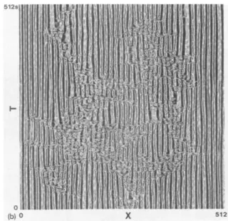
Fig. 2. Space-time evolution of the convective pattern obtained in the annular geometry. Spatial digitization is made over 1024 pixels. The light intensity is averaged over the nearest neighbors and plotted every other pixel, using a 256-level grey scale. (a) Vacillations; E = 400, (b) Pre-STI; E = 470, (c) STI; E = 540.

hot streams being out of phase. Near threshold (E = 200), the oscillations are monoperiodic, with a frequency f = 0.5 Hz. When E is increased further, a bi-periodic regime is observed. The oscillations strongly depend on the spatial structure of the pattern. More precisely, some parts of the cell oscillate and others do not, depending on the local wavelength. When the pattern is homogeneous, a quasi-perfect regime of oscillations can be observed, with the same frequency all over the cell. However, nodes of oscillations are present. In the monoperiodic regime, they correspond to points at rest, and are

290 F. Daoiaud et al. / Spatio-temporal intermittency in a ID conoective partern

associated with a standing wave for the amplitude of oscillations [14]. The bi-periodic regime corresponds to a periodic displacement of these nodes.

At a larger value of E, new events leading to a spatial symmetry breaking occur. They are characterized by the propagation of defects (or solitary waves, cf. refs. [2, 31). Then, above aa = 450, the interaction of these waves with the oscillators destabilizes the spatial structure, and turbulent patches are observed: the convective pattern enters the regime of STI. The pattern shows a mixture of organized laminar domains and incoherent turbulent domains (defined later), that are fluctuating in space and time.

At the onset of ST1 (cf. domain labeled by pre-ST1 in fig. 0, turbulent domains of small size seem to appear spontaneously. In the annular geometry, they are localized in space and time, and can propagate through the container with a constant velocity (0.8 h,,/T,, where A, is the mean wavelength). They may also locally break the spatial pattern of rolls. In the latter situation (see the spatio-temporal diagram of fig. 2b), a turbulent zone can spread by contaminating the next cells, or relax to a laminar state. Above a certain threshold (Ed = 480), turbulent domains never relax. We then have a regime of sustained intermittency (cf. domain labeled by ST1 in fig. 1). A typical spatio-temporal diagram is shown in fig. 2c. 2.3. Statistical measurements

As is well evidenced in fig. 2, turbulent patches have no spatial coherence, and a chaotic time evolution. On the contrary, laminar domains show a regular behavior in space and time; the periodicity of the pattern is preserved, and the shadowgraphic intensity at a given point is either stationary or periodic in time. A spatial criterion was taken to decide if locally the behavior is laminar or turbulent. If the local wavelength (i.e. the size of the cells) is such that A, - AA < A < A, + AA, where A, is the basic wavelength of the pattern and AA a tolerance factor, the behavior is said to be laminar; otherwise it is turbulent. Provided +A, < AA < $A,, AA has no major incidence on the statistics calculated from this binary reduction. Calculations performed (see ref. [3]) with a criterion based on the local temporal evolution gave similar results. In this case, the criterion was as follows: a cell i is said to be laminar if the shadowgraphic intensity Z(i, t) satisfies IZ(i, t + 1) - Z(i, t>l I 6, where 6 is a cutoff value properly chosen, i.e. such that no major change occurs in the results when 6 is varied.

A global characterization of the regime is given by the evolution of the turbulent fraction F,: F, is calculated as the averaged total length occupied by the turbulent cells, divided by the length of the container. The results show an increase of F, with E, but the transition looks imperfect (cf. fig. 3). This imperfection may be due to the annular geometry (for more detail and comparison with a rectangular cell, see ref. [3]), or come from the way measurements are made. Note that, in rectangular geometry, the dependence of F, on E gives a well-defined transition: Ft - (E - E,)~ with p = 0.3 [3] (the full curve in fig. 3 corresponds to a fit of the experimental points with @ = 0.3). Nevertheless, a power law decay is observed in the annulus at the threshold value E = Ed, for the distributions of the number N(L) of laminar domains of length L, and of the number N(r) of laminar domains lasting T. Above threshold, these distributions become exponential, defining characteristic length and time which diverge like (E - 520)-l’* (cf. fig. 4).

The experiments reveal the same qualitative route to turbulence via ST1 as in the numerical simulations of some partial differential equations like the Kuramoto-Sivashinsky equation

[hl,

coupled map lattices [5] and directed percolation [15], and most of the characteristic properties observed in the critical region around the threshold of ST1 are similar [2, 31. Nevertheless, there is no clear understand- ing of the link between experimental and numerical results. Here, a starting point is that the experiment described above shows that ST1 occurs after the appearance of temporal regimes. Besides, the perfect

F. Dauiaud et al. / Spatio-temporal intermittency in a ID conoective pattern 291

0 20 40 60 *o 480 500 520 54a 5w 5(10 800 820

L E

Fig. 4. (a) Histogram N(L) of laminar domains of length L, showing an exponential distribution at E = 530; (b) Square of the slope m, (computed from the exponential decay of the histograms of laminar domains) as a function of E.

vacillation pattern results from a Hopf bifurcation of the periodic 1D structure. Therefore, an approach to this problem consists in the study of the secondary Hopf bifurcation of a 1D pattern. In the next section, we show that spatio-temporal intermittent behaviors may be related to a phase instability of the order parameters associated with this secondary bifurcation.

3. Description through model equations

We consider a one-dimensional periodic pattern that undergoes a secondary Hopf bifurcation, thus leading to an oscillatory regime. We first characterize this bifurcation in order to get vacillations above threshold, and then describe the resulting dynamics by means of amplitude equations. Our intent is to show that, depending on external parameters, the latter equations model localized destruction of the vacillation pattern. More precisely, we shall show that a phase instability of the vacillation solution provides a mechanism for spatio-temporal intermittent-like behaviors in the system.

292 F. Daoiaud et al. /Spatio-temporal intermittency in a 1D conuectiue pattern

3.1. Description of vacillations

Vacillations result from the growth of an oscillatory mode that adds to the basic periodic structure, i.e. to stationary rolls. This mode is such that convective extrema display periodic oscillations for which maxima and minima are rr out-of-phase. This corresponds to oscillations of the second harmonic of a mode of same period as the basic pattern, but of opposite parity. Indeed, a mode of same period and same parity as the basic pattern would lead to beatings in the amplitude of convection, but not to periodic displacements of extrema, whereas a mode with same period and opposite parity would result in in-phase displacements of minima and extrema.

3.2. Model equations

We now analyze the Hopf bifurcation of a parity-invariant periodic pattern, for which the growing mode above threshold has a parity opposite to that of the initial pattern. In other words, we consider a

1D periodic pattern, described by U = U&X + cp), where U,(x) is an even function, and cp stands for the phase shift due to an arbitrary choice of the origin of space coordinates. This degree of freedom is reminiscent of the space translation invariance of the system before the first bifurcation, namely the one giving rise to the periodic pattern U,. We then assume that this pattern undergoes a Hopf bifurcation characterized by a temporal frequency o. Near this secondary bifurcation threshold, the quantity U can be written in the form [16, 171

U(x,t,cp,A) =Uo(x+‘p) +exp(i,t)A(x,t)5(x+cp) +c.c.+ . . . .

where C(x + cp) is the most unstable mode at threshold and is periodic in X, A is the complex amplitude associated with the Hopf bifurcation, c.c denotes complex conjugate, and the dots stand for higher order corrective terms. Since we want vacillations to occur above threshold, we assume that l has the same period as the basic pattern (which is in particular the case for a second harmonic), and an opposite parity. Thus, U depends on two quantities, namely cp and A, which are both assumed to vary slowly in space and time. The fact that cp, which can be thought of as the “phase” of U,, is now allowed to depend on space or time is crucial for the following, and simply comes from the fact that U, is marginal with respect to homogeneous “phase” perturbations, and therefore, its large scale “phase” variations should be taken into account in this description.

The dynamics of U is then ruled by that of 9 and A, which obey two coupled equations, whose form can be deduced by means of symmetry arguments. Namely, since U, is of given parity, i.e. since the system before the second bifurcation exhibits a reflection symmetry, then if U(x, t, cp, A) is a solution,

UC-x, t, -cp, -A) should also be an admissible solution. The negative sign in front of A in the latter expression is due to the odd parity of 5. Therefore, these equations should be invariant under the transformation

x-+ -x, (p-+ -cp and A+ -A.

Another symmetry comes from the invariance of the system under time translations before the second bifurcation. Then, if U(x, t, cp, A) is a solution, U(x, t + T, cp, A) should also be a solution, and therefore

F. Daviaud et al. / Spatio-temporal intermittency in a ID convective pattern 293

the evolution equations must be left invariant by the following transformation:

A -+A exp(i$),

where I,!J is an arbitrary real constant. Thus, the generic form of these two equations is [16, 171 aA

-=pA+(l+io)$-(l+i/3)]AI*A-(y+i~?)gA, _at

_(la>

(lb)

Here, p measures the distance from the Hopf bifurcation threshold, (Y and p express dispersion and nonlinear renormalization of the temporal frequency, y, 6, 5 and n are coupling coefficients, and K is the diffusion coefficient of the phase cp. Some prefactors have been set to one after scaling the space coordinate and A. The other coefficients are of order 1 a priori. The first part of eq. (la) is the classical Ginzburg-Landau equation associated with a Hopf bifurcation [18]. The coupling with the phase of the basic pattern U, simply means that the growth rate of A (cf. the term proportional to -y> and its temporal frequency (term in S) are modified if the basic pattern is compressed or streched (i.e. if its phase gradient @/ax is negative or positive). The coupling terms in eq. (lb) mean that the phase is sensitive to amplitude (term in 5) and phase (term in 7) variations of A. Let us mention that we would have obtained the same equations if 5 had had the same parity as the basic pattern, or if its period had been twice as big as that of the initial structure [16].

Above equations possess a “laminar state” (LS), given by

A=A,=aexp(-iP@+i&), (p=‘po,

whose stability is investigated below. Here, $. and (p. are arbitrary constants. Notice that this solution corresponds to vacillations of the periodic pattern, according to the description of U we gave above. For LS, eq. (la) is uncoupled to eq. (lb), i.e. A obeys the complex Ginzburg-Landau equation. But, if 1 + c+? < 0, this latter equation is known to produce phase turbulence [18, 191, and eventually leads to the destruction of the solution A,, through the appearance of zeroes of A. Hence, here is a possible way for spatio-temporal intermittent behaviors to occur in the system, and therefore, our guideline for the followmg will be to choose the parameters such that the laminar solution

phase perturbations, and see whether the coupling with the phase cp of the instability or dampens it.

is unstable with respect to basic pattern enhances this

3.3. Linear stability of the laminar state - conditions for phase instability

Since LS is marginal with respect to homogeneous phase perturbations of 50 and of the phase of A denoted I/J, and since amplitude perturbations of A are damped (see appendix), the dynamics of the system about LS can be reduced, at least when LS is stable, to two coupled phase equations [18] for cp and I/J, Their derivation, together with the linear stability analysis of LS, is carried out in the appendix.

294 F. Daviaud et al. /Spatio-temporal intermittency in a ID conuectice pattern

They read

(2b)

These equations reflect the symmetries of eqs. (1). Namely, they are invariant under the transformation

Moreover, without coupling, i.e. with y = 0 and 6 = 0, eq. (2a) is the well-known phase equation [18] or Kuramoto-Sivashinsky [20, 211 equation associated with the complex Ginzburg-Landau equation.

The two phase eigenvalues, expanded as a power series of any fourier mode k, read (see appendix)

h=h(k)= +/i,k-;[l+@+K+y(f+e)]k2+...,

where A: = 277&y - 6). Therefore, if c = np(py - 6) < 0, A, is pure imaginary and LS is stable as soon as D = 1 + CY~ + K + y(& - 5) is positive. Hence, the coupling between the complex amplitude A and the phase cp of the basic pattern may delay the occurrence of phase instability for A, since 1 + (YP may be negative whereas D is positive. But, when D becomes negative, LS is phase unstable, and may then display STI. Therefore, our ST1 control parameter will be D. When c is positive, LS is always unstable, whatever D may be, and here again, ST1 may occur.

3.4. Numerics

Before describing the dynamics of eqs. (1) when LS is phase unstable, let us first consider some numerical aspects of the problem. Since only spatial derivatives of cp are relevant, it is more convenient for the numerics to deal with r = +/ax instead of cp, and therefore, we consider the following equations, which are deduced from eqs. (2):

aA

-=~A+(l+iru)$-(l+i/?)IA~2A-(y+i8)E4,

at

(3b)

As an initial condition, we take the laminar solution LS, slightly randomly perturbed. The numerical

simulations have been performed on a CRAY-YMP, using a pseudo-spectral code with periodic

boundary conditions. The number of collocation points was 1000, and the box length was 300 units of length. Now, we need to overcome two problems: how to cope with the nucleations or annihilations of cells in the basic pattern, and how to distinguish laminar cells from turbulent ones.

Since we only take into account the phase of the basic pattern, these equations cannot describe the existence of nucleations of new pairs of cells, or their annihilation. Nevertheless, when the phase gradients of cp become high enough, two cells should annihilate, or a new pair should be created. The occurrence of one of these two events depends on the sign of the phase gradient, i.e. if the pattern is

F. Dauiaud et al. /Spatio-temporal intermittency in a ID convective pattern 295

compressed or streched. In order to implement these nucleation events in our model, we introduce a cutoff value r, above which r is set to zero. This stands for the fact that when phase gradients (r) of cp are too high, annihilations or nucleations occur in order to relax the phase, and therefore r gets smaller. The after-cutoff discontinuity in r will be smoothed by the numerics, and this ad hoc perturbation is assumed to describe the one which is introduced by the nucleation or annihilation of cells in the basic pattern. So, for each time step, and at each point,

if T(x) >TO then T(x) =O.

We have chosen r, = 1 and checked that such perturbations do not bring aliasing into the numerics. The second stage is to choose a criterion to separate laminar cells from turbulent ones. Like in the experiment, we define “turbulent” as “which departs from laminar”, and since LS is characterized by IA I = 6 and (aA/at > + iPpA = 0, our criterion will be as follows:

if laA/at + @pAI

I4 < s then the cell is laminar,

if laA/at + @pAI

IAI r s then the cell is turbulent.

(da)

In other words, a cell is said to be “turbulent” if A is small or if the local behavior is no longer periodic at the right frequency. In the simulations, we have chosen s = 0.65, and checked the results are not sensitive to the very value of this threshold. Note that, given the fact that amplitude equations cannot describe the periodic pattern at the scale of its period, this criterion is close to the one used in the experiment. Indeed, since A is the order parameter associated with the Hopf bifurcation, a small value of A corresponds to a spatial destruction of vacillations (therefore a cell should be turbulent if l/ IA I is large), whereas a change in its temporal frequency means temporal irregularity in the oscillations of the pattern (whence the use of IaA/at + i/?pAl as a second criterion). The conjunction of the two in (4) allows us to define a turbulent patch as showing irregularity either in time or in space, which is the definition used in the experiment.

3.5. Occurrence of spatio-temporal intermittent behaviors

We have seen that there are two ways of destabilizing the laminar solution LS, either by choosing D < 0 or by taking c > 0. We first consider these two situations separately.

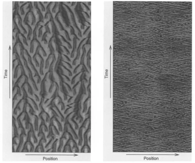
When c < 0 and D < 0, the instability of LS is analogous to the Benjamin-Feir [lo] instability of the complex Ginzburg-Landau (CGL) equation, except that D is now given by D = 1 + CY@ + K + -y(/3~~ - 51, whereas it is 1 + a@ for CGL alone. This instability gives rise to the appearance of dips in the amplitude of A, that travel with a constant velocity, at least close to threshold. Fig. 5 shows a spatio-temporal diagram of the system when D = -0.3. Black spots correspond to “turbulent” cells according to criterion (4b), and white regions are laminar domains, that satisfy (4a). Black or “turbulent” lines correspond to above-mentioned traveling dips, which are reminiscent of the traveling hole solutions to CGL described by Bekki and Nozaki [22]. The structure of one of these objects is detailed in fig. 6. A rapid variation in the phase of A occurs at the center of the depression and, depending on the asymptotic wavevectors, the dip propagates to the right or to the left. These two kinds of propagations correspond to lines slanted to the right or to the left on the spatio-temporal diagram of fig. 5. The

296 F. Daviaud et al. /Spatio-temporal intermittency in a ID convective pattern

Fig. 5. Numerical simulation of eqs. 3, with p = 1, a = 1, p = -1.2, y = 0.5, 6 = 0.3, .( = 1, 77 = 1 and K = 1. The evolution of the pattern is represented here during 1300 units of time. The entire box is shown, which corresponds <to 300 units of length in the x direction. Laminar regions are white, turbulent domains are black, according to (4).

Fig. 6. Amplitude (a) and phase (b) of one of the traveling dips in fig. 5. The value of IA 1 at the center of the dip and the amplitude of the “phase jump” change as the dips propagates.

F. Daviaud et al. / Spatio-temporal intermittency in a ID convective pattern 297

Fig. 7. Same as fig. 5, but with p = - 2.5.

Fig. 8. Spatio-temporal diagram for the amplitude of A. Minima arc in dark and maxima correspond to lighter regions. Only one half of the box is shown, and during a period of 1000 units of time. The parameters are the same as in fig. 7.

traveling hole solution described in [22] is characterized by the fact that its velocity is related to the phase shift between the asymptotic waves. Because of the phase instability, the dips we observe always evolve in time and we cannot make accurate measurements of their asymptotic wave numbers. However, it is likely that, close to the phase instability threshold, these wave numbers are related to the wave vector k,,, whose growth rate is maximum. This could explain why the velocity of the dips is almost constant near threshold. Indeed, the wavenumbers on both sides of the dips should be close to kk,, and, as a consequence, their velocities would be nearly equal in absolute value. At this stage, we cannot give any quantitative check of this possible explanation. When IDI is increased further, the density of dips gets higher and their velocity is not as well defined as before. Fig. 7 shows a spatio-temporal diagram analogous to that of fig. 5, but for D = -2.25. For this picture, the mean value of r is about 0.12. Thus, the binary picture defined by (4) is less meaningful than before, since the amplitude of A and its temporal frequency are modified by the phase gradients (r) of the basic pattern. Fig. 8 shows a

298 F. Daviaud et al. /Spatio-temporal intermittency in a ID convective pattern

Fig. 9. Same as fig. 8, but with p = 1, (Y = 1, p = -0.8, y = 0.5, 6 = - 0.5, 5 = 1, 77 = 1 and K = 1.

Fig. 10. Same as fig. 8, but with fi = 1, (Y = 1, p = - 1. y=0.5,6=-0.9,[=1,~~=1and~=l.

spatio-temporal diagram for the amplitude of A for the same value of D. Finally, let us mention that the dynamics described here is similar to that which is observed for CGL alone when its homogeneous solution is Benjamin-Feir unstable [231.

When c > 0 and D > 0, the instability is stronger and results in persistent localized destruction of the pattern, that shows less propagation and few branching. The number of “nucleations” (i.e. the number of times r gets higher than the cutoff value To) is bigger than before. In these regimes, the binary picture defined by (4) is not very informative, and we only show spatio-temporal diagrams for the amplitude of A. Fig. 9 is such a diagram for D = 0.3 and c = 0.1, where we see that the main feature is the existence of localized amplitude variations. When c is increased further, the number of “nucleations” gets higher again, and the mean value of r is no longer close to zero.

Finally, fig. 10 shows the behavior of the amplitude of A for D = -0.15 and c = 0.35 (i.e. both conditions for instability are satisfied). The pattern is now strongly destroyed and few branching phenomena occur. Here again, the number of “nucleations” is high and the man value of r (?; = 0.23) is

F. Daviaud et al. / Spatio-temporal intermittency in a ID convective pattern 299

not close to zero. Because of the increasing number of “nucleations” in the basic pattern, we cannot push further the analysis of this regime since the description with amplitude equations would no longer be valid.

3.4. Measurements

We focus on the regime where D < 0 and c < 0, which is characterized by the propagation of dips in the amplitude of A. The simulations have been performed with p < 0 variable and p = 1, (Y = 1, y = 0.5, 6 = 0.3, ,$ = 1, 77 = 1 and K = 1. Then c is always negative, and D is given by D = 1.5(1 + p). For each value of p, we compute the distribution of lengths of turbulent and laminar cells as well as their mean values, together with the turbulent fraction F,, measured in the ST1 regime, and defined as

F, = number of turbulent cells _{number of cells} > f’

where ( . >, means average over time. Since LS is stable when D > 0, Ft is zero when p > - 1. The turbulent fraction increases as lpl gets larger, and its behavior is given in fig. 11. The near-threshold behavior resembles ST1 in the sense that Ft scales like a power of the control parameter, though the exponent here is close to one. Besides, the picture we get is close to that which is got experimentally. However, there is no imperfect transition here, since the ST1 threshold is quite definite.

The mean length of turbulent regions increases with IDI a -(l + p). More interesting is the mean length of laminar regions, which decreases as IDI a -(l + /3) increases, i.e. as ST1 goes stronger. Since the real parts of the phase eigenvalues (see appendix) are given by

Re(h) = h,k2 + h,k4, where A, > 0 and A, < 0, the larger excited mode is

and therefore, laminar regions of length I such that 21r/l> k,,, should remain laminar, since they are now stable. Close to threshold, A4 is finite and k,,, scales like 6 = d-. For the particular

. 0.8 - _. 0.6 - . 0.4 - . . 0.2 - . . 0 . . . . . . . ..I.... -1 0 1 2 -U+B

Fig. 11. Behavior of the turbulent fraction F, as a function of the order parameter -Cl + p) a ID I. Measurements have been made from samples consisting of 3000 consecutive states (distant from each other by one unit of time) of the 1D system, and for various values of /I?. Other parameters were kept constant (see text).

F. Daoiaud et al. / Spatio-temporal intertnittency in a ID conuectiuepattern . . . l . 0 (....I’..‘I’,“I”,‘I’,“( 0 0.5 1 1.5 2 2.5 (_l+)-“*

Fig. 12. Behavior of the mean length of laminar domains, as a function of [ - (1 + p)]-‘/2.

01, t

0 20 40 60 80 100 length of laminar domains

arbitrary units (box length = 300)

Fig. 13. Typical behavior of the distribution of laminar lengths, computed from a sample of 3000 consecutive states (distant from each other by one unit of time) of the 1D system. Here p = 1, (Y = 1, p = - 1.6, y = 0.5, 8 = 0.3, 5 = 1, n=land~=l.

parameter values chosen here, we have D = 1.5(1 + p) i.e. & a [ - (1 + p)]‘/*. Thus, the maximum length of laminar domains I,,, should be proportional to [ - Cl+ @)I-“*. In fig. 12, we have plotted the behavior of the mean length of laminar domains as a function of [-Cl + /?>I-iI*. It is linear near threshold (large values of [-Cl + p)]-1/2>. Hence, we have the following picture: laminar regions larger than I,,, are phase unstable, which give rise to patches of “turbulent” cells. Their appearance results in shortened laminar regions, which are now stable since they are too short for phase instability to develop. If laminar regions become too large, new turbulent patches appear, and the system goes, in space and in time, from laminar to “turbulent states”, in an intermittent way.

Finally, we have computed the distributions of laminar and turbulent lengths. A typical distribution behavior is given in fig. 13. We have always observed an exponential decay, even for values of D close to the threshold value D = 0. However, we cannot go too close to D = 0 since the time then required for ST1 to develop gets too long. Nevertheless, fig. 14 shows the behavior as a function of D of the inverse of the square of the characteristic length associated with the exponential decay of these distributions. This

. l

0 .-._,‘...,....,....,.... Fig. 14. Inverse of the square of the characteristic length of

0 0.5 1 1.5 2 2.5 the distribution of laminar lengths, as a function of -(l + p) -(l+P) a ID I. (Box length = 300.)

F. Daviaud et al. / Spatio-temporal intermittency in a ID convective pattern 301

characteristic length gets very large for D small, which leaves open the possibility of an algebraic decay at threshold. But we cannot give a definite answer to this question since we do not have points close enough to threshold (this would require boxes of increasing length and much longer computations), and also because the measure of the characteristic length from the distributions is not highly accurate.

4. Conclusion

We have shown that the two coupled equations describing a secondary Hopf bifurcation of a 1D periodic pattern can display spatio-temporal intermittent behaviors. The basic idea is that a phase instability of the order parameters associated with the secondary bifurcation can create localized patches of “turbulent” domains. The latter appear randomly in space, and their lifetime is also arbitrary. This coexistence of laminar and turbulent patterns is characteristic of spatio-temporal intermittency. How- ever, this picture does not correspond to a competition between two “metastable” states, one turbulent and one laminar, since the laminar state is definitively unstable when D < 0 or c > 0, at least in a box whose length is large enough. Here, the term spatio-temporal intermittency denotes an alternance in space and time of laminar and “turbulent” behaviors, and is not as specific as it was originally [4, 61.

The mechanism we propose qualitatively reproduces the experimental observations. For instance, for

D > 0 and c < 0, the system features turbulent cells that propagate through the system at a constant velocity near threshold. This is reminiscent of the propagation of turbulent patches observed experimen- tally in the pre-ST1 regime (cf. section 2.2). Fully developed ST1 seems to be qualitatively well described by the regime corresponding to c > 0 and D < 0. Finally, the evolution of the turbulent fraction and of the characteristic length are similar (cf. figs. 3 and 11, figs. 4, 13, and 14). Thus, a phase instability associated with a secondary Hopf bifurcation of the convective pattern could be a possible explanation of ST1 in the Rayleigh-BCnard experiment.

Nevertheless, many questions are still open. For instance, we have assumed a Hopf bifurcation towards idealized vacillations. But the existence of regimes without oscillations, or the presence of a standing wave for the amplitude of oscillations have not been considered. This latter situation might though be described by assuming that the Hopf bifurcation occurs for a wavevector k which is non-commensurable with that of the basic pattern. This would then lead to three coupled equations (see ref. [16]), that are likely to give behaviors analogous to those of the two equations we have considered. More importantly, we have not proved that a phase instability does occur in the experiment, even though this work concludes it is likely. For these reasons, the next stage of this study is to start from the hydrodynamic equations (which turn out to be tractable since we have a 1D problem), and numerically follow the convective solution till its secondary bifurcation occurs. This should then allow a complete characteriza- tion of the secondary bifurcation for this experiment, and determine the signs of c and D for the envelope equations. Experimental and numerical work in this direction is in progress.

Acknowledgements

We are grateful to H. Chat&, S. Fauve, P. Manneville, T. Passot and Y. Pomeau for fruitful discussions. We acknowledge the EEC twinning project Spatio-temporal chaos in extended systems (No. SCl-0035-C (CD)) for financial support. Two of us (P.C. and J.L.) wish to acknowledge the Arizona Center for Mathematical Sciences (ACMS) for support. ACMS is sponsored by AFOSR contract FQ8671-9000589

302 F. Daviaud et al. / Spatio-temporal intermittency in a ID convectiue pattern

(AFOSR-90-0021) with the University Research Initiative Program at the University of Arizona. Finally, we thank the Pittsburgh Supercomputing Center where the numerical simulations have been performed, under grant number DMS900005P.

Appendix

In this appendix, we perform the linear stability analysis of the laminar state (LS) given by

A=A,=fiexp(-iPpLt+i$,), cp=‘pO,

which is a solution to eqs. (1):

Writing

we get for the linearized system about LS:

aa

at=

-p(l+ip)(u+Z)+(l+iu)$-(v+ia)&+!j$. aa

at= -I*(l-iP)(a+Z)+(l-ia)$-(T-i~)fi~7

and the eigenvalues A associated with the Fourier mode k are solutions to

-p(l+ip)-(1+icu)k2-A _{-4l+ iP)} -ik( y + iS)fi

o=

_{--c~(l -}

_iP) -p(l-ip)-(l-ia)k2-A -ik(y-ii3)fi

ik&&--Gk ik56+qak -tck2 -A

-2p-(l+ia)k2-A -2~ - (1 - ia)k2 - A -2ikya

= _{-4l- iP)} -p(l-i/3)-(l-icu)k2-A -ik(y-iG)&

ik56 - rlfik ik5fi+q&k -tck2 - A

-2~ - (1-t iCu)k2 -A 2iak2 -2ikyfi

= _{-lu(l- iP)} -(1-ia)k2-A -ik(y-i6)a

(la)

(lb)

F. Daviaud et al. /Spatio-temporal intermittency in a ID conraective pattern 303

i.e.,

[-2~-(l+icy)k2-A][h2+Ak2(1- icu + K) + K( 1 - ia) k4 + 2iqpk2( y - is)]

+ ~(1 - ip)( -2iaKk4 - 2i(uAk2 + 4iyqpk2)

+k~(i,$-n)[2~~(y-ii6)fik~-2ikyfiA-2iyfi(l-icu)k’] =O.

Expanding A as a series of powers of k,

A=Ao+kA,+k2A2+...,

we get: At order 0:

A;( -2~ - A,,) = 0,

that is, A, = - 2~ or A,, = 0. The existence of a double zero-eigenvalue corresponds to the fact that LS is marginal with respect to homogeneous phase perturbations on both cp and the phase I/J of A.

At order 1

-A,,A,(~P + 3A,,) = 0,

which is always satisfied if A,, = 0, and gives A, = 0 if A,, = - 2~. At order 2

0 = ( - 2~ - A,) [A: + 2A,,A, + A,,( 1 - ia + K) + 2ir/p( y - is)] - 2A& -(1+ia+A2)A~+~(1-i~)(-2i~A,,+4i~~~)-(i~-~)~(2i~~AO),

which gives

A:= -2p77(6-/3py) if A,=0 and

A,= -(l-cup) +y(pn -5) if A,= -2~.

At order 3

-A,Ai=O, i.e. A,=O,if A,= -2~

and

-2j~[2ArA~+A,(l -ICY +K)] -A,[A: +2irl~(y-i6)] +~(l -iP)(-2iaA1)

304 F. Daviaud et al. / Spatio-temporal intermittency in a ID convective pattern

which yields

A,= -+[l+C@+K+y(/3~--)] ifh”=o.

Thus, the three eigenvalues associated with the linearized problem about LS read

AR=-21L-[(1-(YP)-Y(P?7-~)lk2+~(k4),

A,= kA,k-;[l+ap+K+y(Pq-[)]k2+8(k3),

where Ai = 2~77(py - 6). The first eigenvalue, which is associated with amplitude perturbations of A, is negative for small k, and therefore amplitude perturbations are damped. The two other eigenvalues correspond to phase perturbations of cp or $. They vanish for homogeneous perturbations (k = 0) and may become positive if c = p~(py - 6) > 0 or D = 1-t a/3 + K + y(/3q - 5) < 0. When c < 0 and D < 0, it is often useful to push further the expansion of A + to see how it decays for larger k. Since the computation is somehow cumbersome, we will only show that A, is pure imaginary (when c < 0) and A, is real.

At order 4, we get, assuming A, = 0

-2~[A~+2A,A3+A2(1 -iia+~) +~(l -icy)] -A,[2A,A~+Al(l -ia+K)]

-(l+i(~+A~)[A~+2i~~(y-i6)] +~(1-$)[-2i(~K-2ic-uA~]

+ a( it - 7) [2cu( y - iS)fi - 2iy&A, - 2iyfi( I- ia)] = 0, which yields

2A,A, =

h2[

A, + 277( 6 -

Pr)] +

77(6 -

h’)(l + K) -

K-Y?7P+ff(Y77Y--LYPK+5~~+ty.

The right hand side is real, and since A, is pure imaginary, A, is also pure imaginary; moreover, A, and A, have same sign.

At order 5, the equation for A, reads

-2~[2AzA3+2A,A4+Aj(1-icu+~)] -A,[A~+2AlA3+AZ(1--ia+~)+~(1-i~)]

-(1+icu+h2)[2A1h2+A,(l-~(Y+K)] -A,[A:+2ipv(y-i6)]

+ p( 1 - ip)( -2iaA,) + F(it - v)( -2iyA,) = 0, which gives

2PA4 = +[ 776 - npy - rs] - 3A’, - 4A, - 2~h, - 2K - (1 + a’).

1

Here again, the RHS is real and therefore, A, is real. Thus, when c < 0, the two phase eigenvalues are given by

F. Daviaud et al. /Spatio-temporal intermittency in a ID convective pattern 305

Close to IST threshold, A, = 0, and

Since A, and A, have same sign, A, is negative, as soon as (A,/A,Xv6 - qPy - ~5) is not too large. Then, the real part of A + behaves like

Re(A,) = lA,lk2- IA,lk4+@(kh).

Since amplitude perturbations are damped (cf. A, < O), the dynamics about LS can be described [18] by that of the two phases cp and $, when LS is stable. In the following, we derive these phase equations up to order two in space derivatives. We look for a solution to eqs. (1) in the form

A=(fi+

EU, + E2U2 + . ..)exp[-i&+i$]

where E is a small parameter, and we assume that cp, IJ and the ui’s vary slowly in space and time. Therefore, the space and time derivatives are transformed as follows:

a a a a

- _ax + - _ax +E- _ax, +e2- + . ..) a a a a

3x2

- _at + - _at fez- _azy +e2- _aT2 + . . . .

We plug this into eqs. (1) and identify at each order in E. Order 0 is satisfied since we look for solutions about LS, which is a solution to eqs. (1).

At order 1, we get

$[c+exp(-iPLLr+i$)J

+$-[fiew(-iPW+iQ)]

= pul exp( - i@Ft + i$)

+(l+ia) 2&&[fiexp(-iPpt+i$)] +$[u,exp(-@j~t+i$)])

i

-(I + ip)[3pu, exp( -iPp.t + i$)] - (Y + ia) 6% exp( -iN + i@) 7

( 1

aP

-=

aT1

-2q1m

[(

a[\/;rexp(-iPpt+i$)]

ax1

+&[u,exp(-i&t+i$)])&exp($~t-ig)].

Since the phases cp and $ as well as the ui’s are assumed constant at fast space and time scales, we get

3 =(Br-s)& 1 acp a* - = -2yji4, aT* Y acp -- u1 = - 2fi ax, f (**I) (A.9 (A-3)

306 F. Dauiaud et al. /Spatio-temporal intermittency in a ID convective pattern

At order 2, we have

&[fiexp(-ippt+i$)] + &[u,exp(--iPj..d+i$)l +

$iheW(_iPW+i@)l

1

= pu, exp( -i&t + i+)

+(l+ia) $[

i

u*exp( -iPpt+ i$)] +

2$&[u,exP(-iSPt+i+)l

I

+2$&[&exp(-iP++i$)] + &[fiexp(-iPpt+i+)]

1 i

- (1 + ij?) (36 u: + ~PL+) exp( - iP@ + i(cr)

-(r+ia) JLT$+ )

( 2.4,s exp( -i&t + is),

8 =4264&j

-2qIm U, &[J;I.exp(-iPpt+i$)] +&[u,exp(-iPpt+ill)])exp(+iPiLr-iti)

[ ( 1

+&exp(ippt-i$)

(

&[&eq(-iPILt+i$)]

+ &[U,ew(-iPpt+ilL)]

iI

j$

+KaX:'

which gives

F. Daviaud et al. / Spatio-temporal intermittency in a ID convective pattern 307

which yield, using (A.3) and (A.2):

Finally, writing

we have

References

[l] P. Bergi, Nucl. Phys. B (Proc. Suppl.) 2 (1987) 247; S. Ciliberto and P. Bigazzi, Phys. Rev. Lett. 60 (1988) 286. [2] F. Daviaud, M. Dubois and P. Berg&, Europhys. Lett. 9 (1989) 441. [3] F. Daviaud, M. Bonetti and M. Dubois, Phys. Rev. A 42 (1990) 3388. [4] H. Chatt and P. Manneville, Phys. Rev. Lett. 58 (1987) 112;

U. Frisch, Z.S. She and 0. Thual, J. Fluid Mech. 168 (1986) 221; B. Micolaenko, Nucl. Phys. B (Proc. Suppl.) 2 (1987) 453;

H. Chat& and B. Nicolaenko, in: New trends in nonlinear dynamics and pattern forming phenomena: the geometry of

non-equilibrium, eds. P. Coullet and P. Huerre (Plenum, New York, 1990). (51 K. Kaneko, Prog. Theor. Phys. 74 (1985) 1033;

H. Chat& and P. Manneville, Physica D 32 (1988) 409; H. ChatC and P. Manneville, Europhys. Lett. 6 (1988) 591; H. ChatC and P. Manneville, J. Stat. Phys. 56 (1989) 357; K. Kaneko, Physica D 34 (1989) 1.

[6] For a review, see H. Chat&, Ph.D. Thesis, Paris, 1989.

[7] C. Normand, Y. Pomeau and M. Velarde, Rev. Mod. Phys. 49 (1977) 581;

J.E. Wesfreid, Y. Pomeau, M. Dubois, C. Normand and P. Berg& J. Phys. (Paris) 39 (1978) 725. [8] L.A. Segel, J. Fluid Mech. 38 (1969) 203.

308 F. Dauiaud et al. / Spatio-temporal itiermittency in a ID convective pattern

[lo] A.C. Newell, Lect. Appl. Math. 15 (Am. Math. Sot., Providence, 1974).

[ill E.D. Siggia and A. Zippelius, Phys. Rev. Lett. 47 (1981) 835; Phys. Rev. A 24 (1981) 1036.

[12] K. Kaiser, W. Pesch and E. Bodenschatz, Mean flow effects in the electro-hydrodynamic convection in nematic liquid crystals, preprint (1990).

I131 J. Hegseth, J.M. Vince, M. Dubois and P. Berg& submitted to Europhys. Lett.

[14] M. Dubois, R. Dasilva, F. Daviaud, P. Berg& and A. Petrov, Europhys. Lett. 8 (1989) 135. 1151 Y. Pomeau, Physica D 23 (1986) 3.

1161 P. Coullet and G. Iooss, Phys. Rev. Lett. 64 (1990) 866. [17] J. Lega, Eur. J. Mech. B/Fluids 10 (1991) 145.

[18] Y. Kuramoto, Suppl. Prog. Theor. Phys. 64 (19781 346; Chemical Oscillations, Waves and turbulence, Springer Series in Synergetics, ed. H. Haken (Springer, Berlin 19841.

[19] Y. Pomeau and P. Manneville, J. Phys. Lett. 40 (1979) 609. [20] Y. Kuramoto and T. Tsuzuki, Prog. Theor. Phys. 55 (1976) 356. I211 G.I. Sivashinsky, Acta Astronaut. 4 (1977) 1177.

[22] N. Bekki and K. Nozaki, Phys. Lett. A 110 (1985) 133. 1231 L. Gil, Nonlinearity 4 (1991) 1213.