How does Party Fractionalization convey Preferences for Redistribution in Parliamentary Democracies ?

HAL Id: halshs-00348878

https://halshs.archives-ouvertes.fr/halshs-00348878

Submitted on 22 Dec 2008

HAL is a multi-disciplinary open access archive for the deposit and dissemination of sci-entific research documents, whether they are pub-lished or not. The documents may come from teaching and research institutions in France or

L’archive ouverte pluridisciplinaire HAL, est destinée au dépôt et à la diffusion de documents scientifiques de niveau recherche, publiés ou non, émanant des établissements d’enseignement et de recherche français ou étrangers, des laboratoires

How does Party Fractionalization convey Preferences for

Redistribution in Parliamentary Democracies ?

Bruno Amable, Donatella Gatti, Elvire Guillaud

To cite this version:

Bruno Amable, Donatella Gatti, Elvire Guillaud. How does Party Fractionalization convey Preferences for Redistribution in Parliamentary Democracies ?. 2008. �halshs-00348878�

Documents de Travail du

Centre d’Economie de la Sorbonne

Maison des Sciences Économiques, 106-112 boulevard de L'Hôpital, 75647 Paris Cedex 13

How does Party Fractionalization convey Preferences for Redistribution in Parliamentary Democracies ?

Bruno AMABLE, DonatellaGATTI, ElvireGUILLAUD

How does Party Fractionalization convey Preferences for

Redistribution in Parliamentary Democracies?

Bruno Amable, Donatella Gatti and Elvire Guillaud Abstract

In this paper, we highlight the link between the political demand and social policy outcome while taking into account the design of the party system. The political demand is measured by individual preferences and the design of the party system is defined as the extent of party fractionalization. This is, to our knowledge, the first attempt in the literature to empirically link the political demand and the policy outcome with the help of a direct measure of preferences. Moreover, we account for an additional channel, so far neglected in the literature: The composition effect of the demand. Indeed, the heterogeneity of the demand within countries, more than the level of the demand itself, is shown to have a positive impact on welfare state generosity. This impact increases with the degree of fractionalization of the party system. We run regressions on a sample of 18 OECD countries over 23 years, carefully dealing with the issues raised by the use of time-series cross-section data.

Keywords: Political Demand, Party Fractionalization, Redistribution, Time-Series-Cross-Section Data JEL Code: D78, H10, H53, C33

La fragmentation des partis affecte-t-elle les préférences en matière de redistribution dans les démocraties parlementaires ?

Résumé

Dans cet article, nous mettons en lumière le lien entre la demande politique et la politique sociale, et la manière dont ce lien est affecté par la concurrence politique. La demande politique est mesurée par les préférences individuelles, et le système de partis est caractérisé par son degré de fragmentation. C’est à notre connaissance la première tentative dans la littérature de lier empiriquement la demande politique et la politique économique, avec l’aide d’une mesure directe des préférences. De plus, nous analysons un canal supplémentaire, jusqu’ici négligé dans la littérature : l’effet de composition de la demande. En effet, nous montrons que l’hétérogénéité de la demande au sein des pays, plus que le niveau de la demande en soi, a un impact positif sur la générosité de l’Etat social. Cet impact est croissant avec le degré de fragmentation du système de partis. Nous menons des régressions sur un échantillon de 18 pays de l’OCDE et 23 années, en portant une attention particulière aux difficultés engendrées par l’utilisation de données de panel.

Mots-clefs : Demande Politique, Fragmentation des Partis, Redistribution, Données de Panel Classification JEL : D78, H10, H53, C33

How does Party Fractionalization convey

Preferences for Redistribution in

Parliamentary Democracies?

Bruno Amable, Donatella Gatti

and Elvire Guillaud

November 6, 2008

Abstract

In this paper, we highlight the link between the political demand and social policy outcome while taking into account the design of the party system. The political demand is measured by individual pref-erences and the design of the party system is de…ned as the extent of party fractionalization. This is, to our knowledge, the …rst attempt in the literature to empirically link the political demand and the policy outcome with the help of a direct measure of preferences. Moreover, we account for an additional channel, so far neglected in the literature: The composition e¤ect of the demand. Indeed, the heterogeneity of the demand within countries, more than the level of the demand itself, is shown to have a positive impact on welfare state generosity. This impact increases with the degree of fractionalization of the party sys-tem. We run regressions on a sample of 18 OECD countries over 23 years, carefully dealing with the issues raised by the use of time-series cross-section data.

Keywords: Political Demand, Party Fractionalization, Redistribu-tion, Time-Series-Cross-Section Data

JEL Code: D78, H10, H53, C33

Université Paris I Panthéon-Sorbonne, CES and CEPREMAP

y_{Université Paris Nord, PSE and IZA}

Contents

4.2 Interaction Term and Marginal E¤ect . . . 15

4.3 Basic Results . . . 16

5 Criticisms and Further Results 17 5.1 Introducing Fixed E¤ects . . . 17

5.1.1 Model Speci…cation with Fixed E¤ects . . . 17

5.1.2 Heteroskedasticity and Spatial Correlation . . . 18

5.1.3 Results of Fixed E¤ects Regressions . . . 19

5.2 Coping with Time-invariant Variables and Fixed E¤ects . . . 20

5.2.1 Fixed E¤ects Vector Decomposition Procedure . . . 21

5.2.2 Results of FEVD Estimates . . . 22

5.3 Dynamic Issues . . . 23

5.3.1 Dynamic Model Speci…cation . . . 23

5.3.2 Dynamics with Fixed E¤ects: the Nickell Bias . . . 24

5.3.3 Unit Roots . . . 25

5.3.4 Results of Dynamic Regressions . . . 26

6 What Have We Learned? 26 6.1 What Drives the Generosity of the Welfare State? . . . 27

6.2 How is the Heterogeneity of Preferences Conveyed by Party Fractionalization? . . . 28

6.3 How Large is the E¤ect? . . . 29

A Demand for Redistribution 37 A.1 Basic Model of Welfare State Generosity . . . 37 A.2 Fixed E¤ects Model of Welfare State Generosity . . . 39

B Dispersion of Preferences for Redistribution 41

B.1 Basic Model of Welfare State Generosity . . . 41 B.2 Fixed E¤ects Model of Welfare State Generosity . . . 43

1

Introduction

The way agents’ con‡icting policy demands are brought together and con-veyed into the set of choices of government is a major determinant of public policy outcome. In democracies, coalitions between social groups are gener-ally formed inside the Parliament, which is a central body of national repre-sentation where elected parties meet each other and bargain together. The type of competition that governs political parties’ negotiation is thus deci-sive, since it a¤ects both their representativity and the number of parties that will …nally accede to power (Cox, 1990; Lijphart, 1994).

In this paper, we focus on the determinants of the welfare state. We develop an empirical analysis of the link between the political demand for redistribution and the redistributive policies actually implemented. Further-more, we highlight the role played by the degree of fractionalization of the political supply in the transmission of the demand. Our contribution to the existing literature in comparative political economy is threefold.

First, we use a direct measure of preferences, thus avoiding the use of a proxy for the demand. Indeed, most scholars in empirical political economy use income to proxy preferences for redistribution, as suggested by the work of Meltzer and Richard (1981).

Second, we take into account the composition e¤ect of the demand, through a measure of the dispersion of preferences. We thus render apparent the link existing between the degree of heterogeneity of voter preferences at the micro level and the policy outcome at the macro level. By doing this, we take most advantage of our individual data on preferences.

Third, considering interactions, we do not only look at the demand, but also consider the political supply. Indeed, our setting allows the impact of the demand to be conditioned by the structure of the political supply. The structure of the political supply is here characterized by the degree of fractionalization of the party system.

Our empirical analysis uses micro- and macroeconomic data that cover 18 OECD countries and span over 23 years (1980-2002). We study the de-terminants of the welfare state, as measured by a global indicator of gen-erosity elaborated by Scruggs (2004). The political demand is derived from microeconomic data, gathered in ISSP surveys along several years. More speci…cally, we use information concerning the proportion of individuals who agree with government redistribution, i.e. those who answered positively to the following question: “It is the responsibility of the government to reduce

the di¤erences in income between those with high income and those with low income”.

Taking further advantage of our micro data on preferences, we account for an additional channel, so far neglected in the literature: The composition e¤ect of the demand. Doing this, we aim to highlight the importance of the heterogeneity of the demand in determining the policy outcome. Using the 5-points answers to the question on redistributive policy (from 1 “Strongly Agree” to 5 “Strongly Disagree”), we measure the dispersion to the mean in the distribution of preferences each year, for each country. Finally, we consider the degree of fractionalization of the party system, measured by the fractionalization index of Rae (1967), taken from the database of Armingeon et al. (2004).

Our results are the following. First, we show that a naive demand e¤ect is indeed at work: The level of preferences for redistribution do have an impact on the generosity of the welfare state. Second, the heterogeneity of the demand, more than the level of the demand itself, is shown to have a strong positive impact on welfare state generosity. Finally, we show that the impact of the demand is conditioned by the party structure. Indeed, the positive impact of the demand (be it in level or in dispersion) is reinforced by the degree of fractionalization of the party system. However, controlling for country …xed e¤ects, we do not …nd a strong evidence of a direct impact of party fractionalization by itself on the generosity of governments.

All these results are robust to a large variety of econometric speci…cations. Indeed, carefully dealing with the issues raised by the use of time-series cross-section data, we start our analysis with a simple benchmark model and add further complexity step by step, including …xed e¤ects, slowly changing vari-ables and dynamics.

The paper is organised as follows. In Section 2, we review the related literature and further detail our argument. In Section 3, we describe the data used in the empirical analysis. Section 4 presents our estimation strategy and the results of the basic regressions, while criticisms are addressed in Section 5. Section 6 summarizes the results and Section 7 concludes.

2

Conceptual Framework

In this section, we …rst review the literature related to the political deter-minants of the welfare state and the role of political institutions. We then

present our argument and the mechanisms we want to make apparent in the regressions.

2.1

Related Literature

There is a long research tradition in political science that deals with the in‡uence of electoral rules on party structures (Cox, 1990 ; Lijphart, 1994 and 1999). The Duverger’s law predicts that the majority rule will lead to a two-party system (Grofman, 2006). The outcome of the elections will be a single-party government much more often that when elections are held under the proportional rule. Indeed, the latter has a positive impact on the fractionalization of political parties and leads to coalition governments (Laver and Scho…eld, 1990).

Furthermore, some recent empirical research in political economics aims at studying the e¤ect of electoral rules on social policy. Results show that majoritarian rule induces lower government spending, smaller budget de…cits and more generally less protective welfare states than proportional rule (Iversen, 2005). However, the mechanism that is behind this result is not clear cut. On one hand, Milesi-Feretti, Perotti and Rostagno (2002) who study the size of goverment and Persson and Tabellini (1999) who consider the composition of government spending, all claim that the electoral rule has an e¤ect on the public expenditure through the incentives of politicians to target marginal districts. According to the electoral rule, the distribution of preferences across social groups and across geographical districts will induce di¤erent equilibrium public policy. On the other hand, recent articles by Bawn and Rosenbluth (2006) and Persson, Roland and Tabellini (2007) points out that the electoral rule a¤ects the level of public expenditures through the party structure and the type of government. They conclude that compared to single-party governments, coalition governments lead to higher government expenditures. Our analysis partly uses this latter approach, since we aim to show how party structure can impact policy outcome. To explain this result, several arguments are evoked.

An electoral accountability argument is proposed by Bawn and Rosen-bluth (2006): Single-party governments, even if they represent heterogeneous social groups, are supposed to internalise more e¢ ciently the cost of their pol-icy, as compared to several small parties that vie together within coalition governments and represent each a single social group. This argument is close to the common-pool problem that arises in centralised decision making, when

the costs of a policy are shared while the bene…ts are concentrated (Weingast, Shepsle and Johnsen, 1981).

Persson, Roland and Tabellini (2007) highlight the fact that economic policy formation is built on electoral con‡icts between the government and the opposition, but also between parties within coalition governments. Given that the electorate can discriminate between di¤erent parties in a coalition government, the authors conclude (and empirically test) that social spend-ing is higher under coalition governments, due to increased intra-government electoral competition. Finally, they claim that the mechanism that yields to in‡ate public expenditures under the proportional electoral regime has no direct link with the electoral rule, but instead owes to the fractionalization of political parties: “PR induces higher spending than majoritarian elections, but only through more party fragmentation and higher incidence of coalition government. In other words, if we hold the type of government constant, the electoral rule has no direct e¤ect on public spending.” (p.158) In the following, we analyze the direct impact of party fractionalization on the gen-erosity of the welfare state. But going beyond the existing literature, we also introduce an interaction e¤ect of party fractionalization with the political demand of voters.

Indeed, in democracies by de…nition political demand has a central role in policy formation. Hence, a proper analysis of economic policy should take into account the role played by the demand. This demand does, however, interact with the structure of the political supply. In fact, the way hetero-geneous demands, when it comes to redistribution or social protection, are conveyed into the policy arena determines the size of public spending or the generosity of the welfare state. This depends on the structure of the political supply, in terms of party system and electoral rules. Consequently, it is the interaction between the con‡ictual demands and the way to satisfy them in accordance with the proper objectives of the political parties that determines the …nal policy equilibrium.

In this perspective, Amable and Gatti (2007) propose a model of deter-mination of the level of employment protection legislation and of the level of redistribution. The model, that builds on Pagano and Volpin (2001, 2005), studies the political equilibria of an economy where three groups of agents live together: employed workers, unemployed and entrepreneurs. As a stan-dard simpli…cation, the model assumes that each party represents a distinct social group. None of the party can win a majority by itself. As a con-sequence, representative parties of each group form coalitions. The model

shows that the redistributive e¤ort of governments is positively correlated to the bargaining power of the “employed workers”group. In the present work, we are very close to this conception of the political game that explicitely takes into account the heterogeneity of voter preferences and sees the issue of the con‡ict as a bargaining game.

The notion of bargaining power can be interpreted with the help of com-parative political economy, namely the contributions of Korpi and Palme

(2003) and Crepaz (1998). These authors underline that the bargaining

power of social groups depends on their capacity to access State decision-making bodies. This access is notably eased by the representation in elected organs (like the Parliament). Crepaz (1998) in particular highlights that an increase in the number of “veto points” within the political system raises the representativity of elected bodies and the number of parties present in Parliament. This allows to enlarge the sphere of in‡uence of lower and mid-dle classes. The bargaining power of those is therefore directly linked to the nature of the political supply. This implies that the link between the politi-cal demand and the social policy outcome is shaped by the structure of the political system. In the following, we empirically test this argument of an interaction between the political demand and the structure of the political supply.

2.2

Our Argument

Let us now brie‡y de…ne the conceptual framework underlying our work and the main mechanisms we infer to evaluate the determinants of the welfare state.

First and as a start1_{, we use the typical assumptions of the literature and}

suppose that (i) the political demand is rooted in the individual preferences of

voters for economic policies2 (rational voters); preferences are single-peaked;

there is only a single dimension upon which voters rely their vote, which is in our case the redistributive policy. Under such conditions, the problem of how to aggregate heterogeneous individual preferences issued by Arrow (1951) …nd a solution in the Median Voter Theorem (Black, 1948; Downs, 1957). Hence, we simply count the number of individuals who have the same attitudes and do not take into account the composition of the demand.

1_{Some of the hypotheses below will be relaxed later on the study.}

2_{In an empirical viewpoint, we suppose that people do express their preferences in a}

Second, turning to the political supply, we suppose that (ii) it is organized in parties, who intend to win elections (Downs, 1957); parties know the distribution of preferences of voters. If follows that the strategy of parties to win elections is to go to the political space where the maximum demand stands.

Third, we suppose that (iii) there are binding elections, in the sense that parties …rst propose a policy platform (at the election stage) and then have

a commitment to implement it once elected (at the policy formation stage)3.

At the equilibrium, the policy outcome is the policy proposed by the party (or coalition of parties) who wins the elections and forms a government.

Political demand: The consequence of (i) and (ii) is that the more

nu-merous people who agree with redistribution (the higher the preferences for redistribution in the population), the more parties do propose redistribution. The consequence of (iii) is that the higher the redistribution proposed by parties during the election stage, the bigger the welfare state implemented by the government. We thus conclude that the more numerous people who agree with redistribution, the bigger the welfare state.

Since it has been shown that there is an issue in aggregating individual preferences when they are heterogeneous (Arrow, 1951), we also look at the composition of the demand, in order to stay as close as possible to individual preferences. The distribution of preferences ranges from a strong positive feeling towards the policy at play to a strong negative attitude.

Theoretically, it is well known that redistribution is higher, the bigger the gap between the mean and the median income (Meltzer and Richard, 1981), the income being used as a proxy of preferences for redistribution. However, dispersion is a broader concept that may go beyond the mean to median gap and capture the intensity of the demand. One may think that the political outcome can change as preferences become more extreme, even for a given mean and median (and even if the mean equals the median). For instance, one could think that a more polarized demand induces parties to focus on the part of the electorate which is relatively more concentrated. Indeed, parties have no interest in trying to catch the electorate at the opposite location of the policy space. Such an e¤ect would even be reinforced if one considered

3_{This binding e¤ect can come from the fact that once elected, parties immediately}

partisan preferences of voters and the presence of swing voters. We test this possibility of an impact of preferences dispersion on the policy outcome by measuring the coe¢ cient of variation of preferences for redistribution (stan-dard deviation relative to the mean).

Dispersion of preferences: As the distribution of preferences for

redis-tribution is systematically skewed to the right in our sample (the mean is higher than the median), a higer dispersion relative to the mean increases the relative concentration of individuals who agree with redistribution. Hence, the e¤ect of more demand dispersion has the same expected sign as the one induced by an increase in the demand. We argue that the demand e¤ect is more prominent when the distribution of preferences in the population is dispersed, keeping the mean unchanged.

In parliamentary democracies, when parties are highly fractionalized, they have to form coalitions in order to gather the su¢ cient number of votes to govern. Hence, the more numerous political parties, the higher the occurrence of government coalitions. Following the literature on legislative bargaining, when it comes to policy formation we suppose that government coalitions do not behave the same as single-party governments (Baron and Ferejohn, 1989). This can come from several mechanisms: (iv) Single-party governments do internalize the cost of their policy, while coalition governments only see the interest of the social group who supports them. (v) Voters can still discrimi-nate between di¤erent parties in a coalition government, whereas they cannot discriminate between di¤erent factions in a single-party government.

From (iv), it follows that coalition governments under-estimate the to-tal cost of their policy, which is borne by the entire population (Bawn and Rosenbluth, 2006). This should especially be true for redistributive poli-cies (common-pool problem). From (v), it follows an increased competition within coalition governments (Persson, Roland and Tabellini, 2007). Each party within the coalition has then an incentive to raise its e¤ort to satisfy its

electorate4_{. Consequently, the degree of fractionalization of political parties}

has a positive impact on the level of public expenditures.

Moreover, according to Crepaz (1998), a higher number of parties raises the representativity of elected bodies in multiparty legislatures, by raising the

number of collective veto points5_{. It follows that a higher fractionalization} of the party system should better re‡ect the political demand of lower and middle classes, hence the generosity of the welfare state.

Design of the party system: We expect the impact of the political

de-mand to be conditioned by the party structure: The higher the party frac-tionalization, the stronger the impact of the demand on policy outcome. Furthermore, an increased competition implies di¤erent strategies according to the distribution of voter preferences, namely its dispersion. We therefore expect the dispersion of the demand to be conveyed into policy outcome.

3

Data

The study uses time-series cross-section data for 18 OECD countries6 over

the period 1980-2002 (Table 13). Data come from di¤erent sources, some microeconomic ones when we deal with the demand for redistribution (ISSP

surveys over several years7) and other macroeconomic ones when it comes

to the size of government (Scruggs, 2004). Political variables come from the widely-used databases of Armingeon et al. (2004) and Cusack and Engel-hardt (2002).

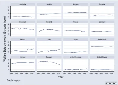
In order to measure the economic policy that deals with income protec-tion, we use a global index of generosity of the welfare state (Figure 1)

cal-culated by Scruggs (2004)8. This index is a computation of net replacement

rates of unemployment bene…ts, sickness bene…ts and pension insurance, the extent of program coverage and duration -it is actually an extension of the decommodi…cation index of Esping-Andersen (1990). The advantage of this index is that it gives a better idea of the willingness of the States to protect income than the ratio of social expenditures to GDP, since it encompasses not only generosity scores, but also measures of access conditions.

5_{A similar argument is developed by Lijphart (1994) when describing parliamentary}

systems as consensus democracies.

6_{Australia, Austria, Belgium, Canada, Denmark, Finland, France, Germany, Ireland,}

Italy, Japan, Netherlands, Norway, Portugal, Spain, Sweden, United Kingdom and USA.

7_{We use data from the following ISSP modules “Social Inequality I, II and III” and}

“Role of Government I, II and III” that took place in years 1985, 1987, 1990, 1992, 1996 and 1999 (data available at www.gesis.org).

8_{Scruggs’ Overall Generosity Score is available on his website. See also Allan and}

The political demand is here de…ned as being the share of people who agree with government redistribution (Figure 2). More precisely, it is the share of individuals, by year and by country, who agree or strongly agree while answering to the following ISSP survey question (Table 14):

“What is your opinion of the following statement: It is the re-sponsibility of the government to reduce the di¤erences in income between people with high incomes and those with low incomes” Possible answers rank from 1 (strongly agree) to 5 (strongly disagree). The higher the measure of the demand, the higher the number of people who

agree with redistribution9_.

The heterogeneity of the political demand is de…ned as being the coe¢ -cient of variation of preferences for redistribution (Figure 3): It is a measure of dispersion of the within-country distribution of answers, based on the dis-agregated data of micro surveys (Figures 4 to 9). We …rst calculate the standard deviation, for each survey year and each country, of answers to the question on redistribution; we then divide the standard deviation by the

country mean answer, in order to have a scale-free measure of dispersion10:

CV = pi;t

pi;t

with the standard deviation of the distribution of preferences pi;t and

the mean preferences, by country i and year t. We are thus able to compare

the dispersion of answers in countries with very di¤erent mean preferences11.

9_{In order to have a demand variable that is continuous, and given that mean preferences}

by country are slowly changing over time, we interpolate the missing points between two surveys and suppose that the demand is invariant over the beginning period 1980-1985. Several robustness check have been done (using the mean answer of individuals with and without weights, using the median answer, dropping some time span), which do not a¤ect the results.

10_{We could also take advantage of a measure of the asymmetry of the distribution of}

preferences by country, either proxied by the di¤erence between the mean and the median divided by the standard deviation of the distribution (Pearson’s skewness), or calculated with respect to the third moment about the mean (Fisher’s skewness). However, since the distribution of preferences is systematically skewed to the right in our sample (mean > median), results are similar to those obtained using the mean level of preferences.

11_{As a robustness check, we also computed the index of ordinal variation (I.O.V.) instead}

The higher the CV, the more heterogeneous within-country preferences for redistribution.

Finally, the fractionalization of the party system is taken from Armingeon et al. (2004) and measured according to the formula of Rae (1967):

F = 1 m X

i=1 t2_i

with ti the share of votes for party i and m the number of parties (Figure

10). The higher the Rae’s index, the more fractionalized the party system (the higher the number of parties).

As for controls, we include in our regressions the government’s ideological position in the left-right spectrum (continuous variable) weighted by votes, calculated by Amable, Gatti and Schumacher (2006) using information from Cusack and Engelhardt (2002) database. This database builds itself on the Comparative Manifesto Project (Budge et al., 2001). The standardized un-employment rate (OECD) is used as an additional macroeconomic control, along with a measure of productivity (GDP per employed worker based on US dollars 2002, OECD). Productivity enters the regression in natural logarithm and with a 1 period lag, in order to limit collinearity with the unemployment rate12.

Our time-series cross-section data set contains 18 OECD countries over 23 years. However, only 15 countries participated to the ISSP modules we are interested in to construct our demand variable. Indeed, Belgium and Finland did not participate, and data for Denmark are available only for the last wave (year 1999), on a non standardized separate data set. We did not include it in the analysis. Nor did we include Netherlands and Portugal, since the ISSP data were available only for the year 1999, implying a

time-invariant demand for redistribution over the entire period13_{. Finally, when}

fall into one category, and 1 when extreme polarization is present. In our sample, it varies from 0:47 to 0:79. The correlation between the index of ordinal variation and the standard deviation of our demand variable is 98%. This conforts our assumption of continuous preferences. Hence, considering that the standard deviation is a more popular concept, and since results are not a¤ected at all by the choice of the measure of dispersion, we only report regressions using the coe¢ cient of variation based on standard deviation.

12_{We also checked for the inclusion of a measure of in‡ation and budget de…cit, but}

these never turned out to be signi…cant, so we do not include them in the …nal regressions.

13_{As a robustness check, we included Netherlands in the sample. Results are left}

dealing with the generosity score of the welfare state constructed by Scruggs (2004), data for Portugal and Spain are not available. We eventually run the regressions for 12 countries over the time span 1980-2002 (Table 13).

4

Estimation Strategy and Basic Results

As a baseline model, we …rst estimate a naive pooled OLS model, which does not take into account the panel structure of our data. OLS assumes spherical errors (homoskedasticity and independence of the errors), a strong assumption which, if not hold, keeps OLS estimates unbiased but renders them ine¢ cient. Hence, we systematically compute panel corrected standard errors (PCSE) that takes into account panel-level heteroskedasticity and

contemporaneous spatial correlation, following Beck and Katz (1995)14_.

4.1

Model Speci…cation

Our baseline model is the following:

yit = + 1fit+ 2pit+ 12fitpit+ it (1)

where it is the i.i.d. error term

yit being the overall generosity score of the welfare state, which is

de-…ned by country i and by year t, fit being the level of party fractionalization

measured by the Rae formula, pit being either the level or the coe¢ cient of

variation of preferences for redistribution, and fitpitbeing the interaction

be-tween party fractionalization and preferences (level or dispersion). In other words, we test a reduced form of a relationship with a complementarity

ef-fect. Since we run an OLS estimate, is a single intercept that re‡ects the

expected value of the dependent variable when all of the independent vari-ables are zero.

14_{Importantly, the authors show the superiority of PCSE estimates over GLS estimates}

when T is not signi…cantly higher than N. Indeed, when T does not tend to in…nity, as is the case in our dataset, the Park method (GLS estimate) yields standard errors that are too small -up to 600 percent- and therefore overcon…dent results. By contrast, so long as T > 15 (which is our case, since T = 23), Monte Carlo experiments show that PCSEs are considerably better than OLS standard errors when there is panel heteroskedasticity and contemporaneous correlation of the errors.

In a second speci…cation of our model, we add some of the controls usually found in the literature:

yit = + 1fit+ 2pit+ 12fitpit+ 1uit+ 2wit 1+ 3git+ t+ it (2)

uitbeing the unemployment rate, wit 1being the log of labor productivity

lagged once (in order to limit collinearity with the unemployment rate) and git

being a measure of the partisanship of the government (continuous left-right

index)15_{. Moreover, while adding time dummies}

t, we control for additional

(macroeconomic) shocks that are common to all countries16.

4.2

Interaction Term and Marginal E¤ect

Since we consider an interaction term between fractionalization and

prefer-ences (fitpit) in equations (1) and (2), the assessment concerning the expected

overall e¤ect of pit needs the computation of its marginal e¤ect conditional

on speci…c values of fit:

@E(yit=x)

@pit

= b₂+ b₁₂fit (3)

given that x is the vector of explanatory variables.

Hence, it is worth to notice that a positive and signi…cant ₂ in equations

(1) and (2) means nothing but that preferences for redistribution increase the generosity of the State, only for those countries where the degree of party

fractionalization is zero (fit = 0) (Mullahy, 1999; Braumeoller, 2004). That

is for the unrealistic case of a single-party legislature17_{. Similarly, in order}

to assess the signi…cance of the e¤ect of pit on yit conditional on fit values,

15_{It is worth to notice that we do not include a measure of age dependency (e.g. share}

of the population below 15 or over 65), since this would be strongly correlated with our demand variable, which is precisely the reason why it is usually included in the literature given that scholars try to proxy the demand (Tabellini, 2000).

16_{We also checked for the existence of non linear relationships between variables, as it}

would make sense according to our descriptive statistics (Figures 11, 12 and 13). To do this, we applied a logarithmic transformation to our dependent and continuous independent variables in equation (1). Results are globally the same as those obtained with a linear approximation, so we do not report them here.

17_{This case, actually, could be achieved through a dictatorship, but since we only include}

the standard error of the sum ( 2+ 12fit)will be computed in the following way: se = q var(b₂) + f2 itvar(b12) + 2fitcov(b2b12) (4)

Keeping in mind that the coe¢ cient and standard errors that appear in the output of the regressions are partial ones -and not general ones like in an addi-tive model-, it is not surprising that statistically insigni…cant (and negaaddi-tive) coe¢ cients might combine to produce statistically signi…cant (and positive) overall e¤ects (Friedrich, 1982). Hence in the following, we systematically report marginal e¤ects of preferences for redistribution at di¤erent sample values of party fractionalization (minimum, mean minus one standard devia-tion, mean, mean plus one standard deviadevia-tion, maximum). We also compute the marginal e¤ects of party fractionalization at di¤erent sample values of preferences.

4.3

Basic Results

Tables 1 to 3 show the result of the baseline regressions, using the level of the demand for redistribution as our independent variable of interest. In this naive OLS estimates, we add variables step by step (Table 1): …rst, we test a linear model without the complementarity e¤ect (column [1]), then we add the interaction term (column [2]), macroeconomic and political controls (column [3]) and …nally time dummies (column [4]).

We are especially interested in the marginal e¤ect of the demand for redistribution on the welfare state generosity (Table 2). When signi…cant, this marginal e¤ect is always positive (column [1] Table 1, columns [2], [3] and [4] Table 2) and increases with the level of party fractionalization when controls are included (columns [3] and [4] Table 2). As for the overall impact of party fractionalization, we also notice a positive impact on welfare state generosity (column [1] Table 1, columns [2], [3] and [4] Table 3): The more fractionalized the party system, the higher the welfare state generosity. This e¤ect is enhanced by the level of the demand, as soon as standard controls are included in the regression (columns [3] and [4] Table 3).

We conclude from this …rst set of basic results that there is a positive relationship between the level of the demand for redistribution and the gen-erosity of governments, and between the degree of party fractionalization and the generosity of governments. Importantly, demand for redistribution and party fractionalization are complementary: An increase in the former

enhances the positive impact of the latter on welfare state generosity, and vice versa.

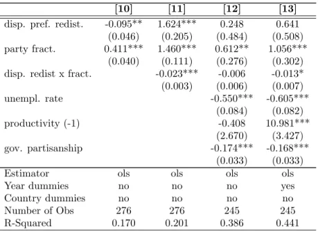
Turning to our second set of regressions, we aim to measure the impact of the dispersion of preferences for redistribution on the welfare state generosity (Tables 7 to 9). It comes out that -contrary to our expectations- the het-erogeneity of the demand has a negative impact on welfare state generosity (Table 8). Moreover, the higher the fractionalization of the party system, the larger the negative impact of preferences dispersion. However, looking at party fractionalization, the variable appears to maintain its strong positive impact on welfare state generosity (Table 9). It is worth to notice here that the above results are produced by pooled OLS, which do not take into ac-count the particular structure of our cross-section time-series dataset, hence lead to potentially biased estimates.

5

Criticisms and Further Results

There are a number of problems coming with the use of cross-section time-series data. Below, we discuss some of them and the solutions we adopted to deal with them. Speci…cally, we explain our choice of including …xed e¤ects into the model, hence consciously restricting our insight to intra-country variation (Section 5.1). Then, we deal with the issue of correctly estimating the impact of time-invariant variables while keeping …xed e¤ects into the model (Section 5.2). We further deal with dynamic issues and measure the speed of adjustment of the welfare state (Section 5.3).

5.1

Introducing Fixed E¤ects

Country …xed e¤ects control for characteristics that are speci…c to one coun-try and do not vary across time. Such a speci…cation takes advantage of the time-series cross-section nature of our dataset.

5.1.1 Model Speci…cation with Fixed E¤ects

The inclusion of …xed e¤ects allows for unobserved heterogeneity. Instead of

a single intercept , each cross-sectional unit is assigned its own intercept _i.

Since our estimated …xed e¤ects are always large and clearly signi…cant, not including them in the model would result in a presumably serious omitted

variable bias (Green, Kim and Yoon, 2001). However, it is worth to notice that while including …xed e¤ects we limit our interest to the causes of intra-country variation of welfare state generosity.

Hence, equations (1) and (2) become:

yit = 1fit+ 2pit+ 12fitpit+ t+ i+ it (5)

yit= 1fit+ 2pit+ 12fitpit+ 1uit+ 2wit 1+ 3git+ t+ i+ it (6)

where _i represents the country unit e¤ect and _it is the i.i.d. error term.

5.1.2 Heteroskedasticity and Spatial Correlation

There are a number of statistical properties to verify while using the …xed e¤ects model.

First, cross-section correlation (spatial correlation) is a problem for …xed e¤ect estimation. Then, after running a standard …xed e¤ect model, we look at the Breusch-Pagan statistic that tests for cross-section independence in

the residuals18_{. Indeed, a …xed e¤ect model assumes the independence of the}

errors. A likely deviation from independent errors in the context of pooled cross-section time-series data is the presence of contemporaneous correlations across cross-sectional units (here across countries). The null hypothesis of

the Breusch-Pagan test is that of cross-sectional independence19_{. The test}

rejects the null hypothesis20, hence there is spatial correlation in our data.

Second, a …xed e¤ect model assumes homoskedasticity. The most likely deviation from homoskedastic errors in the context of pooled cross-section time-series data like ours is the presence of error variances speci…c to the cross-sectional unit. Therefore, we calculate a modi…ed Wald statistic for

18_{We use the xttest2 Stata command, following Greene (2000).}

19_{In the context of a slightly unbalanced panel like ours, the observations used to}

cal-culate the test statistic are those available for all cross-sectional units. Here, the number of available observations reported is 16.

20_{Breusch-Pagan LM test of independence:} 2_{(66) = 158:526, p < 0:01 for the model}

with the level of demand, and 2_{(66) = 145:016, p < 0:01 for the model with the dispersion}

groupwise heteroskedasticity in the residuals of a …xed e¤ect regression model21_.

The null hypothesis of homoskedasticity is strongly rejected22.

Thus, the above tests suggest that we might not use the standard …xed e¤ect procedure without taking into account spatial correlation and panel heteroskedasticity. As a consequence, we run least squares dummy variables (LSDV) regressions (i.e. the unobserved e¤ect is brought explicitly into the model) that allow us to compute panel corrected standard errors (PCSE).

5.1.3 Results of Fixed E¤ects Regressions

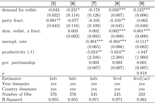
Results concerning the impact of the demand for redistribution in level on the welfare state generosity are shown in Tables 4 to 6, columns [5], [6] and [7]. As a start, we notice that the R-squared are highly raised by the inclusion of …xed e¤ects: Our …xed e¤ects model is able to explain more than 95% of

the sample variation. Moreover, …xed e¤ects are strongly signi…cant23, which

means that not including them into the regression leads to an important omitted variable bias (Green, Kim and Yoon, 2001).

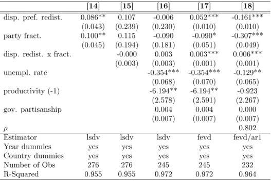
Although it is not possible to theoretically assess the direction of the bias, we clearly see the empirical di¤erence between the coe¢ cients of Table 1 and those of Table 4 (the comparison is especially meaningful between columns [4] Table 1 and [7] Table 4 that include the full set of controls). The same comments apply to our regressions measuring the impact of the dispersion of preferences on the welfare state generosity (Tables 10 to 12, columns [14] to [16]).

Looking at control variables …rst, the impact of unemployment on welfare state generosity remains negative and highly signi…cant, but is half-size. The coe¢ cient of productivity becomes negative and signi…cant, and increases in size. Surprisingly, the coe¢ cient of government partisanship turns positive and is no more signi…cant: This means that the position of the government on the political (left-right) spectrum has no impact on the within-country variation of welfare state generosity. Taking the result seriously, it means that once we control for the preferences (of voters) for redistribution and the degree of party fractionalization (hence, the occurence of coalitions),

21_{We use the xttest3 Stata command, following Greene (2000).}

22_{Modi…ed Wald test for groupwise heteroskedasticity:} 2_{(12) = 457:44, p < 0:01 for}

the model with the level of demand, and 2_{(12) = 1092:01, p < 0:01 for the model with}

dispersion of preferences.

government partisanship does not play any role in the size of government. This runs counter to other studies on partisanship that show a strong impact of the ideological position of governements on public expenditures (Huber, Ragin and Stephens, 1993).

Looking at our key variables, two important results show up:

(i) The impact of the demand for redistribution, which is a slowly changing

variable, is entirely captured by country …xed e¤ects: The coe¢ cients of columns [6] and [7] Table 5 cannot be distinguished from 0 -although we still capture the complementarity e¤ect between the demand and

party fractionalization24_.

(ii) The impact of the dispersion of preferences for redistribution, which

is also a slowly changing variable, resists the introduction of country …xed e¤ects: The coe¢ cients of columns [15] and [16] Table 11 are

positive and signi…cant25_{. Moreover, once controls are included in the}

regression, we capture the complementarity e¤ect between dispersion of preferences and party fractionalization.

(iii) The e¤ect of party fractionalization on welfare state generosity is strongly

decreased by the inclusion of …xed e¤ects (columns [6] and [7] Table 6 and columns [15] and [16] Table 12): Except when the demand for redistribution (in level or in dispersion) is at its maximum value, we merely …nd an impact of party fractionalization (the e¤ect vanishes when controls are included).

5.2

Coping with Time-invariant Variables and Fixed

E¤ects

Our measure of preferences (pit), be it in level or in dispersion, is considered

as a rarely changing variable. This means that the demand for redistribution

24_{Interestingly though, the impact of the demand for redistribution on welfare state}

generosity is negative and signi…cant when party fractionalization is at very low levels. However, we have no explanation for this, except that running a …xed e¤ects regression with slowly changing variable leads to ine¢ cient estimates (Beck and Katz, 1995; Plümper and Troeger, 2007).

25_{Importantly, here we measure the within-country impact of dispersion, whereas}

previ-ous OLS regressions measured the pooled impact of dispersion on welfare state generosity. However, the omitted variable bias appears to be strong in OLS regressions.

is almost time-invariant or at least cross-sectionally dominated (Figure 2). Indeed, as shown in the Appendix (Table 13), the between variance is more than 3 times higher than the within variance. Hence, we are confronted to the well-known problem of estimating a …xed e¤ects model with (almost) time-invariant variables. The problem comes from the fact that all the e¤ect of the

time-invariant variables is likely to be captured by the unit …xed e¤ects26_.

To deal with this issue, we make use of the estimator proposed by Plümper and Troeger (2007): A three-stage panel …xed e¤ects vector decomposition model (FEVD procedure).

5.2.1 Fixed E¤ects Vector Decomposition Procedure

The FEVD process allows for the inclusion of time-invariant variables and ef-…ciently estimates almost time-invariant explanatory variables within a panel …xed e¤ects framework (Plümper and Troeger, 2007). More precisely:

(i) The …rst stage estimates a pure …xed e¤ects model in order to obtain an

estimate of the unit e¤ects (here our country e¤ects _i).

(ii) The second stage decomposes the …xed e¤ects vector into a part

ex-plained by the time-invariant or almost time-invariant variables (here

our demand for redistribution pit) and an unexplainable part -the error

term of the second stage.

(iii) Finally, the third stage re-estimates the original model by pooled OLS,

including the error term of the second stage. This third step assures to control for collinearity between time-varying and invariant right-hand side variables, and adjusts the degrees of freedom.

To complement the estimation process, we apply panel corrected standard errors (PCSE) to the third stage pooled OLS.

26_{Actually, the problem of almost time-invariant variables with …xed e¤ects is slightly}

di¤erent from the issue raised by time-invariant variables with …xed e¤ects. As explained by Plümper and Troeger (p.16, 2007), “When the within variance is small, the FE model does not only compute large standard errors, but in addition the sampling variance gets large and therefore the reliability of point predictions is low and the probability that the estimated coe¢ cient deviates largely from the true coe¢ cient increases.”

5.2.2 Results of FEVD Estimates

Results for the level of the demand are shown in Tables 4 to 6, column [8]. We notice that the main impact of applying the FEVD procedure is to change the coe¢ cient of the almost time-invariant variable, while letting the other

coe¢ cients unchanged27_{. The marginal e¤ects of the demand for}

redistrib-ution calculated in Table 5 for di¤erent values of party fractionalization are positive and highly signi…cant. They increase with the fractionalization of the party system. Hence, the demand for redistribution is shown to have a strong impact on welfare state generosity.

Results for the dispersion of preferences are shown in Tables 10 to 12, column [17]. The marginal e¤ects of the dispersion of preferences for redis-tribution calculated in Table 11 for di¤erent values of party fractionalization are positive and highly signi…cant. They increase with the fractionalization of the party system. We notice that the results obtained by FEVD estimates (column [17]) are very close to the one obtained by FE estimates (column [16]).

However, due to the fact that almost time-invariant variables are esti-mated by quasi-pooled OLS in the second stage, their coe¢ cients are possi-bly biased, depending on their correlation with the unobserved unit e¤ects (Plümper and Troeger, 2004). The bias is positive (negative) if the rarely changing variables covary positively (negatively) with the unit …xed e¤ects. The importance of the bias depends on the size of the correlation and on the size of the between-to-within ratio of the rarely changing variable: The smaller the actual correlation and the larger this ratio, the smaller the actual bias. Plümper and Troeger (2007) run Monte-Carlo estimates to identify the conditions under which the FEVD procedure is preferable to the FE esti-mates. They show that if there is no correlation between the rarely changing variable and the unit country e¤ect, the between-to-within ratio can be as small as 0:2; it the correlation is 0:3, the ratio should be larger than 1:7; at a correlation of 0:5, the threshold increases to about 2:8.

Running the correlation matrix between our variables of interest and the estimated unit e¤ects (after the …xed e¤ects model of the …rst stage), we …nd correlations of 0:32 (demand for redistribution) and 0:04 (dispersion of preferences). We know from Table 13 that the between-to-within ratio of our

27_{Indeed, the coe¢ cients of the time-varying variables are still estimated by a standard}

slowly changing variables is 3:46 if we consider the demand for redistribution (i.e. two times the recommanded threshold of 1:7), and as big as 2:90 if we consider the dispersion of preferences for redistribution. Hence, our FEVD estimates are undoubtedly consistent and we can be con…dent in our results.

5.3

Dynamic Issues

Following our descriptive statistics, we suspect some path dependency re-garding the overall level of generosity of the welfare state (Figure 1). More-over, the panel corrected standard errors that we calculate in our regressions assume that the disturbances are heteroskedastic and contemporaneously correlated across panels, but that there is no serial autocorrelation. There-fore, for our estimates to be precise, we must take care of a potential serial autocorrelation.

5.3.1 Dynamic Model Speci…cation

We test for serial autocorrelation using the Wooldridge test for

autocorre-lation in panel data28. The test strongly rejects the null hypothesis of no

…rst-order autocorrelation29_{. Hence, we have two options: (i) Treating the}

model as static and purging any temporal correlation or (ii) Explicitely using the dynamics.

(i) If we treat the model as static and the temporal correlation as a problem,

we assume that the latter has no substantive interest. Then, the point

is to estimate and to use it to correct the errors. This is the AR(1)

error model:

yit = 1fit+ 2pit+ 12fitpit+ t+ i+ it (7)

where it = it 1+ it,

or equivalently _it= yit 1 k xkit 1+ it

(ii) If we are interested in a dynamic speci…cation of the model, we can

explicitly include the lagged dependent variable (LDV) into the model:

yit = yit 1+ 1fit+ 2pit+ 12fitpit+ t+ i+ it (8)

28_{We use the xtserial Stata command, following Wooldridge (2002) and Drukker (2003).}

29_{Wooldridge test for autocorrelation in panel data: F (1; 11) = 28:257, p < 0:01 for}

the model with the level of demand, and F (1; 11) = 25:025, p < 0:01 for the model with dispersion of preferences.

With such a speci…cation, we should get rid of the error autocorrelation, since the lagged dependent variable includes lagged error term (Beck and Katz, 2004). Contrary to the AR(1) speci…cation that allows a quick adjustment of the dependent variable, here we explicitely measure long-term e¤ects or slow adjustment of the dependent variable to a change in the independent variables.

We have no a priori expectations on the speed of adjustment of our dependent variable. However, the …xed e¤ect vector decomposition estimator

can only take into account the AR(1) error process30. Not knowing the

resulting bias in the LDV speci…cation, we therefore choose to run an AR(1) model.

5.3.2 Dynamics with Fixed E¤ects: the Nickell Bias

The inclusion of a lagged dependent variable with …xed e¤ects, be it implicit

or explicit, raises new issues. Indeed, it induces a correlation between ^y,

the lagged dependent variable in terms of deviation from its mean (^yit 1 =

yit 1 _T1

P

yit 1) and ^, the error term in terms of deviation from its mean

(^it 1 = it 1 T1

P

it 1). Hence it leads to biased estimates (Nickell,

1981): There is a downward bias while estimating , and an upward bias in

the estimations of .

To deal with this issue, many alternative estimators have been proposed in the econometric literature. However, all of them are speci…cally designed for panel data (T < 10 and N very large), not for TSCS data (T > 20 and N < 30)31.

Beck and Katz (2004) produce Monte Carlo experiments for TSCS alike data. Adding a correlation between the unit e¤ects and the exogenous vari-ables, they aim to compare the performance of the LSDV estimator includ-ing a lagged dependent variable, with the Anderson-Hsiao estimator and the

30_{Indeed, no correction is applied to the error of the second stage while running an LDV}

model, though this second-stage error is to be used in the third stage OLS estimate. By opposition, the FEVD procedure has been designed to apply the AR(1) Prais-Winsten transformation in the …rst and third stages.

31_{For instance, the instrumental variables procedure suggested by Anderson and Hsiao}

(1982) might be at the cost of raising dramatically the mean squared error (Beck and Katz, 2004); GMM (Arellano and Bond, 1991) only works if N is very large; Kiviet (1995) approach assumes the data are balanced, among other important issues that do not …t our data.

Kiviet correction, as both T and vary (the other parameters are …xed at a single value, with N = 20). Results are the following. The authors show clear evidence that there is a downward bias using the LSDV estimator, which dramatically decreases with T and slightly increases with . Moreover, the authors give strong advice not to use the Anderson-Hsiao estimator for TSCS data, the cost of using it being very high in terms of root-mean square error (namely, the estimation variability is very high). Finally, they advise to use the LSDV estimator preferably to the Kiviet correction as long as T > 20, which is our case (Table 13).

Consequently, when testing the dynamic speci…cation of the model, we stay with our FEVD estimator, which has the advantage of being able to estimate the coe¢ cient of the slowly-changing variable of interest, namely the political demand. We apply the AR(1) error model de…ned in equation (7) and assess the speed of adjustment of the generosity of the welfare state.

5.3.3 Unit Roots

Before to turn to the results, a last check should be done concerning the presence of unit roots in the data (non-stationarity). Indeed, if our dependent variable is not stationary, the introduction of a lagged dependent variable to model dynamics will lead to spurious regressions. We thus run a battery of unit roots tests.

Following Maddala and Wu (1999), we run a Fisher test, which assumes that all series are non-stationary under the null hypothesis against the alter-native that at least one series in the panel is stationary. Alteralter-native tests are those proposed by Levin, Lin and Chu (2002) (hereafter LL) and Im, Pesaran and Shin (2003) (hereafter IPS). Under the null hypothesis that all series are non-stationary, the test proposed by Levin, Lin and Chu (2002) supposes that the autoregressive coe¢ cient ( ) is the same for all units. Hence, the LL test is based on pooled regression and only …ts balanced panel. Under the same null hypothesis, the test proposed by Im, Pesaran and Shin (2003) improves the LL test by relaxing the assumption of a common : the IPS test runs a separate unit test for each of the units and computes the mean of the t-statistic of each independent Augmented Dickey-Fuller test. IPS …ts only balanced data with the same number of observations per unit. Finally, we can see the Fisher test developed by Maddala and Wu (1999) as an im-provement of the IPS test: it also runs individual tests but then combines their signi…cance with a Fisher test. Hence, it does not require a balanced

data. The Fisher test of Maddala and Wu (1999) and the IPS test of Im, Pesaran and Shin (2003) are directly comparable. Since our data is only

slightly unbalanced, we compute both statistics32_{. Results are in Table 15.}

Moreover, after estimating the dynamic version of the model, we system-atically check whether the residuals appear stationary. To do that, we run an autoregression of the residuals on their lags and check if the coe¢ cient of the lagged residuals is close to one. Finally, we also run a series of autoregression for all our variables, thus examining the size of the coe¢ cient of the lagged variables (Beck, 2006). We conclude that there is no unit root in our panel.

5.3.4 Results of Dynamic Regressions

Tables 4 to 6 column [9] give the results of the estimates. We notice the

non trivial value of ( = 0:82), which con…rms the existence of a

conver-gence mechanism of the welfare state of each country towards its long term

value ( i

1 ) (Bond, 2002; Beck and Katz, 2004). In other words, the initial

deviation of the welfare state from its stationary value is very low (Blundell and Bond, 1998). Indeed, the past level of the welfare state helps to explain the current level: Radical reforms of the welfare state -like going, within a country, from the level of the US to the level of Sweden- are not common.

However, the short term e¤ect of the demand is still sizeable. Moreover, we continue to capture the complementarity between the political demand and the fractionalization of parties (Table 5): The higher the fractionalization of the party system, the better the demand for redistribution is conveyed to the policy implemented by the government. Importantly, the marginal e¤ects of the demand are very comparable to the ones obtained in the static speci…cations of the model discussed above. Hence, this reinforces our results.

6

What Have We Learned?

Since we are interested in the joint e¤ect of (the fragmentation of) the de-mand with the fractionalization of the party system, we systematically in-troduced an interaction term into our regressions. Conducting the analysis, we seek to know to what extent the level of generosity of the welfare state

32_{We use the xt…sher Stata command to compute the Fisher test, and the ipshin Stata}

depends on the level (or the dispersion) of the expressed demand for redistri-bution and on the degree of atomicity of the political supply. We argue that the impact of the demand should be positive and increase with the number of parties.

6.1

What Drives the Generosity of the Welfare State?

In Tables 1 to 6 that test the argument according to which the level of the demand for redistribution determines the generosity of the welfare state, we …nd indeed that the marginal e¤ect of the demand, always very signi…cant, is positive and increases with the degree of fractionalization of political parties (Table 5). If taken in isolation, the impact of the fractionalization of the supply on the generosity of the State is positive, but becomes signi…cant only when the demand for redistribution is above the mean (Table 6). These results have two important implications:

(i) The political demand is indeed conveyed to the political arena, since it

has a direct impact on the level of generosity of the State, even when the fractionalization of the political supply is weak (in other words, democracy works well). In addition, the political demand and the frac-tionalization of parties are complementary.

(ii) The fractionalization of political parties has a positive impact on the

welfare state only to the extent that it exists a relatively high de-mand for redistribution. Hence, contrary to what has been found in the literature (Milesi-Ferretti, Perotti and Rostagno, 2002; Bawn and Rosenbluth, 2006), we do not …nd strong evidence of a direct impact

of the fractionalization of parties on the size of government33.

33_{Milesi-Ferretti, Perotti and Rostagno (2002) use data for 20 OECD countries over the}

period 1960-1995. They look at the impact of a macro shock at di¤erent level of pro-portionality of the political system on the spending/GDP ratio and on the transfer/GDP ratio (OECD data). They conclude that the higher the proportionality of the system, the higher the impact of a macro shock on the public spending. Bawn and Rosenbluth (2006) use data for 17 Western European countries over the period 1970-1998. They look at the impact of the number of parties in government (extracted from the database of Warwick, 1994) on the overall government expenditure as a fraction of GDP in a given year (OECD data). They …nd a positive impact of the number of parties in government on the overall government expenditure.

6.2

How is the Heterogeneity of Preferences Conveyed

by Party Fractionalization?

We now turn to our second set of regressions, which assess the impact of the dispersion of preferences. Here, we test the idea that the fragmentation of the political demand, measured by its coe¢ cient of variation, has a positive impact on the generosity of the welfare state. This impact is assumed to increase with the fractionalization of the party system. Tables 7 to 12 give the results of regressions. The marginal e¤ect of the dispersion of preferences is indeed positive, increasing with Rae’s index (party fractionalization), and highly signi…cant (Table 11): The generosity of the government is higher when the demand is spread out, and the fractionalization of parties helps to

convey the dispersion of this demand34_{. We add two important comments}

on the results:

(i) Results are robust to the choice of the estimation process (…xed e¤ect

vec-tor decomposition or OLS with country dummies and panel corrected standard errors). Even if the unit …xed e¤ect partly captures the im-pact of the demand when running an OLS with country dummies, the coe¢ cient of preferences dispersion remains positive and signi…cant.

(ii) The impact of the dispersion of preferences on the generosity of the

wel-fare state increases very rapidly with the degree of the fractionalization of parties: It more than doubles in the dynamic speci…cation, when the fractionalization varies from its minimum value to its maximum value. Hence, the parallelism between heterogeneity of preferences and abun-dance of the political supply seems relevant.

Some comments on the control variables. First, we notice that the co-e¢ cient of the ideological position of governments never turns out to be signi…cant, once country …xed e¤ects are included. This would suggest that governments directly encompass the demand within their policy decision, and have themselves no preferred policy. But we could also assume that the parti-san position of governments, due to a feedback e¤ect, is already captured by the term which expresses individual preferences (Gerber and Jackson, 1993).

34_{We notice in addition that the size of the overall e¤ect of party fractionalization is}

Concerning the macroeconomic controls, we notice that the unemployment rate acts negatively on the index of generosity of the welfare state. We inter-pret this as a downward adjustment of the replacement rates to an increase in the number of bene…ciaries (see Amable, Gatti and Schumacher, 2006 for evidence on this point).

6.3

How Large is the E¤ect?

In order to interpret these results, it is important to get some sense of the magnitude of the e¤ect.

How Large is the Impact of the Demand? Other things being equal,

raising by 10% the number of people who agree with redistribution implies: An increase of 3:2% of the welfare state generosity score, when the number of political parties (Rae’s index) is at its minimum (2 parties); An increase of 5:3% when the number of political parties reaches its maximum value (10 parties). Taking dynamics into account, these …gures become 4% and 5%, respectively. Hence, the political demand has a non trivial impact on public policy outcome.

How Large is the E¤ect of the Dispersion of Preferences? Other

things being equal, raising by 10% the coe¢ cient of variation of preferences for redistribution implies: An increase of 3:7% of the welfare state generosity score, when the number of political parties (Rae’s index) is at its minimum (2 parties); An increase of 5:4% when the number of political parties reaches its maximum value (10 parties). Taking dynamics into account, these …gures become 2:9% and 6:7%, respectively. We conclude that within-country het-erogeneity of the demand is highly conveyed by party fractionalization.

Finally, an increased competition between parties bene…ts the electorate: The demand of the electorate is better re‡ected in the policy formation when parties are numerous.

7

Conclusion

This paper proposes an empirical analysis of the interaction between the demand for redistribution expressed by individuals and the structure of the

political supply. Hence, con‡ictual demands of heterogeneous agents can …nd a way to be expressed in public policies, according to the design of the political mediation. The latter partly depends on political institutions, namely election rules and the structure of the political supply. This implies that the matching of the supply to the political demand determines the nature of the welfare state, speci…cally the level of redistribution. We thus expect the structure of the party system to impact the generosity of the State, while allowing or not heterogeneous demands for redistribution to be taken into account. In particular, a more fractionalized party system will raise the representativity of elected bodies and enhance the re‡ection of political demand that comes from lower and middle class. Consequently, the higher the fractionalization of the party system, the better re‡ected the demand for redistribution into social policy outcomes. As far as we know, the empirical literature on the subject only tests the in‡uence of the supply on the nature of public expenditures (Persson and Tabellini, 1999). No test of an interaction between a feature of the political supply and the political demand has been done.

The originality of the present work is then (i) to use a direct measure of individual voter preferences, (ii) to analyze the composition e¤ect of the demand on policy outcome, and (iii) to take into account the interaction between the demand for redistribution and the structure of the political sup-ply. This is done to explain the level of generosity of the welfare state and its variation within countries. Econometric regressions use time-series cross-section data on a sample of 18 OECD countries spanned over the period 1980-2002. The data originates from both microeconomic databases (pref-erences for redistribution) and macroeconomic databases (policy outcome, party fractionalization).

Results clearly show that the demand for redistribution, measured in level and in dispersion, leads to a more generous welfare state, the more the party system is fractionalized (the higher the number of parties in Parliament). This is robust to a large variety of econometric speci…cations.

Yet, as Shepsle and Weingast (p.50, 1984) put it: “Each of the above conclusions depends upon a rather special sort of preference revelation. Indi-vidual agents are assumed to be sincere revealers of their preferences so that the majority preference relation (built up from sincerely revealed individual preferences) may be taken as descriptive of the voting behaviour of majori-ties”. This is a strong, though necessary, assumption that we have done in

this study.

Importantly, concerning the aggregation of preferences, we made a sim-plifying assumption by giving the same weight to each individual preference (each person has one vote). This was necessary to generate conclusions at the macro level. However, assuming an alternative microfoundations for our model, we could extend our work. For instance, we could take into account the partisan positions at the individual level. Indeed, less ideological voters attract more attention from the parties, since they are considered as “swing voters” (Lindbeck and Weibull, 1987). We could then …nd a way to count

the number of swing voters in a group35_{. An extension would thus be (i)}

to gather preferences according to the social status or the occupation of in-dividuals, thus trying to form socio-political groups and (ii) to deduce the political weight of each group ex post, according to the dispersion of within-group preferences.

Finally, as in most empirical works with time-series cross-section data investigating the within country variation of variables, it would certainly be interesting to open the black box of country …xed e¤ect. A way to do it would be to enter more information on the institutional features of countries within the regression.

35_{Another way of infering di¤erent weights to people would be to identify lobbying}