HAL Id: hal-02636232
https://hal.inrae.fr/hal-02636232
Submitted on 27 May 2020
HAL is a multi-disciplinary open access
archive for the deposit and dissemination of sci-entific research documents, whether they are pub-lished or not. The documents may come from teaching and research institutions in France or abroad, or from public or private research centers.
L’archive ouverte pluridisciplinaire HAL, est destinée au dépôt et à la diffusion de documents scientifiques de niveau recherche, publiés ou non, émanant des établissements d’enseignement et de recherche français ou étrangers, des laboratoires publics ou privés.
Nonexclusive competition under adverse selection
Andrea Attar, Thomas Mariotti, François Salanie
To cite this version:
Andrea Attar, Thomas Mariotti, François Salanie. Nonexclusive competition under adverse selection. Theoretical Economics, Econometric Society, 2014, 9 (1), pp.1-40. �10.3982/TE1126�. �hal-02636232�
Nonexclusive Competition
under Adverse Selection
∗
Andrea Attar
†Thomas Mariotti
‡Fran¸cois Salani´e
§First draft: April 2010
This draft: October 2012
Abstract
A seller of a divisible good faces several identical buyers. The quality of the good may be low or high, and is the seller’s private information. The seller has strictly convex preferences that satisfy a single-crossing property. Buyers compete by posting menus of nonexclusive contracts, so that the seller can simultaneously and privately trade with several buyers. We provide a necessary and sufficient condition for the existence of a pure-strategy equilibrium. Aggregate equilibrium trades are unique. Any traded contract must yield zero profit. If a quality is actually traded, then it is efficiently traded. Depending on parameters, both qualities may be traded, or only one of them, or the market may break down to a no-trade equilibrium.
Keywords: Adverse Selection, Competing Mechanisms, Nonexclusivity. JEL Classification: D43, D82, D86.
∗We thank a coeditor, Johannes H¨orner, and two anonymous referees for very thoughtful and detailed
comments. We also thank David Bardey, Bruno Biais, Antoine Bommier, Catherine Casamatta, Pradeep Dubey, John Geanakoplos, Piero Gottardi, Martin Hellwig, David Martimort, Enrico Minelli, Alessandro Pavan, Nicola Pavoni, David P´erez-Castrillo, Gwena¨el Piaser, Jean-Charles Rochet, Bernard Salani´e, Larry Samuelson, Dimitri Vayanos, David Webb, and Robert Wilson for very valuable feedback. Finally, we thank seminar audiences at Collegio Carlo Alberto, Columbia University, ETH Z¨urich, European University Institute, Helsinki Center of Economic Research, London School of Economics and Political Science, Ludwig-Maximilians-Universit¨at M¨unchen, New York University, Princeton University, Rijksuniversiteit Groningen, Toulouse School of Economics, Universitat Pompeu Fabra, Universit´e de Cergy-Pontoise, Universit´e de Franche-Comt´e, and Universiteit van Tilburg, as well as conference participants at the 2011 CESifo Area Conference on Applied Microeconomics, the 2011 Conference of the Society for the Advancement of Economic Theory, the 2011 European Summer Symposium in Economic Theory, the 2011 IDEI/CSIO Workshop on Industrial Organization, the 2011 Toulouse Workshop of the Paul Woolley Research Initiative on Capital Market Dysfunctionalities, and the 2011 Universit¨at Z¨urich-ETH Z¨urich Workshop in Honor of Ivar Ekeland for many useful discussions. Financial support from the Agence Nationale de la Recherche (ANR–09–BLAN– 0358–01), the Chaire March´es des Risques et Cr´eation de Valeur, the European Research Council (Starting Grant 203929–ACAP), and the Europlace Institute of Finance is gratefully acknowledged.
†Toulouse School of Economics (IDEI, PWRI) and Universit`a degli Studi di Roma “Tor Vergata.” ‡Toulouse School of Economics (CNRS, GREMAQ, IDEI).
1
Introduction
The recent financial crisis has spectacularly recalled that the liquidity of financial markets cannot be taken for granted, even for markets that usually attract many traders and on which exchanged volumes tend to be very high. For instance, Adrian and Shin (2010) document that the issuance of asset-backed securities declined from over three hundred billion dollars in 2007 to only a few billion in 2009. Similarly, Brunnermeier (2009) emphasizes the severe liquidity dry-up of the interbank market over the 2007–2009 period, when many banks chose to keep their liquidity idle instead of lending it even at short maturities. It is tempting to associate these difficulties with asymmetries in the allocation of information among traders. Indeed, during the crisis, one of the banks’ main concern was the unknown exposure to risk of their counterparties.1 Moreover, structured financial products such as
mortgage-backed securities, collateralized debt obligations, and credit default swaps often involve many different underlying assets, and their designers are likely to hold private information about their quality; this creates an adverse selection problem that reduces liquidity provision.2
Finally, most of these securities are traded outside of organized exchanges on over-the-counter markets, with poor information on the trading volumes or on the net positions of traders. Hence agents are able to interact secretly with multiple partners, at the expense of information release. These two features, adverse selection and nonexclusivity, are at the heart of the present paper.
Theoretical studies of adverse selection in competitive environments have mainly been developed in the context of two alternative paradigms. Akerlof (1970) studies an economy where privately informed sellers and uninformed buyers act as price takers. All trades are assumed to take place at the same price. Competitive equilibria typically exist, but feature a form of market failure: because the market-clearing price must be equal to the average quality of the goods offered by the sellers, the highest qualities are generally not traded in equilibrium. It seems therefore natural to investigate whether such a drastic outcome can be avoided by allowing buyers to screen goods of different qualities. In this spirit, Rothschild and Stiglitz (1976) consider a strategic model in which buyers offer to trade different quantities at different unit prices, thereby allowing sellers to credibly communicate their private information. They show that low-quality sellers trade efficiently, while high-quality sellers end up trading a suboptimal, but nonzero quantity. For instance, on insurance
1See, among others, Taylor and Williams (2009), and Philippon and Skreta (2012).
2See Gorton (2009). There is also some evidence that lending standards and the intensity of screening have been progressively deteriorating with the expansion of the securitization industry in the pre–2007 years. See, for instance, Keys, Mukherjee, Seru, and Vig (2010), and Demyanyk and Van Hemert (2011).
markets, high-risk agents are fully insured, while low-risk agents only obtain partial coverage; no pure-strategy equilibrium exists if the proportion of low-risk agents is too high.
The present paper revisits these classical approaches by relaxing the assumption of exclusive competition, which states that each seller is allowed to trade with at most one buyer. This assumption plays a central role in Rothschild and Stiglitz’s (1976) model, and is also satisfied in the simplest versions of Akerlof’s (1970) model, in which sellers can only trade one or zero unit of an indivisible good. However, situations where sellers can simultaneously and secretly trade with several buyers naturally arise on many markets—one may even say that nonexclusivity is the rule rather than the exception. In addition to the contexts we have already mentioned, well-known examples include the European banking industry, the US credit card market, and the life insurance and annuity markets of several OECD countries.3
Our aim is to study the impact of adverse selection in markets with such nonexclusive trading relationships. To do so, we allow for nonexclusive trading in a generalized version of Rothschild and Stiglitz’s (1976) model. This exercise is interesting per se: as we shall see, the reasonings that lead to the characterization of equilibria are quite different from those put forward by these authors. The results are also different: the equilibria we construct typically feature linear pricing, possibly with a bid-ask spread, and trading is efficient whenever it takes place. On the other hand, pure-strategy equilibria may fail to exist, as in Rothschild and Stiglitz (1976), and some types may be excluded from trade, as in Akerlof (1970). It might even be that the only equilibrium involves no trade.
Our analysis builds on the following simple model of trade. There is a finite number of buyers, who compete for a divisible good offered by a seller.4 The seller is privately
informed of the quality of the good, which may be low or high. The seller’s preferences are strictly convex, but otherwise arbitrary, provided they satisfy a single-crossing property. Buyers compete by simultaneously posting menus of contracts, where a contract specifies both a quantity and a transfer. After observing the menus offered, and taking into account her private information, or type, the seller chooses which contracts to trade. Our model
3Detragiache, Garella, and Guiso (2000) and Ongena and Smith (2000) document that multiple banking relationships have become very widespread in Europe. Rysman (2007) provides recent evidence of multi-homing in the US credit card industry. Cawley and Philipson (1999) and Finkelstein and Poterba (2004) report similar findings for the US life insurance market and the UK annuity market. The structure of annuity markets is of particular interest because some legislations explicitly rule out the possibility of designing exclusive contracts: for instance, on September 1, 2002, the UK Financial Services Authority ruled in favor of the consumers’ right to purchase annuities from suppliers other than their current pension provider (Open Market Option).
4We argue in Section 5 that our results extend to the case of multiple sellers, provided contracting is bilateral and private.
encompasses pure-trade, insurance, and credit environments as special cases.5
In this context, we fully characterize the seller’s aggregate trades in any pure-strategy equilibrium. The contribution of the paper is twofold. First, we provide a necessary and sufficient condition for such an equilibrium to exist. This condition can be stated as follows: let v be the average quality of the good. Then a pure-strategy equilibrium exists if and only if, at the no-trade point, the low-quality type would be willing to sell a small quantity of the good at price v, whereas the high-quality type would be willing to buy a small quantity of the good at price v. Second, we show that there exists a unique aggregate equilibrium allocation. Each buyer earns zero profit in equilibrium. If the willingness to trade at the no-trade point varies enough across types, equilibria are first-best efficient: the low-quality type sells the efficient quantity, while the high-quality type buys the efficient quantity. By contrast, if the two types have similar willingness to trade at the no-trade point, there is no trade in equilibrium. Finally, in intermediate cases, one type of the seller trades efficiently, while the other type does not trade at all.
These results suggest that under nonexclusivity, the seller may only signal her type through the sign of the quantity she proposes to trade with a buyer. This is however a very rough signalling device, which is only effective when one type acts as a seller, while the other one acts as a buyer. As a consequence, there is no equilibrium in which both types trade nonzero quantities on the same side of the market. In the context of insurance markets, for instance, this rules out situations in which both the low-risk and the high-risk agents would purchase a basic policy at a medium price, with the high-risk agent purchasing on top of this a supplementary policy at a higher price. The general message is thus that nonexclusive competition exacerbates the adverse selection problem: if the first-best outcome cannot be achieved, a nonzero level of trade for one type can be sustained in equilibrium only if the other type is left out of the market. In particular, no cross-subsidization between types takes place in equilibrium. That is, each buyer earns zero profit on any contract he trades in equilibrium. To establish this result, we exhibit a class of deviations which make it possible for at least one buyer to keep trading with the type with which he would hypothetically make profit, while minimizing the loss he would make with the other type by exploiting the equilibrium offers of his rivals. Overall, our analysis shows that a partial or complete market breakdown may arise under nonexclusive competition when buyers compete in arbitrary menu offers, with very few restrictions on the set of instruments available to them.
5The labels seller and buyers are only used for expositional purposes. On financial markets, one may sell as well as buy assets. This translates in our model into allowing for negative as well as positive quantities. We argue in Section 5 that our results extend to the case where only nonnegative quantities can be traded.
Related Literature The implications of nonexclusive competition have been extensively studied in moral-hazard contexts. Following the seminal contributions of Hellwig (1983) and Arnott and Stiglitz (1993), many recent works emphasize that in financial markets where agents can take noncontractible effort decisions, the impossibility of enforcing exclusive contracts can induce positive profits for financial intermediaries and a reduction in trades. Positive profits arise in equilibrium because none of the intermediaries can profitably deviate without inducing the agents to trade several contracts and select inefficient levels of effort.6
The present paper rules out moral-hazard effects and argues that nonexclusive competition under adverse selection drives intermediaries’ profits to zero.
Pauly (1974), Jaynes (1978), and Hellwig (1988) pioneered the analysis of nonexclusive competition under adverse selection. Pauly (1974) suggests that Akerlof-like outcomes can be supported in equilibrium when buyers are restricted to offer linear price schedules. Jaynes (1978) points out that the separating equilibrium characterized by Rothschild and Stiglitz (1976) is vulnerable to entry by an insurance company proposing additional trades that can be concealed from its competitors. He further argues that the nonexistence problem identified by Rothschild and Stiglitz (1976) can be overcome if insurance companies can share the information they have about the agents’ trades. Hellwig (1988) discusses the relevant extensive form for the inter-firm communication game.
Biais, Martimort, and Rochet (2000) study a model of nonexclusive competition among uninformed market-makers who supply liquidity to an informed insider whose preferences are quasilinear, and quadratic in the quantities she trades. Although our model encompasses this specification of preferences, we develop our analysis in a two-type framework, whereas Biais, Martimort, and Rochet (2000) consider a continuum of types. Despite the similarities between the two setups, their results stand in stark contrast with ours. Indeed, restricting attention to equilibria where market-makers post convex menus of contracts, they argue that nonexclusivity leads to a Cournot-like equilibrium outcome, in which each market-maker earns a positive profit. This is very different from our Bertrand-like equilibrium outcome, in which each traded contract yields zero profit. We postpone until Section 5.3 a more detailed comparison between these contrasting sets of results.
Attar, Mariotti, and Salani´e (2011) consider a situation where a seller is endowed with one unit of a good, the quality of which she privately knows. The good is divisible, so that the seller may trade any quantity of it with any of the buyers, as long as she does not trade more than her endowment in the aggregate. Both the buyers’ and the seller’s preferences are
6See, for instance, Parlour and Rajan (2001), Bisin and Guaitoli (2004), and Attar and Chassagnon (2009) for applications to credit and insurance markets.
linear in quantities and transfers. It is shown that pure-strategy equilibria always exist, and that the corresponding aggregate allocations are generically unique. Depending on whether quality is low or high, and on the probability with which quality is high, the seller may either trade her whole endowment, or abstain from trading altogether. Buyers earn zero profit in any equilibrium. These results offer a fully strategic foundation for Akerlof’s (1970) classic study of the market for lemons, based on nonexclusive competition. Besides equilibrium existence, a key difference with our setting is that equilibria in Attar, Mariotti, and Salani´e (2011) may exhibit nontrivial pooling and hence cross-subsidies across types. This reflects that trades are subject to an aggregate capacity constraint. By contrast, the present paper considers a situation where the seller’s trades are unrestricted, as in a financial market where agents can take arbitrary positions. Another feature of our model is that we consider general preferences for the seller, provided that they are strictly convex and satisfy a single-crossing property. Thus the range of applications of the present paper is different than in Attar, Mariotti, and Salani´e (2011).
In contemporaneous work, Ales and Maziero (2011) study nonexclusive competition in an insurance context similar to the one analyzed by Rothschild and Stiglitz (1976). Relying on free-entry arguments, they argue that only the high-risk agent can obtain a positive coverage in equilibrium. This is consistent with the results derived in the present paper; however, a distinguishing feature of our analysis is that it is fully strategic and avoids free-entry arguments. Our results are also more general in that we do not rely on a particular parametric representation of the seller’s preferences, which allows us to uncover the common logical structure of a broad class of models.7
This paper also contributes to the common-agency literature that analyzes situations where several principals compete through mechanisms to influence the decisions of a common agent. In our bilateral-contracting setting, the trades between the seller and the buyers are not public, and the seller may choose to trade with any subset of buyers. Moreover, in line with our focus on competitive environments, the profit of each buyer only depends on the trade he makes with the seller, and not on the other trades his competitors may make with her. In the terminology of common agency, our model is thus a private and delegated common-agency game with no direct externalities between principals.8 In contrast with
7For instance, a special feature of the insurance model is that efficiency requires that both types of agents be fully insured, whereas our analysis covers situations where efficiency requires that different types of sellers trade different quantities.
8The distinction between delegated common-agency games, in which the agent can trade with any subset of principals, and intrinsic common-agency games, in which the agent must either trade with all principals or with none of them, has been introduced by Bernheim and Whinston (1986). Martimort (2006) formulates
most of the common-agency literature, our analysis yields a unique prediction for aggregate equilibrium trades and equilibrium payoffs. In our view, this uniqueness result is tied to three key ingredients of our model. First, there are no direct externalities between principals.9
Second, each buyer’s profit is linear in the contract he trades; whereas if some convexity were introduced in the buyers’ preferences, then multiple equilibrium outcomes would arise even in a complete-information version of our model.10 Finally, each type of the seller only
cares about the aggregate quantity she sells to the buyers and the aggregate transfer she receives in return; whereas if the buyers’ offers were not perfectly substitutable from the seller’s viewpoint, then one would again expect multiple equilibrium outcomes to arise even under complete information.11 Observe that these three assumptions are natural in a broad
range of situations, including financial and insurance markets.
Finally, it should be stressed that our uniqueness result obtains despite the fact that very few restrictions are imposed on the set of instruments available to the buyers, who are basically free to propose arbitrary menus of contracts. In this respect, our results contrast with the literature on supply-function equilibria, which considers oligopolistic industries where firms compete in supply schedules instead of simple price or quantity offers. Wilson (1979) and Grossman (1981) were the first to observe that this additional degree of freedom may significantly expand the set of equilibrium outcomes. Klemperer and Meyer (1989) and Kyle (1989) suggest that the introduction of some uncertainty, either in the form of imperfect information over market demand or in the form of noise traders, may limit the multiplicity of equilibria. Vives (2011) develops these intuitions in a general setting where rational traders interact in the presence of idiosyncratic shocks; he shows that there exists a unique symmetric equilibrium in which supply functions are linear.
The paper is organized as follows. Section 2 describes the model. Section 3 characterizes pure-strategy equilibria. Section 4 derives necessary and sufficient conditions under which such equilibria exist. Section 5 discusses extensions of our analysis, imposing nonnegative
the distinction between public-agency settings, in which each principal’s transfer can be made contingent on all the agent’s decisions, and private-agency settings, in which the transfer made by each principal is only contingent on the trades that the agent makes with him. Finally, the role of direct externalities between principals has been emphasized by Martimort and Stole (2003) and Peters (2003).
9Direct externalities between principals typically lead to multiple equilibrium outcomes even in complete-information environments, as shown by Martimort and Stole (2003) and Segal and Whinston (2003).
10This setting is analyzed by Chiesa and De Nicol`o (2009), who show that although the aggregate quantity traded in equilibrium always coincides with the first-best quantity, equilibrium transfers and payoffs are not uniquely determined.
11Examples in this direction are provided by d’Aspremont and Dos Santos Ferreira (2010), who provide a strategic analysis of competition between firms selling differentiated goods to a representative consumer under complete information, both in the cases of intrinsic and delegated agency.
trades, or allowing for multiple sellers and more than two types. Section 6 concludes.
2
The Model
Our model features a seller who can simultaneously trade with several identical buyers. To simplify the general description and the analysis of the model, in most of the paper, and unless otherwise mentioned, we impose no restriction on the sign of the quantities traded by the seller, nor, for that matter, on the sign of the transfers she receives in return. The labels
seller and buyers, although useful, are therefore to a large extent conventional. In some of the
applications presented in Section 2.4, however, it is more natural to impose that quantities traded be nonnegative. As explained in Section 5.1, our analysis and results extend to these cases as well, with minor modifications. Which assumption is more appropriate should be clear from the context.
2.1
The Seller
The seller is privately informed of her preferences. She may be of two types, L or H, with positive probabilities mL and mH such that mL+ mH = 1. Subscripts i and j are used to
index these types, with the convention that i 6= j. Each type only cares about the aggregate quantity Q she sells to the buyers and the aggregate transfer T she receives in return. Type
i’s preferences over aggregate quantity-transfer bundles (Q, T ) are represented by a utility
function ui defined over R2. For each i, we assume that ui is continuously differentiable,
with ∂ui/∂T > 0, and that ui is strictly quasiconcave. Hence type i’s marginal rate of
substitution of the good for money
τi ≡ −
∂ui/∂Q
∂ui/∂T
is everywhere well defined and strictly increasing along her indifference curves. Note that
τi(Q, T ) can be interpreted as type i’s marginal cost of supplying a higher quantity, given
that she already trades (Q, T ). We impose no restriction on the sign of τi(Q, T ). The
following assumption is key to our results.
Assumption SC For each (Q, T ), τH(Q, T ) > τL(Q, T ).
Assumption SC expresses a strict single-crossing property: type H is less eager to sell a higher quantity than type L is. As a result, in the (Q, T ) plane, a type-H indifference curve crosses a type-L indifference curve only once, from below.
2.2
The Buyers
There are n ≥ 2 identical buyers. There are no direct externalities between them: each buyer only cares about the quantity q he purchases from the seller and the transfer t he makes in return. Each buyer’s preferences over individual quantity-transfer bundles (q, t) are represented by a linear profit function: if a buyer receives from type i a quantity q and makes a transfer t in return, he earns a profit viq − t. We impose no restriction on the sign
of vi. The following assumption will be maintained throughout the analysis.
Assumption CV vH > vL.
We let v ≡ mLvL + mHvH be the average quality of the good, so that vH > v > vL.
Assumption CV reflects common values: the seller’s type has a direct impact on the buyers’ profits. Together with Assumption SC, Assumption CV captures a fundamental tradeoff of our model: type H provides a more valuable good to the buyers than type L, but at a higher marginal cost. These assumptions are natural if we interpret the seller’s type as the quality of the good she offers. Together, they create a tension that will be exploited later on: Assumption SC leads type H to offer less of the good, but Assumption CV would induce buyers to demand more of the good offered by type H, if only they could observe quality.
2.3
The Nonexclusive Trading Game
Trading is nonexclusive in that no buyer can control, and a fortiori contract on the trades that the seller makes with other buyers. The timing of events is as follows. First, buyers compete in menus of contracts for the good offered by the seller.12 Next, the seller can
simultaneously trade with several buyers. Formally:
1. Each buyer k proposes a menu of contracts, that is, a set Ck ⊂ R2 of quantity-transfer
bundles that contains at least the no-trade contract (0, 0).13
2. After privately learning her type, the seller selects one contract from each of the menus
Ck offered by the buyers.
A pure strategy for type i is a function that maps each menu profile (C1, . . . , Cn) into a
vector of contracts ((q1, t1), . . . , (qn, tn)) ∈ C1 × . . . × Cn. To ensure that type i’s
utility-12As shown by Peters (2001) and Martimort and Stole (2002), there is no need to consider more general mechanisms in this multiple-principal single-agent setting.
13This requirement allows one to deal with participation in a simple way. It reflects the fact that the seller cannot be forced to trade with any particular buyer.
maximization problem max ( ui à X k qk,X k tk ! : (qk, tk) ∈ Ck for each k )
always has a solution, we require the buyers’ menus Ck to be compact sets. This allows us
to use perfect Bayesian equilibrium as our equilibrium concept. Throughout the paper, we focus on pure-strategy equilibria.
2.4
Applications
The following examples illustrate the range of our model.
Pure Trade In the pure-trade model, the seller has quasilinear preferences,
ui(Q, T ) = T − ci(Q),
where the cost function ci is continuously differentiable and strictly convex. Then τi(Q, T ) =
c0
i(Q). Assumption SC requires that c0H(Q) > c0L(Q) for all Q. For instance, in line with
Biais, Martimort, and Rochet (2000), one may consider a quadratic cost function ci(Q) =
θiQ + γQ2, for some positive constant γ. Assumption SC then reduces to θH > θL. Note
that Biais, Martimort, and Rochet (2000) moreover assume that the first-best quantities are implementable, a situation sometimes called responsiveness in the literature (Caillaud, Guesnerie, Rey, and Tirole (1988)). In our two-type specification, this would amount to assuming that vH− θH < vL− θL. Our analysis does not rely on this assumption. Finally, in
the financial market-microstructure interpretation of Biais, Martimort, and Rochet’s (2000) model, it is natural to assume that the seller can take long or short positions in the financial asset she trades with the buyers. By contrast, if the seller produces a physical good, it is more natural to assume that only nonnegative quantities of it can be traded.
Insurance In the insurance model, an agent can sell a risk to several insurance companies. As in Rothschild and Stiglitz (1976), the agent faces a binomial risk on her wealth, which can take two values WG and WB, with probabilities πi and 1 − πi that define her type. Here
WG− WB is the positive monetary loss that the agent incurs in the bad state. A contract
specifies a reimbursement r to be paid in the bad state, and an insurance premium p. Let
R be the sum of the reimbursements, and let P be the sum of the insurance premia. We
assume that the agent’s preferences have an expected utility representation
for some von Neumann–Morgenstern utility function u which is assumed to be continuously differentiable, strictly increasing, and strictly concave. An insurance company’s profit from trading the contract (r, p) with type i is p − (1 − πi)r, which can be written as viq − t if
we set vi ≡ −(1 − πi), q ≡ r, and t ≡ −p, so that Q = R and T = −P . Hence the agent
purchases for a transfer −T a reimbursement Q in the bad state. Note that reimbursements must remain nonnegative if negative insurance is ruled out. The agent’s expected utility writes as ui(Q, T ) = πiu(WG+ T ) + (1 − πi)u(WB+ Q + T ). Then τi(Q, T ) = − (1 − πi)u0(WB+ T + Q) πiu0(WG+ T ) + (1 − πi)u0(WB+ T + Q) ,
so that Assumption SC requires that type H has a lower probability of incurring a loss,
πH > πL. Given our parametrization, this implies that vH > vL, so that Assumption CV
is satisfied. Therefore, our model encompasses the nonexclusive version of Rothschild and Stiglitz’s (1976) model considered by Ales and Maziero (2011). Note that we could also allow for nonexpected utility in the modelling of the agent’s preferences. Thus, for instance, we may consider state-dependent utilities, as in Cook and Graham (1977), or rank-dependent utilities, as in Quiggin (1982).
Credit In the credit model, a borrower raises nonnegative amounts of capital from several investors to fund a variable-size project. In the default state, the project generates a zero cash flow and the borrower defaults. In the no-default state, the project generates a positive cash flow and the borrower does not default. The type of the borrower affects both the probability of the no-default state, πi, and the cash flow in that state, fi(B), given aggregate borrowed
capital B. We assume that for each i, the function fi is continuously differentiable, strictly
increasing, and strictly concave, with fi(0) = 0. As in Stiglitz and Weiss (1981), we restrict
our analysis to standard debt contracts. Thus a contract is a borrowed capital/promised repayment pair (b, p). Let P be the aggregate promised repayment. We assume that the borrower’s preferences are represented by
πi[fi(B) − P ].
An investor’s expected payoff from trading the contract (b, p) with type i is πip − b, which
can be written as viq − t if we set vi ≡ πi, q ≡ p, and t ≡ b, so that Q = P and T = B. Thus
the borrower raises T against a promise of repaying Q, and her expected utility writes as
Then τi(Q, T ) = 1/fi0(T ). Assumptions SC and CV are satisfied if fH0 (T ) < fL0(T ) for all T
and πH > πL. Intuitively, type H is less likely to default, but her investment project has
lower returns than type L’s, so that her marginal cost of repaying her debts in the no-default state is higher than type L’s.
3
Equilibrium Characterization
An equilibrium allocation specifies individual trades (qk
i, tki) between each type i and each
buyer k, and corresponding aggregate trades (Qi, Ti) =
¡P kqik, P ktki ¢ . In this section, we characterize these equilibrium trades, assuming that an equilibrium exists, and we provide a simple necessary condition for the existence of an equilibrium.
3.1
Pivoting
In line with Rothschild and Stiglitz (1976), we shall examine well-chosen deviations by a buyer, and use the fact that in equilibrium deviations cannot be profitable. A key difference, however, is that in Rothschild and Stiglitz (1976) competition is exclusive, whereas in our setting competition is nonexclusive.
Under exclusive competition, what matters from the viewpoint of any given buyer k is simply the maximum utility level U−k
i that each type i can get by trading with some other
buyer. A deviation by buyer k targeted at type i is then a contract (qk
i, tki) that gives type i
a strictly higher utility, ui(qki, tki) > Ui−k. Type j may be attracted or not by this contract;
in each case, one can compute the deviating buyer’s profit.
By contrast, under nonexclusive competition, all the contracts offered by the other buyers matter from the viewpoint of buyer k. Suppose indeed that the seller can trade (Q−k, T−k)
with the buyers other than k. Then buyer k can use this as an opportunity to build more attractive deviations. For instance, to attract type i, buyer k can propose the contract (Qi − Q−k, Ti − T−k + ε), for some positive number ε: combined with (Q−k, T−k), this
contract gives type i a strictly higher utility than her aggregate equilibrium trade (Qi, Ti).
In that case, we say that buyer k pivots on (Q−k, T−k) to attract type i. Type j may be
attracted or not by this contract; in each case, one can provide a condition on profits that ensures that the deviation is not profitable.
The key difference between exclusive and nonexclusive competition is thus that in the latter case, each buyer k faces a single seller whose type is unknown, but whose preferences are defined by an indirect utility function, rather than by the primitive utility function ui
buyer k is given by z−k i (q, t) = max ( ui à q +X l6=k ql, t +X l6=k tl ! : (ql, tl) ∈ Cl for each l 6= k ) ,
so that in equilibrium Ui ≡ ui(Qi, Ti) = zi−k(qki, tki) for all i and k. Notice that z−ki (q, t) is
strictly increasing in t. Moreover, because ui is continuous and the menus Cl, l 6= k, are
compact, it follows from Berge’s maximum theorem that z−k
i is continuous.14
What makes the analysis difficult is that the functions z−k
i are endogenous, because they
depend on the menus offered by the buyers other than k, on which we impose no restriction besides compactness. As a result, there is no a priori guarantee that the functions z−ki are well behaved, which prevents us from using mechanism-design techniques to determine each buyer’s best response to the other buyers’ menus. Instead, we only rely on pivoting arguments to fully characterize aggregate equilibrium trades and individual equilibrium payoffs, as in Attar, Mariotti, and Salani´e (2011).
Remark. The idea of determining each principal’s equilibrium behavior by considering his interaction with an agent endowed with an indirect utility function that incorporates the optimal choices she makes with the other principals is a standard device in the common-agency literature.15 In the context of private agency, this methodology has been applied
to games of complete information (Chiesa and De Nicol`o (2009), d’Aspremont and Dos Santos Ferreira (2010)), as well as to games of incomplete information (Biais, Martimort, and Rochet (2000), Martimort and Stole (2003, 2009), Calzolari (2004), Laffont and Pouyet (2004), or Khalil, Martimort, and Parigi (2007)). Although this approach has been used to derive a full characterization of equilibrium payoffs under complete information, the analysis of incomplete-information environments typically involves additional restrictions. Indeed, attention is usually restricted to equilibria in which the screening problem faced by each principal is regular enough, which amounts to considering well-behaved z−k
i functions that
are concave in quantities and satisfy a single-crossing property.16 A distinguishing feature
14This differs from Attar, Mariotti, and Salani´e (2011), where the presence of a capacity constraint may induce discontinuities in the seller’s indirect utility function. Note that the function zi−k is independent of buyer k’s menu offer. Thus saying that it is continuous does not commit us in any way to restricting buyer k’s menu offer. Indeed, we will only use deviations consisting of at most two nontrivial contracts.
15A similar approach has been followed in the literature on supply-function equilibria, in which each supplier’s equilibrium behavior is determined by taking into account the residual demand he faces given the supply functions offered by his competitors (see Wilson (1979), Grossman (1981), Klemperer and Meyer (1989), Kyle (1989), and Vives (2011)).
16See Martimort and Stole (2009) for a general exposition of this methodology, and for a detailed analysis of the conditions that need to be imposed on the agent’s preferences and on the corresponding virtual surplus function to guarantee the regularity of each principal’s program.
of our analysis is that we provide a full characterization of aggregate equilibrium trades and individual equilibrium payoffs by only exploiting the continuity of the zi−k functions and the fact that each of them is strictly increasing in transfers.
Denote type-by-type individual profits by bk
i ≡ viqik− tki, and expected individual profits
by bk ≡ m
LbkL+ mHbkH. The following lemma encapsulates our pivoting technique.
Lemma 1 If in equilibrium, for some q and t, the seller can trade (Qi− q, Ti− t) with the
buyers other than k, then
viq − t > bki implies vq − t ≤ bk. (1)
The intuition for this result is as follows. If the seller can trade (Qi− q, Ti− t) with the
buyers other than k, then buyer k can pivot on this aggregate trade to attract type i, while still offering the contract (qk
j, tkj). If the contract (q, t) allows buyer k to increase the profit
he earns with type i, then it must be that type j also selects it instead of (qk
j, tkj) following
buyer k’s deviation; moreover, this contract cannot increase buyer k’s average profit if traded by both types, for, otherwise, we would have constructed a profitable deviation.
We are now ready to use our pivoting technique to gain insights into the structure of aggregate equilibrium trades. Because each type only cares about her aggregate trade, and buyers only care about their individual trades and have identical linear profit functions, in equilibrium aggregate trades and aggregate profits can be computed as if both types were trading (Qj, Tj), with type i trading in addition (Qi− Qj, Ti− Tj). What can be said about
this additional trade? A first information comes from Assumption SC, which, along with
∂ui/∂T > 0, implies that QL− QH is nonnegative. More interestingly, Lemma 1 allows us
to show that in the aggregate, buyers cannot make a profit by trading (Qi − Qj, Ti − Tj)
with type i. Formally, denote by Si ≡ vi(Qi− Qj) − (Ti− Tj) the corresponding aggregate
profit. Then the following result obtains.
Proposition 1 In any equilibrium, Si ≤ 0 for each i.
Proof. Choose i and k and set q ≡ qk
j + Qi− Qj and t ≡ tkj + Ti− Tj. Then the seller can
trade (Qi− q, Ti− t) = (
P
l6=kqjl,
P
l6=ktlj) with the buyers other than k. One has
viq − t − bki = vi(qkj + Qi− Qj) − (tkj + Ti− Tj) − bki
= vi(Qi− Qj) − (Ti− Tj) − [vi(qki − qkj) − (tki − tkj)]
where sk i ≡ vi(qik− qjk) − (tki − tkj), and vjq − t − bkj = vj(qjk+ Qi− Qj) − (tkj + Ti− Tj) − bkj = −[vj(Qj − Qi) − (Tj − Ti)] = −Sj. Therefore, according to (1), Si > ski implies mi(Si− ski) ≤ mjSj. (2)
Suppose by way of contradiction that Si > 0. Because Si =
P
kski by construction, one
must have Si > ski for some k. From (2), we obtain that Sj > 0, and thus that Si+ Sj > 0.
As Si + Sj = (vi− vj)(Qi − Qj) and vH > vL, this implies that QL < QH, a contradiction.
Hence the result. Note for future reference that because Sj ≤ 0, it actually follows from (2)
that Si ≤ ski for all i and k. ¥
The intuition for Proposition 1 can easily be understood in the context of a free-entry equilibrium. Indeed, under free entry, the seller can trade (Qj, Tj) with the existing buyers,
so that an entrant can pivot on (Qj, Tj) to attract type i. That is, an entrant could simply
propose to buy a quantity Qi− Qj in exchange for a transfer slightly above Ti− Tj. This
contract would certainly attract type i; besides, if it also attracted type j, this would be good news for the entrant, because vj(Qi− Qj) ≥ vi(Qi− Qj) as vH > vL and QL ≥ QH.
In a free-entry equilibrium, it must therefore be that vi(Qi− Qj) ≤ Ti− Tj. Proposition 1
shows that the same result holds when the number of buyers is fixed, although the argument is more involved. Indeed, it is then unclear that if Si were positive, then each buyer would
have a profitable deviation. For instance, if a buyer earning a positive profit with type j in equilibrium decided to propose an attractive deviation to type i as in the above free-entry deviation, he might incur a net loss with type j if she chose to trade a different contract than in equilibrium. This loss might in turn offset the gains from attracting type i, making the deviation unprofitable. Rather, the proof of Proposition 1 amounts to showing that in these circumstances, at least one buyer must have a profitable deviation.
As simple as it is, this result is powerful enough to rule out equilibrium outcomes that have been emphasized in the literature. Consider first the separating equilibrium of Rothschild and Stiglitz’s (1976) exclusive-competition model of insurance provision. In this equilibrium, insurance companies earn zero profit, and no cross-subsidization takes place. Using the parametrization of Section 2.4, this means that the equilibrium contract (Qi, Ti) of each type
high-risk agent, that is, in our parametrization, type L, is indifferent between the contracts (QL, TL) and (QH, TH). Hence, as QL> QH > 0, the line connecting these two contracts has
a negative slope strictly lower than vL. That is, TL− TH < vL(QL− QH), in contradiction
with Proposition 1. Therefore, the Rothschild and Stiglitz’s (1976) equilibrium allocation is not robust to nonexclusive competition.
Another class of candidate equilibria that has been considered in the literature, especially in the case of insurance, are equilibria with linear prices in which different types trade nonzero quantities on the same side of the market. For instance, Pauly (1974) explicitly restricts insurance companies to post linear price schedules. Similarly, in the context of annuities, Sheshinski (2008) makes the assumption that each type of annuity is traded at a common price available to all potential agents, and equal to the average longevity of the buyers of this type of annuity, weighted by the purchased equilibrium amounts. Finally, Chiappori (2000) argues that under nonexclusivity, agents can linearize any nonlinear schedule by trading small contracts with different insurance companies; as a result, standard linear pricing ensues. This argument, however, presumes that such small contracts are offered, which need not be the case as the supply of contracts is endogenous. More strikingly, we now show that such equilibria are ruled out by Proposition 1. To see this, suppose that there exists an equilibrium in which each buyer stands ready to buy any quantity at a unit price p, and that in this equilibrium QL > QH > 0. Because the expected aggregate profit B ≡
P
kbkmust be
nonnegative, one must have v > p. Moreover, according to Proposition 1 and the definition of
SL, one must have p ≥ vL. Hence buyers make profits when trading with type H, and cannot
make profits when trading with type L. Now, any buyer k can attempt to reap the aggregate profit on type H: to do so, he may simply deviate by offering a contract (QH, TH + εH),
for some positive number εH. This contract certainly attracts type H. Because p ≥ vL, at
worst it also attracts type L, and therefore one must have bk ≥ (v − p)Q
H by letting εH go
to zero. Summing these inequalities over k yields
B ≥ n(v − p)QH. (3)
Because one can compute the aggregate profit as if both types were trading (QH, TH), with
type L trading in addition (QL− QH, TL− TH), one has
B = vQH − TH + mLSL = (v − p)QH + mLSL. (4)
Merging (3) and (4) yields mLSL ≥ (n − 1)(v − p)QH. Because n ≥ 2, v > p, and SL≤ 0 by
Proposition 1, one must thus have QH ≤ 0, a contradiction. Hence there is no equilibrium
3.2
The Zero-Profit Result
In any Bertrand-like setting, the usual argument consists in making buyers compete for any profit that may result from serving the whole demand. This also applies to our setting, although the logic is different. Specifically, the following zero-profit result obtains.
Proposition 2 In any equilibrium, B = 0, so that bk= 0 for each k.
Proof. Denote type-by-type aggregate profits by Bi ≡
P
kbki, and recall that the expected
aggregate profit is denoted by B. We first prove that for each j and k,
Bj > bkj implies B − bk ≤ miSi. (5)
Indeed, if Bj > bkj, buyer k can deviate by proposing a menu consisting of the no-trade
contract and of the contracts ck
i = (qik, tki + εi) and ckj = (Qj, Tj + εj), for some positive
numbers εi and εj. Because Uj ≥ zj−k(qik, tki) and the function zj−k is continuous, it is
possible, given the value of εj, to choose εi small enough so that type j trades ckj following
buyer k’s deviation. Turning now to type i, observe that she must trade either ck i or ckj
following buyer k’s deviation: indeed, because εi is positive, type i strictly prefers cki to any
contract she could have traded with buyer k before the deviation. If type i selects ck i, then
buyer k’s profit from this deviation is mi(bki − εi) + mj(Bj − εj), which, because Bj > bkj
by assumption, is strictly higher than bk when ε
i and εj are small enough, a contradiction.
Therefore, type i must select ck
j following buyer k’s deviation, and for this deviation not to
be profitable one must have vQj − Tj − εj ≤ bk. In line with (4), this may be rewritten as
B − miSi − εj ≤ bk, from which (5) follows by letting εj go to zero.
Now, if B > 0, then B > bk for some k. Because S
i ≤ 0 and Sj ≤ 0 by Proposition 1, it
follows from (5) that Bi ≤ bki and Bj ≤ bkj for each k. Averaging over types yields B ≤ bk
for each k, a contradiction. Hence the result. ¥ The intuition for Proposition 2 can easily be understood in the context of a free-entry equilibrium. Indeed, suppose for instance that the aggregate profit from trading with type j were positive, Bj > 0. Then an entrant could propose to buy Qj in exchange for a transfer
slightly above Tj. This contract would certainly attract type j, which would benefit the
entrant; in equilibrium, it must therefore be that this trade also attracts type i, and that
vQj− Tj ≤ 0. Now, recall that the aggregate profit may be written as B = vQj− Tj+ miSi.
Our first result in Proposition 1 was that Si ≤ 0, and we have just argued that vQj− Tj ≤ 0
result holds when the number of buyers is fixed, which is not a priori obvious. In line with the proof of Proposition 1, the proof of Proposition 2 amounts to showing that if B were positive, then at least one buyer must have a profitable deviation.
Remark An inspection of their proofs reveal that Propositions 1 and 2 only require weak assumptions on feasible trades, namely that if the quantities q and q0 are tradable, then so
are the quantities q + q0 and q − q0. Hence we allow for negative and positive trades, but
we may for instance have integer constraints on quantities. Finally, we did use in Lemma 1 the fact that the functions ui, and thus the functions zi−k are continuous with respect to
transfers, but, for instance, we did not use the fact that the seller’s preferences are convex.
3.3
Pooling versus Separating Equilibria
We say that an equilibrium is pooling if both types of the seller trade the same aggregate quantity, QL = QH, and that it is separating if they trade different aggregate quantities,
QL > QH. We now investigate the basic price structure of these two kinds of candidate
equilibria.
Lemma 2 The following holds:
• In any pooling equilibrium, TL= vQL= TH = vQH.
• In any separating equilibrium,
(i) If QL> 0 > QH, then TL= vLQL and TH = vHQH.
(ii) If QL> QH ≥ 0, then TH = vQH and TL− TH = vL(QL− QH).
(iii) If 0 ≥ QL> QH, then TL= vQL and TH − TL = vH(QH − QL).
The first statement of Lemma 2 is an immediate consequence of the zero-profit result. Otherwise, the equilibrium is separating, and three cases may in principle arise. In case (i), type L sells a positive quantity QL, while type H buys a positive quantity |QH|. There
are no cross-subsidies in equilibrium, as each type i trades at the fair price vi. In case
(ii), everything happens as if, in the aggregate, both types were selling a quantity QH at
the fair price v, with type L selling an additional quantity QL − QH at the fair price vL.
Two scenarios are conceivable. If QH > 0, there are cross-subsidies in equilibrium, with
BL < 0 < BH. In that case, the structure of aggregate equilibrium trades is similar to that
obtained by Jaynes (1978) and Hellwig (1988) in a nonexclusive version of Rothschild and Stiglitz’s (1976) model where insurance companies can share information about their clients.
It is also reminiscent of the equilibrium of the limit-order book analyzed by Glosten (1994). Further results in Section 3.4 will rule out this scenario, and more generally any equilibrium in which both types trade nonzero quantities on the same side of the market. Alternatively, if QH = 0, the structure of aggregate equilibrium trades is similar to that which prevails in
a two-type version of Akerlof’s (1970) model when adverse selection is severe. Finally, case (iii) is the mirror image of case (ii).
3.4
The No-Cross-Subsidization Result
In this section, we prove that our nonexclusive competition game has no equilibrium with cross-subsidies. We first establish that the aggregate profit earned on each type must be zero in equilibrium. As discussed below, this drastically reduces the set of candidate equilibria. We then refine this result by showing that any traded contract must actually yield zero profit in equilibrium.
The first step of the analysis consists in showing that if buyers make profits in the aggregate when trading with type j, then type j must trade inefficiently in equilibrium. Specifically, her marginal rate of substitution at her aggregate equilibrium trade is not equal to the quality of the good she sells, but rather to the average quality of the good.
Lemma 3 If in equilibrium Bj > 0, then τj(Qj, Tj) = v.
The intuition for Lemma 3 is as follows. If τj(Qj, Tj) were different from v, then any
buyer could propose a contract in the neighborhood of (Qj, Tj) that would attract type j,
thereby generating a positive profit close to Bj, and that would generate a small positive
profit even if it were traded by both types. This, however, is impossible according to the zero-profit result.
Remark Consider a candidate equilibrium in which Bj > 0, and let k be such that bkj > 0.
Then, for any such buyer k, type i could get her equilibrium utility Ui = zi−k(qik, tki) by
trading (qk
j, tkj) instead of (qik, tki) with buyer k. That is,
Ui = zi−k(qik, tki) = zi−k(qkj, tkj), (6)
which can be interpreted as a binding incentive compatibility constraint, taking into account the nonexclusivity of trades. (Note the difference with the exclusive competition case, in which incentive constraints only bear on aggregate quantities, Ui = ui(Qi, Ti) ≥ ui(Qj, Tj).)
The argument goes as follows. Suppose that zi−k(qk
i, tki) > zi−k(qjk, tkj). Then buyer k could
deviate by proposing a menu consisting of the no-trade contract and of the contracts ck i =
(qk
i, tki − εi) and ckj = (qjk, tkj+ εj), for some positive numbers εi and εj such that miεi > mjεj.
Clearly, type j selects ck
j following buyer k’s deviation. Turning now to type i, observe that
because zi−k(qk
i, tki) > z−ki (qkj, tkj) and the function z−ki is continuous, she is better off selecting
ck
i rather than ckj following buyer k’s deviation as long as εi and εj are small enough. If she
decides to trade ck
i, then buyer k makes a positive profit miεi− mjεj. Thus type i must not
trade with buyer k following his deviation, and for this deviation not to be profitable one must have vjqjk− tkj − εj ≤ 0. Letting εj go to zero, we get bkj ≤ 0. By contraposition, (6)
must hold as soon as bk j > 0.
The second step of the analysis consists in showing that if buyers make profits in the aggregate when trading with type j, then the aggregate trade made by type j in equilibrium must remain available if any buyer withdraws his menu offer. In our oligopsony model, this rules out Cournot-like outcomes in which the buyers would share the market in such a way that each of them would be needed to provide type j with her aggregate equilibrium trade, as is the case in the equilibrium described in Biais, Martimort, and Rochet (2000). This is more in the spirit of Bertrand competition, where cross-subsidies are harder to sustain. Lemma 4 If in equilibrium Bj > 0, then, for each k, the seller can trade (Qj, Tj) with the
buyers other than k.
The proof of Lemma 4 proceeds as follows. First, we show that if Bj is positive, then
the equilibrium utility of type j must remain available following any buyer’s deviation; the reason for this is that otherwise, a buyer could deviate and reap the aggregate profit on type j. As a result, for any buyer k, there exists an aggregate trade (Q−k, T−k) with the
buyers other than k that allows buyer j to achieve the same level of utility as in equilibrium,
uj(Q−k, T−k) = Uj. From the strict quasiconcavity of ui and Lemma 3, we obtain that if
Q−k 6= Q
j, then T−k > vQ−k. We finally show that this would allow buyer k to profitably
deviate by pivoting on (Q−k, T−k).
We are now ready to state and prove the main result of this section. Proposition 3 In any equilibrium, Bj = 0 for each j.
Proof. Suppose by way of contradiction that Bj > 0 for some j. Then any buyer k such
that bk
j > 0 can deviate by proposing a menu consisting of the no-trade contract and of the
contracts ck
i = (Qi − Qj + δi, vi(Qi − Qj) + εi) and ckj = (qjk, tkj + εj), for some numbers
δi, εi, and εj. Choose δi and εi such that τi(Qi, Ti)δi < εi. This ensures that when δi and
(Qj, Tj) with the buyers other than k, thereby trading (Qi + δi, Ti + εi) in the aggregate;
according to Lemma 4, this is feasible as Bj > 0. Because Ui ≥ zi−k(qkj, tkj) and the function
zi−k is continuous, it is possible, given the values of δi and εi, to choose εj positive and
small enough so that type i trades ck
i following buyer k’s deviation. Turning now to type j,
observe that she must trade either ck
i or ckj following buyer k’s deviation: indeed, because
εj is positive, type j strictly prefers ckj to any contract she could have traded with buyer
k before the deviation. If type j selects ck
j, then buyer k’s profit from this deviation is
mi(viδi − εi) + mj(vjqkj − tkj − εj), which, because vjqjk − tkj = bkj > 0 by assumption, is
positive when δi, εi, and εj are small enough, in contradiction with the zero-profit result.
Therefore, type j must select ck
i following buyer k’s deviation, and for this deviation not to
be profitable one must have
v(Qi− Qj+ δi) − vi(Qi− Qj) − εi ≤ 0. (7)
Now, recall that as a consequence of Assumption SC, (v − vi)(Qi − Qj) ≥ 0. Therefore,
letting δi and εi go to zero in (7), we get Qi = Qj, and hence the equilibrium must be
pooling. Replacing in (7), what we have shown is that for any small enough δi and εi such
that τi(Qi, Ti)δi < εi, one has vδi ≤ εi. As δi can be positive or negative, it follows that
τi(Qi, Ti) = v. However, according to Lemma 3, one also has τj(Qj, Tj) = v as Bj > 0.
Because (Qi, Ti) = (Qj, Tj), this contradicts Assumption SC. Hence the result. ¥
Along with Lemma 2, this no-cross-subsidization result leads to the conclusion that one must have QH ≤ 0 ≤ QL in any equilibrium. This excludes two types of equilibrium
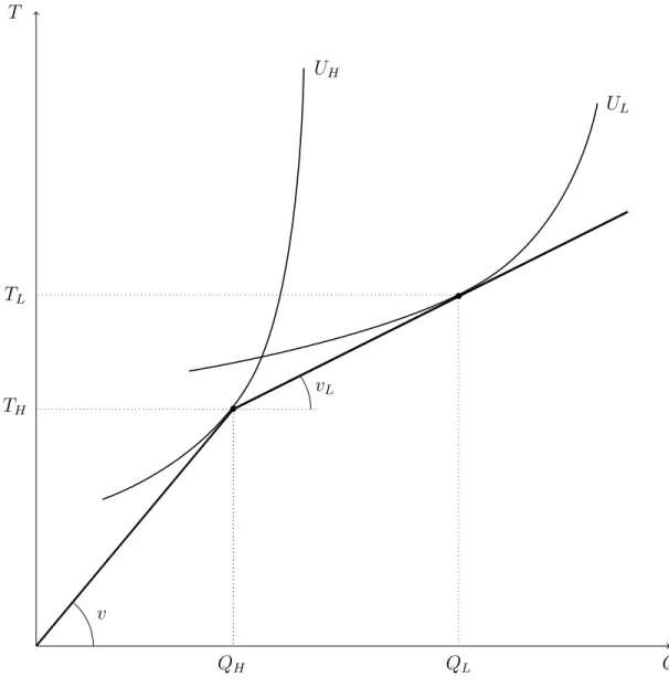
outcomes that have been emphasized in the literature: first, pooling outcomes such as the one described in Attar, Mariotti, and Salani´e (2011), in which both types would trade the same nonzero quantity at a price equal to the average quality of the good; second, separating outcomes such as the one described by Jaynes (1978), Hellwig (1988), and Glosten (1994), and illustrated on Figure 1 below. If one leaves aside the case in which both types trade nonzero quantities on opposite sides of the market, the remaining possibilities for equilibrium outcomes are either that there is no trade in the aggregate, or that only one type actively trades at a fair price in the aggregate.
To illustrate the logic of the no-cross-subsidization result, consider a candidate separating equilibrium with positive quantities QL > QH > 0, as illustrated on Figure 1. The basic
price structure of such an equilibrium is delineated in Lemma 2(ii). —Insert Figure 1 Here—
Let k be a buyer whose profit bk
H from trading with type H is positive. According to
Lemma 4, the aggregate trade (QH, TH) remains available if buyer k removes his menu offer.
He can thus attempt to pivot on (QH, TH) to attract type L, which amounts to offer a
contract ck
L = (QL− QH, TL − TH + εL), for some positive number εL. When εL is small
enough, the loss for buyer k from trading ck
L with type L is negligible, as the slope of the
line segment connecting (QH, TH) and (QL, TL) is the fair price vL. For buyer k’s deviation
to be profitable, he must make a profit when trading with type H. To do so, he can offer an additional contract ck
H = (qHk, tkH + εH), for some positive number εH. Because (qkH, tkH) was
available for trade in equilibrium, ck
L is more attractive than ckH for type L as long as εL is
large enough relative to εH. Now, if type H trades ckH, the deviation is profitable, because,
when εH is small enough, ckH yields a profit close to bkH > 0 when traded by type H, whereas
the loss from trading ck
L with type L is negligible. If type H trades ckL instead, the deviation
is still profitable, because ck
L yields a positive profit when traded by both types. This shows
that there exists no separating equilibrium with positive quantities. The reasoning for a pooling equilibrium is slightly more involved, but reaches the same conclusion.
Remark. The proof of Proposition 3 shows that cross-subsidies are not sustainable in equilibrium because it would otherwise be possible for some buyer to neutralize the type on which he makes a loss by proposing her to mimic the behavior of the other type when facing the other buyers. A key feature of this deviation is that it is performed by a buyer who is actively and profitably trading with one type in equilibrium.17 Moreover, it is crucial for the
argument that this buyer deviates to a menu including two nontrivial contracts targeted at the two types of the seller. Observe that this class of deviations was not considered in the early contributions of Jaynes (1978) and Glosten (1994). Jaynes (1978), who studies strategic competition between insurance providers under nonexclusivity, indeed restricts firms to use simple insurance policies. That is, each firm can propose at most one contract different from the no-trade contract.18 As a consequence, an incumbent firm cannot profitably deviate
by simultaneously making a loss when trading with the high-risk agent and compensating this loss when trading with the low-risk agent. Glosten (1994) characterizes an aggregate
17It is unclear that an entrant would be able to upset the above candidate equilibrium. One might think that an entrant could successfully attempt to nearly reap the aggregate profit on type H, say by proposing a contract of the form (QH, TH+ εH), while making limited losses on type L by proposing a contract of
the form (QL− QH, TL− TH+ εL) as above. Yet this would overlook the fact that by proposing such a
contract to type H, the entrant would globally modify the structure of available trades, unlike the local deviation (qk
H, tkH+ εH) we used in the proof of Proposition 3. As a result, type L might well be attracted
by the contract (QH, TH+ εH) that she may find it profitable to trade along some contracts offered by the
incumbents, thereby upsetting the attempt at a successful entry.
price-quantity schedule that is robust to entry. In our setting, this schedule would be as depicted on Figure 1. By contrast, we do not take the aggregate price-quantity schedule as given, but we derive it from the individual menus offered by the buyers.
So far, we have focused on the aggregate equilibrium implications of our model. We now briefly sketch a few implications for individual equilibrium trades. The following result shows that each traded contract yields zero profit, and that aggregate and individual equilibrium trades have the same sign.
Proposition 4 In any equilibrium, bk
j = 0 and qkL≥ 0 ≥ qkH for all j and k.
Proposition 4 reinforces the basic insight of our model, according to which, in equilibrium, the seller can signal her type only through the sign of the quantities she trades. It follows that if a type does not trade in the aggregate, then she does not trade at all. Hence a pooling equilibrium, when it exists, is actually a no-trade equilibrium.
3.5
Aggregate Equilibrium Trades
In this section, we fully characterize the candidate aggregate equilibrium trades, and we provide necessary conditions for the existence of an equilibrium. Given the price structure of equilibria delineated in Section 3.3 and the no-cross-subsidization result established in Section 3.4, all that remains to be done is to give restrictions on each type’s equilibrium marginal rate of substitution. Two cases need to be distinguished, according to whether or not a type’s aggregate trade is zero in equilibrium.
Our first result is that if type j does not trade in the aggregate, then her equilibrium marginal rate of substitution must lie between v and vj. This is why an equilibrium may fail
to exist for some parameter values.
Lemma 5 If in equilibrium Qj = 0, then vj− τj(0, 0) and τj(0, 0) − v have the same sign.
The intuition for Lemma 5 is as follows. Suppose for instance that QH = 0. If vH >
τH(0, 0), then any buyer could attract type H by proposing a contract offering to buy a small
positive quantity at a unit price lower than vH. For this deviation not to be profitable, type
L must also trade this contract, and one must have τH(0, 0) ≥ v, so that the deviator makes
a loss when both types trade this contract. The same reasoning applies if vH < τH(0, 0), by
considering a contract offering to sell a small positive quantity at a unit price higher than
Our second result is that if type i trades a nonzero quantity in the aggregate, then she must trade efficiently in equilibrium.
Lemma 6 If in equilibrium Qi 6= 0, then τi(Qi, Ti) = vi.
The intuition for Lemma 6 is as follows. Suppose for instance that QL > 0. As
cross-subsidization cannot occur in equilibrium, TL = vLQL. If type L were trading inefficiently in
equilibrium, that is, if τL(QL, TL) 6= vL, then there would exist a contract offering to buy a
positive quantity at a unit price lower than vL, and that would give type L a strictly higher
utility than (QL, TL). Any of the buyers could profitably attract type L by proposing this
contract, which would be even more profitable for the deviating buyer if traded by type H. Hence type L must trade efficiently in equilibrium. The case QH < 0 can be handled in a
symmetric way.
To state our characterization result, it is necessary to define first-best quantities. The following assumption ensures that these quantities are well defined.
Assumption FB For each i, there exists Q∗
i such that τi(Q∗i, viQ∗i) = vi.
Assumption FB states that Q∗
i is the efficient quantity for type i to trade at a unit price
vi that gives an aggregate zero profit for the buyers. An important consequence of the strict
quasiconcavity of ui is that Q∗i ≥ 0 if and only if τi(0, 0) ≤ vi, and that Q∗i = 0 if and only
if τi(0, 0) = vi. In the pure-trade model, Q∗i is defined by c0i(Q∗i) = vi. In the insurance
model, because of the agent’s risk aversion, efficiency requires full insurance for each agent
i, so that Q∗
i = WG− WB. The credit model is special in that the constraint that quantities
must remain nonnegative may be binding. Efficiency requires that the net present value of the project, πifi(T ) − T , be maximized; if this leads to a positive and finite investment, the
promised repayment Q∗
i that makes the investors just break even satisfies πifi0(πiQ∗i) = 1.
By contrast, if πifi0(0) ≤ 1, borrower i’s investment project has a nonpositive net present
value, and it is efficient not to invest in her project. We can now state our main characterization result.
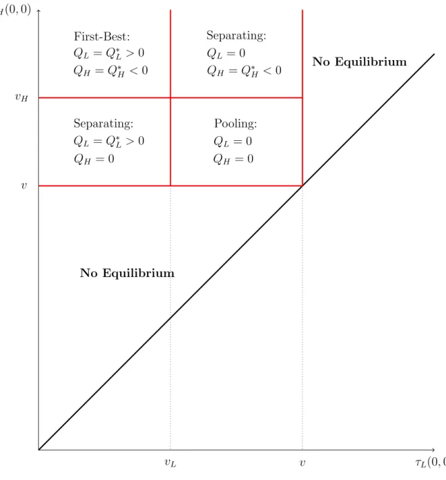
Theorem 1 If an equilibrium exists, then τL(0, 0) ≤ v ≤ τH(0, 0). Moreover,
• If vL≤ τL(0, 0) ≤ v ≤ τH(0, 0) ≤ vH, all equilibria are pooling, with QL= QH = 0.
• Otherwise, all equilibria are separating, and