HAL Id: halshs-00707451
https://halshs.archives-ouvertes.fr/halshs-00707451
Submitted on 12 Jun 2012HAL is a multi-disciplinary open access archive for the deposit and dissemination of sci-entific research documents, whether they are pub-lished or not. The documents may come from
L’archive ouverte pluridisciplinaire HAL, est destinée au dépôt et à la diffusion de documents scientifiques de niveau recherche, publiés ou non, émanant des établissements d’enseignement et de
The user cost of natural resources and the optimal
exploitation of two non-renewable polluting resources
Antoine d’Autume
To cite this version:
Antoine d’Autume. The user cost of natural resources and the optimal exploitation of two non-renewable polluting resources. 2012. �halshs-00707451�
Documents de Travail du
Centre d’Economie de la Sorbonne
The user cost of natural resources and the optimal exploitation of two non-renewable polluting resources
Antoine d’AUTUME
The user cost of natural resources and the optimal exploitation of two non-renewable polluting resources
Antoine d’Autume
Paris School of Economics, Université Paris 1 Panthéon-Sorbonne May 4, 2012
Abstract
We study the optimal extraction of two non-renewable resources when ex-traction costs depend on cumulative previous exex-traction. Defining a complete user cost of natural resources, including environmental damages, allows us to greatly simplify the resolution. It allows us to describe, in a first stage, poten-tial optimal extraction paths of the two resources. It also reduces the problem to one with a unique stock variable, which can easily be solved through time elimination. We also caracterize the evolution of the carbon-price and firm rents.
This framework is applied to a study of oil and coal optimal extraction. The extraction cost of oil is initially lower than the one of coal, but it increases more rapidly with extraction. In a business as usual scenario, without taking into account environmental costs, the optimal path is to use only oil in a first time phase, before using simultaneously the two resources in a second phase, until the backstop becomes profitable. As coal becomes cheaper to extract, it provides for the largest part of extraction in the second time phase.
When the carbon price is taken into account, through a tax or emission permits, the optimal path relies much less on the more polluting coal, prices are higher and the backstop is reached much earlier.
If the backstop price is very high, extraction lasts much longer and it is possible that it becomes optimal to revert to the less polluting oil only in a third time phase.
We consider a model of optimal extraction of two non-renewable polluting resources with a renewable non-polluting backstop1. As in Heal[1976] we
make the realistic assumption that unit extraction costs increase with the cumulative amount of the resource which has already been extracted, as extraction becomes more and more difficult. Extraction of the resource will stop not when it is exhausted but rather when extraction costs become too high. This set-up makes more sense than the original Hotelling set-up where the overall quantity of the resource is given and can be extracted at a zero or possibly constant unit cost. In the Hotelling setting the resource scarcity is absolute and the only problem is when to consume the existing quantity. In the setting we adopt, scarcity is economic, which appears much more satisfactory. Extraction will stop when it becomes too costly in comparison to other non-renewable resources as well as renewable backstops presently too costly to be used. Oil for instance will not cease to be used when resources will be exhausted but when the high level of extracting costs will choke extraction. As Sheikh Yamani famously said, "the Stone Age did not end for lack of stone". More concretely the level of exploitable oil resources has been constantly reevaluated upward as new discoveries were made but also, and more and more, as higher extraction costs became acceptable.
Heal’s approach has been followed by Hanson[1980] and more recently, Hoel[2011], Bureau[2008], Van der Ploeg and Withagen[2011] and others
Our first aim, in this paper, is to put forward a new and synthetic in-terpretation of the intertemporal trade-offs faced by economic agents when using natural resources. To this end, we define a complete user cost of nat-ural resources. This notion is standard in the case of physical capital. If K is capital, δ the physical rate of depreciation and I = ˙K + δK the investment flow, the user cost of capital is (r + δ)K, including the physical cost of depre-ciation and the interest charge of holding an amount K of capital. The user cost is the true cost of using capital and allows to define instantaneous profit in a meaningful way. The total cost of using capital over time may then be represented alternatively by the discounted value of investment flows or by the discounted value of user costs. The equivalence between these two mea-sures follows from pure accounting and, more specifically, by an integration by parts of the discounted integral of profits.
We define in a similar way the complete user cost of natural resources. Its first component is the true measure of the extraction costs currently supported. It takes the form of an interest charge on cumulative extraction costs. A second component of the cost is environmental, as the use of fossil
1I acknowledge the support of the French National Research Agency (ANR) under the
fuels generates greenhouse gas emissions which contribute to global warming. It takes the usual form of a damage function.
To our knowledge, the notion of an user cost of natural resources has not been stated explicitely in the literature. It appears implicitely in Van der Ploeg and Withagen[2011]2 but the corresponding equation is derived
from optimality conditions, rather than from an a priori reformulation of the problem in terms of complete user costs. On the other hand, the integration by parts which leads to this reformulation appears in a number of articles on renewable or non renewable resources: see Spence-Starett[1975], who developed a general analysis of models where the Hamiltonian is linear with respect to the control variable and studied most rapid paths converging to a singular solution; see also Leonard-Long[1992], who use it in various contexts. But again no general presentation of the user cost and its importance is offered. In d’Autume[2012], we also use the user cost of natural resources to study the optimal behavior of an extracting firm, that is a model where the Hamiltonian is linear with respect to the extraction rate.
The definition of complete user costs provides an intuitive and simple method to characterize the optimal extraction path of two non-renewable resources, say oil and coal. This issue has been examined in numerous articles and in particular in recent papers by Van der Ploeg and Withagen[2011] and Chakravorty, Moreaux and Tidball[2008]. Both articles stress a possible energy reversal, that is a return to a resource which had earlier been forsaken, a phenomenon which may also appear in our own setting. Our framework is close to the one of Van der Ploeg and Withagen[2011], but we treat the case of two non-renewable resources whereas they treat, for simplification, the second resource, coal, as a dirty renewable backstop. Our framework differs more markedly from the one used in Chakravorty, Moreaux and Tidball[2008]. On one hand, they do not introduce extraction costs increasing with the quantity already extracted. On the other hand, we do not take into account natural emission absorption, which is admittedly a limitation of our approach.
Our approach allows us to characterize, in a first stage, possible extrac-tion paths, before studying optimal dynamics. We then reduce the dynamic system to one state variable, namely total resource extraction.
Two different typical configurations appear. In the first one, the economy begins to exploit the less costly resource and after some time switches to a second regime where both resource are simultaneously extracted. During this second time phase, the economy follows an iso-"user cost" curve, and does so until the moment where the two costs simultaneously reach the cost of the backstop, say solar energy. In the second configuration, it proves impossible
to follow the iso-cost after some point, as this would require that the extracted stock of one of the resource decrease, which is impossible by definition. We then face an irreversibility problem akin to the one considered by Arrow-Kurz[1970] in the case of physical investment and the solution method is similar to the one they proposed. We may then observe an energy reversal. The economy may revert to a regime where one resource, the less polluting one, is the sole to be extracted.
We use our framework to simulate the ordering of oil and coal extraction. The extraction cost of oil is initially lower than the one of coal, but it increases more rapidly with extraction. In a business as usual scenario, without taking into account environmental costs, the optimal path is to use only oil in a first time phase, before using simultaneously the two resources in a second phase, until the backstop becomes profitable. As coal becomes cheaper to extract, it provides for the largest part of extraction in the second time phase.
When the carbon price is taken into account, through a tax or emission permits, the optimal path relies much less on the more polluting coal, prices are higher and the backstop is reached much earlier. It may be the case that the economy has to revert to an oil only regime if the polluting power of oil is large.
1
The framework
The two resources and the backstop are perfectly substitutable in consump-tion. Let q1, q2 and x be the consumption levels of the three goods. Current
utility is an increasing and concave function of total consumption: U (q1+ q2+ x).
The resources differ by their extraction costs as well as by their polluting character.
For i = 1, 2, we denote at time t by qi,t and Zi,t the flow of extraction of
resource i and the cumulated sum of past extractions, with an arbitrary and unspecified initial point. Thus,
˙
Zi,t = qi,t. (1)
As in Heal[1976], the unit extraction cost of resource i is an increasing, differentiable and convex function Gi(Zi). This unit cost does not depend
on the flow qi currently extracted.
Extraction also has a detrimental environmental impact. More specifi-cally, the two resources are fossil fuels the consumption of which generates
GreenHouse Gases emissions which contribute to global warming. We do not take into account the natural absorption of GreenHouse Gases by the envi-ronment and simply assume that the stock of pollutants created by the use of resource i is proportional to the stock already extracted,
Ei = φiZi
with a positive emission coefficient φi of resource i. This implies3 E˙
i = φiqi.
Current environmental damages are then defined as
D (φ1Z1+ φ2Z2) ,
where D is an increasing, differentiable and convex function.
Lastly, we denote by pbthe constant unit production cost of the backstop.
Under these assumptions, the social welfare takes the following form, where r is rate of discount, identical in this framework to the consumers rate of time preference4:
Z ∞
0
e−rt[U (q1 + q2+ x)− pbx− G1(Z1) q1− G (Z2) q2− D (φ1Z1+ φ2Z2)] dt.
(2)
2
The complete user cost of natural resources
We now introduce a user cost of natural resources.
For a moment, we consider a unique resource. Assuming that the unit extraction cost does not depend on the quantity currently extracted implies that the time required to extract a given quantity, or indeed the time profile of extraction, does not affect the overall cost of extraction. Starting at time T1 from an extraction level ZT1 and extracting between T1 and T2 a flow qt, the integral of wich is ZT2 has the following cost
Z T2 T1 G(Zt)qtdt = Z ZT2 ZT1 G(z)dz = H(ZT2)− H (ZT1) (3)
3More generally, we might assume that the pollution stock associated with a resource
is an increasing and convex function Ei = fi(Zi) of cumulative extraction. This would
imply ˙Ei = fi0(Zi) qi, so that the emission coefficient of new extraction of resource i would
be an increasing of Zi. The pollution associated with extraction would then increase over
time as extraction becomes more and more difficult.
It does not depend on the time profile of extraction
The economic total cost of course does depend on this profile, as it in-corporates interest charges. For generality, let us consider a time varying discount rate rt and define Rt =
Rt
0 rsds. A simple integration by parts
yields5 Z T2 T1 e−RtG (Z t) qtdt = e−RT2H (ZT2)− e −RT1H (Z T1) + Z T2 T1 e−Rtr tH (Zt) dt (4) The total economic cost now includes the integral of rtH (Zt). As
men-tioned in the introduction, this relation is similar to the one which applies in the case of physical investment. Let Kt be the stock of capital, δ its rate
of depreciation and It = ˙Kt+ δKtgross investment. A similar integration by
parts yields: Z T2 T1 e−RtI tdt = e−RT2KT2 − e −RT1K T1 + Z T2 T1 e−Rt(r t+ δ) Ktdt
rtH (Zt) thus appears as the user cost of the resource stock, as (rt+ δ) Kt
is the user cost of physical capital. In the simple capital model we consider, one unit of capital is produced with one unit of generic good, so that K is the cumulative cost which has to be supported to reach a capital level equal to K. In the resource model, H(Z) is the cumulative cost which has to be supported to reach a resource level Z6.
In our setting with two polluting non-renewable resources, this leads us to the following definition and proposition7.
Definition 1 The complete user cost of natural resources is
Γ(Z1, Z2) = rH1(Z1) + rH2(Z2) + D (φ1Z1+ φ2Z2) (5)
Marginal complete user costs are the derivatives
Γi(Z1, Z2) = rGi(Zi) + φiD0(φ1Z1+ φ2Z2) , i = 1, 2 (6)
5This detailed in appendix 1.
6The two models differ regarding the utility side. In the physical capital model, utility
derives from the production made with the capital stock, so that K has a positive so-cial value. In the resource model, utility derives from consuming the flow of extraction. Moreover Z has a negative social value, as a higher Z means higher marginal extraction costs.
Proposition 2 Up to initial constants, social welfare is equal to
Z ∞
0
e−rt[U (q1+ q2+ x)− pbx− Γ(Z1, Z2)] dt (7)
The complete user cost of natural resources Γ(Z1, Z2) is the sum of the
user cost of extraction and the environmental damage caused by emissions. Social welfare may be expressed as the discounted value of the differ-ence between the utility derived from consuming natural resources and their complete user cost.
We also define the two marginal complete user costs. As environmental damages depend on the two stocks Z1 and Z2, the two marginal user costs
are linked and each one depends on the two stocks.
3
The ordering of the two resources
extrac-tion
Knowledge of the user costs is sufficient to characterize possible orderings of extraction of the resources.
Z 1 min Γ1 Γ2 Z 1, Z2
Figure 1: Extraction costs
3.1
The case without pollution
Let us first consider the case without pollution. marginal user costs are simply rG1(Z1) and rG2(Z2).
As the two resources as well as the backstop are perfectly substitutable in consumption, they can only be produced simultaneously if they have the same price. The price of a resource is not equal to its cost, as it includes a
O I B Z 1 Z 2 G 1 = pb G 2 = G1 G2 = pb
Figure 2: Extraction path 1
O I B Z 1 Z 2 G1 = pb G2 = G1 G 2 = pb
Figure 3: Extraction path 2
scarcity rent. As we shall see8, however, the equality of prices over a time
interval is only possible if user costs are equal.
Without pollution, this reduces to the condition that current extraction costs be equal:
G1(Z1) = G2(Z2) .
Let us consider the case of figure (1). Resource 1 is initially less costly to extract than resource 2, but its cost increases more steeply. The two resources may be extracted simultaneously only if cumulative extraction of resource 1 has reached the minimum level Zmin
1 such that G1 ¡ Zmin 1 ¢ = G2(0). Figure
(2) plots the equal cost locus in the plane (Z1, Z2). As each cost increases
with its cumulative extraction level, the locus has a positive slope dZ2/dZ1 =
G0
1(Z1) /G02(Z2). At each point located above or to the left of the curve, the
extraction cost of the first resource is lower than the one of resource 2 and marginal user costs rG1 and rG2 are ranked in the same way.
The economy switches to the backstop at point B on the figure, when both
B Z Z 2 Γ1 = p b Γ 2 = pb Γ 2 = Γ1 A O
Figure 4: Forsaking resource 2
extraction costs reach the price pbof the backstop9. The vertical and
horizon-tal lines through B are respectively the loci G1(Z1) = pb and G2(Z2) = pb.
The optimal path is intuitive. Remember than Z1and Z2cannot decrease.
Assume for exemple that the initial amounts already extracted correspond to point O on figure (2). The initial user cost of resource 2 is higher than the one of resource 1. It is optimal to extract only resource 1. As it is exploited, the user cost of resource 1 increases. The economy moves on segment OI until the two resources costs are equalized. The economy then starts extracting simultaneously the two resources, at such rates that the two costs remain equal. The economy moves on the curved segment IB.
The shares of the two resources may be read on the diagram. We have q2/q1 = ˙Z2/ ˙Z1 = dZ2/dZ1 = G01(Z1) /G02(Z2) which, as we have seen, is the
slope of the equal cost curve. This slope, i.e. the relative share of resource 2 extraction, decreases as exploitation goes on.
During this time period the price of energy increases until it reaches the price of the backstop. Extraction then has to stop. The economy switches to consumption of the backstop and the price of energy remains later on equal to pb. Rents disappear so that the extraction costs are equal to the price of
the backstop.
Figure (3) considers the opposite case of a relatively high initial level of Z1. The initial extraction cost of resource 1 is larger than the one of resource
2 so that the economy first uses resource 2 only and moves on a vertical straight line10 until it reaches the iso-cost curve.
9As Γ
i is a user cost, it cannot be compared to the price of the backstop. The relevant
comparison is between the discounted value of future user costs, which reduces here to
Γi/r = Gi and pb.
10Other cases would be the ones of initial very high levels of Z
1 or Z2. The economy
We thus have been able to characterize intuitively the extraction path of the two resources. The formal dynamic analysis will only determine the speed at which this path will be followed and, of course, confirm our intuitive results.
3.2
The case with pollution
We now consider the general case with environmental damages.
We again define the equal cost curve Γ1(Z1, Z2) = Γ2(Z1, Z2) curve in the
(Z1, Z2) plane. If this curve always has a positive slope, not much is changed.
The optimal ordering of exploitation of the two resources follows the same principles than in the previous case. 11.
A second configuration arises when the iso-cost curve reaches a maximum, as in the case of figure (4). As Z2 cannot decrease, the economy cannot go on
following this curve. It ceases at some point to exploit resource 2 and engages on the horizontal segment AB until the moment when the cost of extracting resource 1 reaches the cost of the backstop.
For reasons which will be explained later, the economy does not reach the maximum of the curve and forsakes extraction of resource 2 before reaching it. The situation is one of irreversibility, as the Zis cannot decrease, and is
reminiscent of the Arrow-Kurz[1970] analysis of irreversible physical invest-ment.
The optimal switch point is endogenous. In this more complicated case, the optimal ordering of extraction cannot be determined ex ante, without solving the dynamic model. It depends on all the elements of the model and, in particular, on the utility function, that is on the demand side.
Let us now clarify the shape of the iso-cost curve. We may show that the case of forsaking one resource only occurs if this resource is more polluting than the other one, and sufficiently so.
The slope of the curve is now dZ2 dZ1 ¯ ¯ ¯ ¯ Γ2=Γ1 = Γ11− Γ21 Γ22− Γ12 (8) From (6), Γ11= G01+ (φ21/r)D00> 0 Γ22= G02+ (φ22/r)D00> 0 Γ12 = Γ21 = (φ1φ2/r)D00 > 0
vertical straight line until it switches to the backstop. If both initial Z1and Z2 were very
high, the economy would of course switch at once to the backstop.
11One difference is that the Γ
Γ11− Γ21 = G01+ (φ1− φ2) (φ1/r)D00
Γ22− Γ12 = G02+ (φ2− φ1) (φ2/r)D00
Assume resource 2 to pollute more, so that φ2 > φ1. The denominator of slope (8) is always positive, while the numerator may become negative, in particular when D00 is high that is when total emissions become high. The
iso-cost curve then reaches a maximum and the economy forsakes extraction of the polluting resource at some point before reaching the maximum12.
The previous derivatives also allow to calculate the slopes of the curves describing the switch to the backstop :
dZ2 dZ1 ¯ ¯ ¯ ¯ Γ1=pb =−Γ11 Γ12 , dZ2 dZ1 ¯ ¯ ¯ ¯ Γ2=pb =−Γ21 Γ22 .
Both are negative. In the more natural case, the cross terms are smaller which implies that the Γ1/r = pb curve is steeper than the Γ2/r = pb curve.
4
The dynamic analysis
4.1
Optimality conditions
The problem is to maximize social welfare (7) under the resource constraints. Z ∞ 0 e−rt[U (q1+ q2+ x)− pbx− Γ (Z1, Z2)] dt ˙ Z1 = q1 ≥ 0, Z˙2 = q2 ≥ 0 Z1,0 and Z2,0 given.
Let pi, i = 1, 2 be the shadow prices of the two resource constraints.
Proposition 3 First order Conditions are the following
x≥ 0, U0(q
1+ q2+ x)− pb ≤ 0 (9)
qi ≥ 0, U0(q1+ q2+ x)− pi ≤ 0, i = 1, 2 (10)
˙pi = rpi− Γi(Z1, Z2) , i = 1, 2 (11)
with slackness conditions for the static conditions.
The proof is not reproduced.
4.2
Resources prices, the carbon price and rents
Equation (11) states that the shadow price of a resource is the discounted value of its future complete marginal user costs.This relation extends the Hotelling rule to the case of endogenous extraction costs and environmental costs. As the complete user cost is non decreasing, its discounted cumulative value, namely the price, is also non decreasing.
Condition may also be written as a no arbitrage condition
r = Γi(Z1, Z2) pi + ˙pi pi = φiD 0 pi +rGi(Z1, Z2) pi + ˙pi pi . (12)
Distinguishing the two components of the marginal user cost leads to distinguish two components in the price of a resource.
The first one is the discounted value of the marginal environmental dam-ages it generates. It is the product of the emission coefficient φi and the carbon price τ , defined as the discounted value of future marginal environ-mental damages:
˙τ = rτ − D0 (13)
The second part, say p2
i, is the discounted value of marginal extraction
user costs: ˙p2i = rp2i − rGi which yields p2it = Z ∞ t e−r(s−t)rGisds.
An integration by parts yields13
p2it= Git+ Z ∞ t e−r(s−t)G˙isds def = Git+ ψit with ˙ψi = rψi− ˙Gi (14)
ψiis the discounted value of future extraction cost increases. As the
analy-sis of the competitive extraction firm behavior14 would show, it is the
pro-ducer rent gained by the resource field owner. This rent reflects the scarcity of the resource in the sense that extraction will become more and more costly. It may increase with time, but will ultimately decrease and become zero when the exploitation of the resource ceases.
13Letting u = G
is, dv = e−r(s−t)rds, du = ˙Gis, v =−e−r(s−t) and taking into account
the fact that Gis will remain constant after the backstop starts to be used.
Proposition 4 The price of a resource
pi = Gi+ φiτ + ψi (15)
is the sum of current marginal extraction cost, the carbon value of emissions and the producer rent.
The carbon price is the discounted sum of future marginal environmental damages, while the producer rent is the discounted value of future extraction cost increases.
The price thus appears as the sum of the current extraction cost and the discounted sum of all marginal damages inflicted by current extraction to natural capital and the environment. Extraction reduces future extraction possibilities and thus the value of natural capital. Extraction also leads to emissions which affect the environment and reduce its value.
In a competitive market economy the first element takes the form of a rent gained by the owner of the resource field. The second element is the cost of carbon emissions, which has to be internalized through a carbon-tax or a market for emission permits.
4.3
The dynamics of aggregate resources and the two
regimes
As resources are perfectly substitutable we may define the total amount of already extracted resources and the total extraction flow
Z = Z1+ Z2 (16)
q = q1+ q2 = ˙Z (17)
We also define the demand function qd(p) as the inverse function of
mar-ginal utility.
Two types of regimes are possible depending on which resources are cur-rently extracted.
Proposition 5 The regime with joint extraction of the two resources, q1 >
0, q2 > 0, is characterized as follows.
i) The two resources have the same price and the backstop is unused :
U0(q) = p < p
ii) They have the same complete user cost:
Γ1(Z1, Z2) = Γ2(Z1, Z2) (19)
This cost can be expressed as a function Γ(Z) of total cumulative extrac-tion.
iii) Cumulative extraction levels and extraction flows may be expressed as functions of total cumulative extraction and the total extraction flow:
Z1 = ψ1(Z), Z2 = ψ2(Z)
q1 = ψ01(Z)q, Z2 = ψ02(Z)q
iv) The dynamics in this regime is described by the following system:
˙
Z = qd(p) (20)
˙p = rp− Γ (Z) (21)
v) Eliminating time reduces the dynamics to the unique differential equa-tion
p0(Z) = rp(Z)− Γ(Z)
qd(p(Z)) , (22)
The two resources can obviously be simultaneously exploited if and only if they have the same price, which has to be smaller than the price of the backstop, in order to make production of the latter unprofitable.
From conditions (11) describing price evolutions, the two prices may be equal for a finite time period only if both complete costs are equal15. Note
that prices are not equal to costs as implicit rents are present, but these rents have to be equal.
From (19) and (16) we derive the shares of cumulative extractions Zi =
ψi(Z), as well as the shares of current extraction rates qi = ˙Zi = ψ0i(Z) ˙Z =
ψ0 i(Z) q.
We thus are led to a model with only one stock. Resolution is also sim-plified by the fact that the terminal point is not be a saddle-point and will be reached in finite time. This allows us to eliminate time and use a one dimensional differential equation in the (Z, p) plane.
We have
˙p/ ˙Z = (dp/dt) / (dZ/dt) = dp/dZ = p0(Z),
and ˙Z = qd(p). Using (11), and the equality of prices and costs, we are led
to differential equation (22).
Let us now consider the regime with extraction of the first resource only. Cumulative extraction of the second resource remains constant at level ¯Z2
and we have
Z = Z1+ ¯Z2
q = q1 > 0, q2 = 0
Proposition 6 The regime with extraction of the sole resource one is char-acterized as follows
i) Prices and extraction flows are such that
U0(q
1) = p1 < min[p2, pb]
ii) The dynamics is
˙ Z = qd(p1) ˙p1 = rp1− Γ1 ¡ Z − ¯Z2, ¯Z2 ¢ .
iii) Eliminating time yields
p0 1(Z) = rp1(Z)− Γ1 ¡ Z− ¯Z2, ¯Z2 ¢ qd(p 1(Z)) (23)
iv) The price of resource 2 varies according to
p0 2(Z) = rp2(Z)− Γ2 ¡ Z − ¯Z2, ¯Z2 ¢ qd(p∗ 1(Z)) (24) where p∗
1(Z) is the solution of (23), with an appropriate boundary condition.
The price of the sole resource which is extracted is smaller than the prices of the two competing energy sources, which makes their use non-profitable. As we shall see, this does not require the complete user cost of the extracted resource to be lower than the one of the second resource, as the two rents are not equal.
These propositions validate our previous intuitive analysis of possible ex-traction paths. The cost relations we described in section 3, and in particular the equality of the two complete user costs of two resources when they are simultaneously extracted are simply necessary conditions of the minimization of the discounted total cost of producing a given flow of resource q1t+q2t+xt,
for 0 ≤ t < ∞. The maximization of social welfare clearly requires this min-imization and it is easy to check that the description of the regimes follows from this second and simpler problem.
4.4
Global resolution in the case of an ever increasing
iso-cost curve
Let us consider a case, with pollution, where the iso-cost curve in the plane (Z1, Z2) is always increasing up to the backstop point. The configuration
is similar to the one in figure (2) but environmental damages are now part of the problem. The iso-cost curve is represented by a function Z2∗(Z1). We
assume the initial point (Z1,0, Z2,0) to be such that Γ2 > Γ1, as in figure (2) .
The solution is of the following type:
- first, a regime with resource 1 only extracted; - second, a regime with the two resources extracted. The model can be solved by simple backward recursion.
The terminal point is the switch point to the backstop. Cumulative ex-traction is ZB such that Γ(ZB)/r = p
b and the price level is p
¡
ZB¢= p b.
The dynamics in the regime with the two resources extracted is deter-mined by differential equation (22) with terminal condition p¡ZB¢ = p
b.
The switch point ¡Z1I, Z2I
¢
between this regime and the first one with only resource 1 extracted is determined by ZI
2 = Z2,0 = Z2∗(Z1I) and we have
ZI = ZI
1 + Z2,0 . The price p(ZI) is known from the dynamics of the second
regime.
The dynamics of the first regime is determined by (23) with a known p(ZI) as terminal condition.
This completes the determination of the optimal solution p∗(Z), for all
Z ∈£Z0, ZB
¤ .
It remains to check that this solution satisfies p2 > p1 at all point on
the first regime trajectory, where Z2 = Z2,0. Price p∗2(Z) is then solution to
equation (24), with terminal condition p2(ZI) = p∗(ZI).
Let ∆p = p∗2(Z)− p∗(Z) and ∆Γ = Γ
2(Z− Z2,0, Z2,0)− Γ1(Z− Z2,0, Z2,0).
∆p satisfies equation
∆p0(Z) = r∆p(Z)− ∆Γ(Z − Z2,0, Z2,0)
qd(p∗(Z)) (25)
In the time dependent equivalent equation, ∆p is the discounted value of future ∆Γ up to ZA at which point it is zero. As ∆Γ is positive for all Z
between Z0 and ZA, ∆p is positive on this interval, as it should to prevent
extraction of resource 2.
The optimal trajectory p∗(Z) is thus determined for all Z ∈ £Z 0, ZB
¤ . The evolution of p as a function of time then follows from the resolution of differential equation
˙
traj 1 optimal traj 3 Z1A Z2A Z1B 150 200 250 300 Z1 40 45 50 55 Z2
Figure 5: Possible solutions
The evolution of all other variables follows.
4.5
The resolution in the case of an iso-cost curve with
a maximum
Let us now consider the case of figure (4). The point where the two user costs, divided by r, simultaneously reach the cost of the backstop is now over the maximum of the iso-cost curve, in its decreasing section.
We now face an irreversibility problem as cumulative extraction Z2cannot
be decreasing. The optimal solution ends with a phase where only resource 2 is extracted, following the phase where the two resources are jointly extracted.
Consider figure (5). The problem is to determine the point ¡ZA 1, Z2A
¢ where the trajectory leaves the upward sloping iso-cost curve to engage in an horizontal trajectory. The figure identifies two possible solutions.
i) Point ¡ZA 1 , Z2A
¢
is at the maximum of the iso-cost curve. The path followed in the final "resource one only" regime would lie completely in the Γ2 > Γ1 region, that is in a region where ∆Γ = Γ2 − Γ1 > 0. On the other
hand the price gap ∆p = p2− p1 has to be non negative at all points of the
last regime16, in order to forbid the use of resource 2. Following equation
(11) and its interpretation, the price gap is an average of future positive cost gaps. It would be strictly positive at the initial point ZA = ZA
1 + Z2A of the
regime. This is impossible as the price gap has to be zero at any point on the iso-cost curve. This first trajectory is ruled out.
16It is strictly positive at the terminal point where Γ
ii) The initial point ¡ZA 1, Z2A
¢
is such that the economy reaches, at the end of its horizontal trajectory, the point on the iso-cost curve where Γ1/r =
Γ2/r = pb = p1 = p2. A symetric argument rules out this path, as it lies
completely in the ∆Γ < 0 region. ∆p would be strictly negative at the initial point of the regime.
This suggests that the optimal path lies between the previous two paths we just considered. It is indeed possible to find a path, lying alternatively in the ∆Γ < 0 and ∆Γ > 0 regions, such that at the initial point we have ∆p = 0. As we show in the appendix a simple one dimensional loop allows to determine the optimal path.
Note that during the first part of this optimal path, which lies below the iso-cost curve, the complete user cost of resource 2 is lower than the one of resource 1 and yet resource 2 is not extracted. The static comparison of complete user costs is insufficient to determine which resources should currently be exploited.
5
Simulations
We use the following functions
Gi(Zi) = ci+ giZi, D0(E) = δE2/2
Then
Γi(Z1, Z2) = r (ci+ giZi) + φiδ (φ1Z1+ φ2Z2)2/2
The slope of the curve is now dZ2 dZ1 ¯ ¯ ¯ ¯ Γ2=Γ1 = Γ11− Γ21 Γ22− Γ12 = g1− φ1(φ2− φ1) (δ/r) (φ1Z1+ φ2Z2) g2+ φ2(φ2 − φ1) (δ/r) (φ1Z1 + φ2Z2)
We assume a higher emission coefficient for resource 2, coal, than for resource 1, oil, ie φ2 > φ1.
The denominator is always positive. The numerator is positive if the stock φ1Z1+ φ2Z2 of emissions is low but becomes positive when it is larger
than rg
1
δφ1(φ2− φ1)
We thus have the configuration of figure (4), with a possible decreasing part of the iso-cost curve.
The marginal utility is U0(q) = d q−1/ε, which yields the following total
energy demand
q1+ q2+ x = qd(p) = (d/p)ε
Table 1 describes the 2009 oil and coal supplies and the CO2 emissions they generate. We use these data as a benchmark for our rough calibration. To make results more transparent, we express the price of oil in terms of dollars per barrel, in a range of 50/100, while extraction annual flows are expressed in terms of billions of ton of oil equivalent, in a range of 1/5.
The calibration is the following.
c1 = 10, c2 = 25, g1 = 1/3, g2 = 1/6, φ1 = 1, φ2 = 1.5
r = .02, ε = .1, d = 4 107, δ = 2.2 10−5
Z10= 0, Z20 = 30.
Coal induces 50% more CO2 emissions than oil. Coefficient δ describes the weight of the environmental cost in the complete cost of the resources. It is choosen so that the environmental cost of oil is equal to 6 when the extraction cost is 30, that is when Z1 = 60 Z2 = 30, Γ1 = 36.
The cost of the backstop is pb = 80.
Tables 2, 3 and 4 and Figures 6, 7 and 8 describe the results of the simulation.
Source : EIA Key World Energy Statistics Table 1
Date 0 oil 1st switch oil/coal 2d switch backstop
Z1 0 60 210 Z2 30 30 330 q1 4.0 3.9/1.3 1.2 q2 0 0/2.6 2.5 p1 41.4 49.2 80 p2 44.2 49.2 80 G1 10 30 80 G2 30 30 80 µ1 31.4 19.2 0 µ2 14.2 19.2 0 time 0 15.3 134.3
Table 2 Business as usual
Date 0 oil 1st switch oil/coal 2d switch bs
Z1 0 71.0 123.6 Z2 30 30 70.9 q1 3.8 3.8/1.9 2.3 q2 0 0/1.9 1.4 p1 56.7 71.1 80 p2 60.0 71.1 80 G1 10 33.7 51.2 G2 30 30 36.8 µ1 29.2 13.7 0 µ2 3.7 5.4 0 φ1τ 17.5 23.8 28.8 φ2τ 26.2 35.7 43.2 time 0 18.7 43.8
Table 3 With environmental damages
Date 0 oil 1st switch oil/coal 2d switch oil 3d switch bs
Z1 0 89.6 160.4 331.3 Z2 30 30 50.0 50.0 q1 3.6 3.5/3.5 2.9 3.3 q2 0 0/1.1 0.4 0 p1 115.6 170.8 230.2 300 p2 120.0 170.8 230.2 302.7 G1 10 39.9 63.5 120.4 G2 30 30 33.3 33.3 µ1 46.7 38.9 35.5 0 µ2 1.6 2.7 0 0 φ1τ 58.8 92.1 131.2 179.6 φ2τ 88.2 138.2 196.8 269.4 time 0 25.5 52.3 104.4
oil coal 50 100 150 200 250 300 Z 20 40 60 80 G1,G2 Cost functions coal oil G1 = pb G2 = pb G1 = G2 50 100 150 200 250 300 350Z1 100 200 300 400 500 600 Z2 Extraction path coal oil coal oil price extraction cost 100 200 300 400 500 z 20 40 60 80 p1,p2,G1,G2
Prices and costs
coal oil 100 200 300 400 500 z 50 100 150 200 250 300 Z1,Z2 Extraction paths oil oil coal coal 100 200 300 400 500 z 1 2 3 4 q1,q2 Extraction rates coal oil oil coal 20 40 60 80 100 120 140t 1 2 3 4 q1,q2
Extraction rates (time)
price extraction cost 20 40 60 80 100 120 140t 20 40 60 80 p1,G12
The price of oil
price extraction cost 20 40 60 80 100 120 140t 20 40 60 80 p2,G2
The price of coal
G1r = pb G2r = pb coal oil 20 40 60 80 100 120 140Z1 20 40 60 80 100 Z2
Figure 1 The extraction path
coal oil business as usual optimal 50 100 150 200 Z1 50 100 150 200 250 300 Z2
Figure 2 Business as usual and optimal extraction paths price user costr coal oil coal oil 50 100 150 200 z 20 40 60 80 p1,p2,G1r,G2r
Figure 3 Prices and complete user costs
oil coal 50 100 150 200 z 20 40 60 80 100 120 Z1,Z2
Figure 4 Extraction paths
oil oil coal coal 50 100 150 200 z 1 2 3 q1,q2
Figure 5 Extraction rates
oil oil coal coal 10 20 30 40 t 1 2 3 q1,q2
Figure 6 Extraction rates (time)
rent carbon price price extraction cost 10 20 30 40 t 20 40 60 80 p1 rent carbon price price extraction cost 10 20 30 40 t 20 40 60 80 p2
G1r = pb G2r = pb coal oil G1 = G2Å 100 200 300 400Z1 20 40 60 80 Z2 optimal optimal oil coal 50 100 150 200 250 300 Z1 10 20 30 40 50 60 Z2 user costr price coal oil coal oil coal oil coal oil oil coalÇ 100 200 300 400 z 50 100 150 200 250 300 p1,p2,G1r,G2r oil coal 100 200 300 400 z 50 100 150 200 250 300 Z1,Z2 oil coal 100 200 300 400 z 0.5 1.0 1.5 2.0 2.5 3.0 3.5 q1,q2 oil coal 20 40 60 80 100 t 0.5 1.0 1.5 2.0 2.5 3.0 3.5 q1,q2 extraction cost price carbon price rent 20 40 60 80 100 t 50 100 150 200 250 300 p1 carbon price price extraction cost 20 40 60 80 100 t 50 100 150 200 250 300 p2
i) Business as usual
We first assume that agents do not take into account environmental costs. The extraction cost of oil is initially lower than the one of coal, but increases more rapidly. After a first regime where oil only is exploited a joint oil-coal regime is sustained until the backstop become profitable when cumulative extractions reach respectively Z1 = 210 and Z2 = 330. In the first phase only
oil is extracted at a level q1 close to 4. In the second phase, oil extraction q1
falls to a leval equal to 1.3 while coal extraction begins at q2 = 2.6. The last
three figures describe evolution as functions of time. As the carbon price is not taken into account, fossil energy prices remain low for a long time and their exploitation lasts for 134 years ! The last two figures describe the two components of the two prices, namely extraction costs and rents. Producer rents reach zero when extraction ceases. Coal rents are much lower than oil rents.
ii) Taking into account carbon prices
We now assume that optimal carbon prices are incorporated into energy prices. The economy thus follows an optimal path. Energy prices are higher and extraction now stops much earlier, when Z1 = 123.6 and Z2 = 70.9, after
43.8 years. Contrary to the business as usual case, the economy relies much less on polluting coal. The last two pictures describe the decomposition of the two energy prices, which now include carbon prices, which leads to lower rents, in particular in the case of oil.
iii) The case of a return to oil
With our calibration, the extraction path in the plane (Z1, Z2) reaches
a maximum when Z1 = 416 and Z2 = 130. The common complete cost of
the two energy is then equal to 353. Thus, if the price of the backstop was higher than this level, the economy would eventually forsake coal extraction and revert to a final phase with oil only extraction.
To make stronger this phenomenon, we modify our calibration and now assume higher environmental damages damages. The weight δ of damages in the utility function is doubled to δ = 4.4 10−5. The backstop prices as assumed to be pb = 300, which corresponds to a point located well after the
maximum of the iso-cost curve.
Coal exploitation is now temporary and takes place between years 25.5 and 52.3. Carbon prices are much higher, which reduces producers rents. The rent of coal producers almost disappears.
6
Appendix 1 Reformulation of Social
Wel-fare
Consider A = Z T2 T1 e−RtG (Z t) qtdtIntegrating by parts with u = e−Rt, dv = G (Z
t) qt, du = −rte−Rtdt, v = H(Zt) yields A =£e−RtH (Z t) ¤T2 T1 + Z T2 T1 e−Rtr tH (Zt) dt
which is relation (4)in the text.
The same reasoning is applied to social welfare (2), where the integral is taken between 0 and infinity. The existence of the backstop prevents Zit
to tend to infinity and ensures that limt→∞e−rtHi(Zit) = 0. Relation (7)
follows.
6.1
Appendix 2 Determination of the optimal solution
in the case of an iso-cost curve with a maximum
Let us choose an arbitrary ZA
1 in the increasing zone of the iso-cost curve
and define (as functions of ZA
1 ) Z2A, ZA, Z1B and ZB such that
Γ1 ¡ Z1A, Z2A¢= Γ2 ¡ Z1A, Z2A¢ Γ1 ¡ ZB 1 , Z2A ¢ /r = pb ZA= Z1A+ Z2A ZB = Z1B+ Z2A Let psol(Z; ZA
1 ) be the solution of differential equation (23) with terminal
condition p¡ZB¢= p
b, on interval
¡
ZA, ZB¢.
Let psol
2 (Z; Z1A) be the solution of differential equation
p0 2(Z) = rp2(Z)− Γ2 ¡ Z− ZA 2 , Z2A ¢ qd(psol(Z; ZA 1))
with terminal condition p2
¡ ZB¢ = Γ 2 ¡ ZB 1 , Z2A ¢
/r, as p2 will remain constant
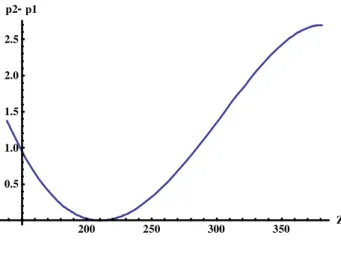
200 250 300 350 Z 0.5 1.0 1.5 2.0 2.5 p2-p1
Figure 9: The solution
We now must find the optimal ZAsol
1 . The corresponding point on the
iso-cost curve must be such that both p1 = p2 and ˙p1 = ˙p2 that is, after time
elimination, such that
psol1 (ZAsol; Z1Asol) = psol2 (ZAsol; Z1Asol) and
p0sol
1 (ZAsol; Z1Asol) = p0sol2 (ZAsol; Z1Asol))
Figure (??) describes the optimal path of p2 − p1, associated with the
optimal value of ZA
1 , in the exemple we use later in our simulations. The
optimal point ZA is the one for which the curve reaches a local minimum
where p2 − p1 = 0. For a larger value of Z1A, the value p2 − p1 is always
positive. For a lower value, p2− p1 takes negative values but there is no point
where both p2− p1 and its derivative are simultaneously zero.
References
References
[1970] Arrow K. J. and M. Kurz, Public investment, the rate of return, and
optimal fiscal policy, Johns Hopkins Press.
[2012] d’Autume A., The behavior of a competitive extraction firm: avoiding the most rapid approach, mimeo.
[2008] Bureau D. , Prix de référence CO2 et calcul économique, mimeo [2008] Chakravorty U., M. Moreaux and M. Tidball (2008), Ordering the
extraction of polluting nonrenewable resources. American Economic
Review 98 (3), June 2008, 1128-44.
[1980] Hanson D.A. Increasing extraction costs and resource prices : some further results, Bell Journal of Economics, 11-1, 335-342
[1976] Heal G., The relationship between price and extraction cost for a resource with a backstop technology, Bell Journal of Economics, 7-2, 371-378
[2011] Hoel M., Carbon taxes and the green paradox, mimeo
[1992] Leonard D. and N. V. Long, Optimal Control Theory and Static
Op-timization in Economics, Cambridge University Press.
[1975] Spence M. and D. Starrett, Most Rapid Approach Paths in Accumu-lation Problems, International Economic Review, 16-2, 388-403. [2011] van der Ploeg F. and C. Withagen 2011, Too little oil, too much coal.
Optimal carbon tax and when to phase in oil, coal and renewables, forthcoming Journal of Public Economics