HAL Id: halshs-00754557
https://hal-pjse.archives-ouvertes.fr/halshs-00754557
Submitted on 29 May 2020
HAL is a multi-disciplinary open access archive for the deposit and dissemination of sci-entific research documents, whether they are pub-lished or not. The documents may come from teaching and research institutions in France or abroad, or from public or private research centers.
L’archive ouverte pluridisciplinaire HAL, est destinée au dépôt et à la diffusion de documents scientifiques de niveau recherche, publiés ou non, émanant des établissements d’enseignement et de recherche français ou étrangers, des laboratoires publics ou privés.
Anthony Atkinson, Thomas Piketty, Emmanuel Saez
To cite this version:
Anthony Atkinson, Thomas Piketty, Emmanuel Saez. Top Incomes in the Long Run of
His-tory. Journal of Economic Literature, American Economic Association, 2011, 49 (1), pp.3-71. �10.1257/jel.49.1.3�. �halshs-00754557�
3 1. Introduction
T
here has been a marked revival of interest in the study of the distribu-tion of top incomes using income tax data. Beginning with the research by Piketty ofthe long run distribution of top incomes in France (Thomas Piketty 2001, 2003), there has been a succession of studies con-structing top income share time series over the long run for more than twenty coun-tries. In using data from the income tax records, these studies use similar sources and methods as the pioneering study for the United States by Simon Kuznets (1953). Kuznets’s estimates were not, how-ever, systematically updated and, in more recent years, household survey data have become the primary source for the empirical analysis
Top Incomes in the
Long Run of History
Anthony B. Atkinson, Thomas Piketty, and Emmanuel Saez
*A recent literature has constructed top income shares time series over the long run for more than twenty countries using income tax statistics. Top incomes represent a small share of the population but a very significant share of total income and total taxes paid. Hence, aggregate economic growth per capita and Gini inequality indexes are sensitive to excluding or including top incomes. We discuss the esti-mation methods and issues that arise when constructing top income share series, including income definition and comparability over time and across countries, tax avoidance, and tax evasion. We provide a summary of the key empirical findings. Most countries experience a dramatic drop in top income shares in the first part of the twentieth century in general due to shocks to top capital incomes during the wars and depression shocks. Top income shares do not recover in the imme-diate postwar decades. However, over the last thirty years, top income shares have increased substantially in English speaking countries and in India and China but not in continental European countries or Japan. This increase is due in part to an unprecedented surge in top wage incomes. As a result, wage income comprises a larger fraction of top incomes than in the past. Finally, we discuss the theoretical and empirical models that have been proposed to account for the facts and the main questions that remain open. (JEL D31, D63, H26, N30)
* Atkinson: Nullfield College, Oxford and London School of Economics. Piketty: Paris School of Economics. Saez: University of California, Berkeley. We are grateful to Facundo Alvaredo, editor Roger Gordon, Stephen Jenkins, and four anonymous referees for helpful comments and discussions.
of inequality.1 The underlying income tax
data continued to be available but remained in the shade for a long period. This relative neglect by economists adds to the interest of the findings of recent tax-based research.
The research surveyed here covers a wide variety of countries and opens the door to the comparative study of top incomes using income tax data. In contrast to existing international databases, generally restricted to the post-1970 or post-1980 period, the top income data cover a much longer period, which is important because struc- tural changes in income and wealth distri-butions often span several decades. In order to properly understand such changes, one needs to be able to put them into broader historical perspective. The new data pro- vide estimates that cover much of the twen-tieth century and in some cases go back to the nineteenth century—a length of time series familiar to economic historians but unusual for most economists. Moreover, the tax data typically allow us to decom-pose income inequality into labor income and capital income components. Economic mechanisms can be very different for the distribution of labor income (demand and supply of skills, labor market institutions, etc.) and the distribution of capital income (capital accumulation, credit constraints, inheritance law and taxation, etc.), so that it is difficult to test these mechanisms using data on total incomes.
This paper surveys the methodology, main findings, and perspectives emerg-ing from this collective research project on the dynamics of income distribution. Starting with Piketty (2001), those stud-ies have been published separately as monographs or journal articles. Recently,
1 The Kuznets series itself remained very influential in the economic history literature on U.S. inequality (see, e.g., Jeffrey G. Williamson and Peter H. Lindert 1980 and Lindert 2000).
those studies have been gathered in two edited volumes (Anthony B. Atkinson and Piketty 2007, 2010), which contain twenty-two country specific chapters along with a general summary chapter (Atkinson, Piketty, and Emmanuel Saez 2010), and a methodological chapter (Atkinson 2007b) upon which this survey draws extensively.2
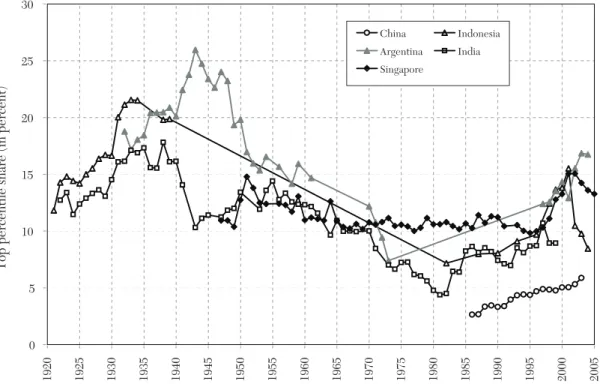
We focus on the data series produced in this project on the grounds that they are fairly homogenous across countries, annual, long-run, and broken down by income source for most countries. They cover twenty-two countries, including many European countries (France, Germany, Netherlands, Switzerland, United Kingdom, Ireland, Norway, Sweden, Finland, Portugal, Spain, Italy), Northern America (United States and Canada), Australia and New Zealand, one Latin American country (Argentina), and five Asian countries (Japan, India, China, Singapore, Indonesia). They cover peri-ods that range from 15 years (China) and 30 years (Italy) to 120 years (Japan) and 132 years (Norway). Hence they offer a unique opportunity to better understand the dynamics of income and wealth distribution and the interplay between inequality and growth. The complete database is available online at the Paris School of Economics at http://g-mond.parisschoolofeconomics.eu/ topincomes/.
To be sure, our series also suffer from important limitations, and we devote con-siderable space to a discussion of these. First, the series measure only top income shares and hence are silent on how inequal-ity evolves elsewhere in the distribution. Second, the series are largely concerned with gross incomes before tax. Thirdly, the defini-tion of income and the unit of observagross incomes before tax. Thirdly, the defini-tion
2 The reader is also referred to the valuable survey by Andrew Leigh (2009). Shorter summaries have also been presented in Piketty (2005, 2007), Piketty and Saez (2006), and Saez (2006).
(the individual versus the family) vary across countries making comparability of levels across countries more difficult. Even within a country, there are breaks in comparability that arise because of changes in tax legislation affecting the definition of income, although most studies try to correct for such changes to create homogenous series. Finally and perhaps most important, our series might be biased because of tax avoidance and tax evasion. Many of the studies spend consider- able time exploring in detail how tax legisla-tion changes can affect the series. The series created can therefore also be used to tackle the classical public economics issue of the response of reported income to changes in tax law.
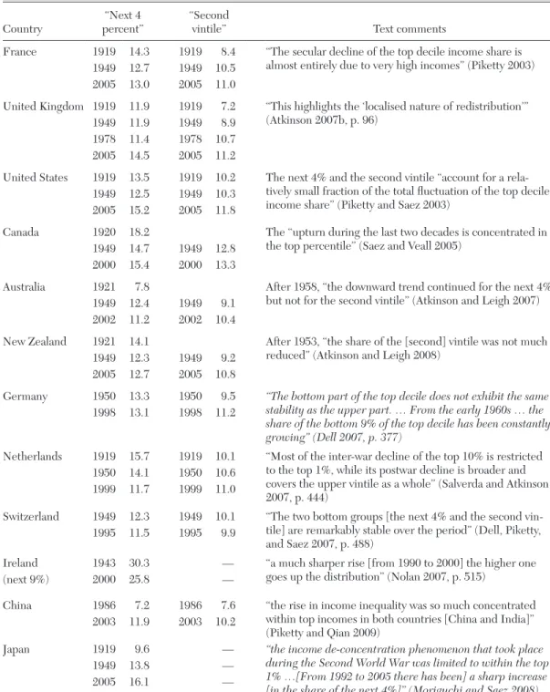
We obtain three main empirical results. First, most countries experienced a sharp drop in top income shares in the first half of the twentieth century. In these coun-tries, the fall in top income shares is often concentrated around key episodes such as the World Wars or the Great Depression. In some countries however, especially those that stayed outside World War II, the fall is more gradual during the period. In all coun-tries for which income composition data are available, in the first part of the century, top percentile incomes were overwhelmingly composed of capital income (as opposed to labor income). Therefore, the fall in the top percentile share is primarily a capital income phenomenon: top income shares fall because of a reduction in top wealth concentration. In contrast, upper income groups below the top percentile such as the next 4 percent or the second vingtile, which are comprised pri-marily of labor income, fall much less than the top percentile during the first half the twentieth century.
By 1949, the dispersion in top percen-tile income shares across the countries studied had become small. In the second half of the twentieth century, top percen-tile shares experienced a U-shape pattern,
with further declines during the immedi-ate postwar decades followed by increases in recent decades. However, the degree of the U-shape varies dramatically across coun-tries. In all of the Western English speaking countries (in Europe, North America, and Australia and New Zealand), and in China and India, there was a substantial increase in top income shares in recent decades, with the United States leading the way both in terms of timing and magnitude of the increase. Southern European countries and Nordic countries in Europe also experience an increase in top percentile shares although less in magnitude than in English speaking countries. In contrast, Continental European countries (France, Germany, Netherlands, Switzerland) and Japan experience a very flat
U-shape with either no or modest increases
in top income shares in recent decades. Third, as was the case for the decline in the first half of the century, the increase in top income shares in recent decades has been quite concentrated with most of the gains accruing to the top percentile with much more modest gains (or even none at all) for the next 4 percent or the second vingtile. However, in most countries, a sig-nificant portion of the gains are due to an increase in top labor incomes, and especially wages and salaries. As a result, the fraction of labor income in the top percentile is much higher today in most countries than earlier in the twentieth century. The rest of this paper is organized as fol-lows. In section 2, we provide motivation for the study of top incomes. In section 3, we present the methodology used to construct the database using tax statistics, and dis-cuss in details the key issues and limitations. Section 4 presents a summary of the main descriptive findings. Section 5 discusses the theoretical and empirical models that have been proposed to account for the facts while section 6 discusses how those models and explanations fit with the empirical findings.
2. Motivation
The share of total income going to top income groups has risen dramatically in recent decades in the United States and in many other (but not all) countries. Taking the U.S. case, we see from figure 1 the changes since 1917 in the top decile (pre-tax) income share (from Piketty and Saez 2003 series including capital gains updated to 2007). After a precipitous (10 percent-age point) decline during World War II and stability in the postwar decades, the top decile share has surged (a rise of more than 10 percentage points) since the 1970s and reached almost 50 percent by 2007,
the highest level on record. Figure 2 breaks down the top decile into the top percentile, the next 4 percent (top 5 percent excluding the top 1 percent), and the second vingtile (top 10 percent excluding the top 5 percent). It shows that most of the changes in the top decile are due to dramatic changes in the top percentile, which rose from 8.9 percent in 1976 to 23.5 percent in 2007. As shown on figure 3, the share of an even wealthier group—the top 0.1 percent—has more than quadrupled from 2.6 percent to 12.3 percent over this period. Figure 3 also displays the composition of top 0.1 percent incomes and shows that, although the levels of the top 0.1 percent income share is as high today as Figure 1. The Top Decile Income Share in the United States, 1917–2007. Notes: Income is defined as market income including realized capital gains (excludes government transfers). In 2007, top decile includes all families with annual income above $109,600. Source: Piketty and Saez (2003), series updated to 2007. 25% 30% 35% 40% 45% 50% 1917 1922 1927 1932 1937 1942 1947 1952 1957 1962 1967 1972 1977 1982 1987 1992 1997 2002 2007
in the pre–Great Depression era, wages and salaries now form a much greater fraction of top incomes than in the past.
Why do these increases at the top mat-ter? Several answers can be given. The most general is that people have a sense of fairness and care about the distribution of economic resources across individuals in society. As a result, all advanced economies have set in place redistributive policies such as taxation— and in particular progressive taxation, and transfer programs, which effectively redis-tribute a significant share of National Product across income groups. Importantly, different
parts of the distribution are interdependent. Here we consider three more specific eco-nomic reasons why we should be interested in the top income groups: their impact on overall growth and resources, their impact on overall inequality, and their global significance. 2.1 Impact on Overall Growth and
Resources
The textbook definition of income by econ-omists refers to “command over resources.” Are however the rich sufficiently numerous and sufficiently in receipt of income that they make an appreciable difference to the 0% 5% 10% 15% 20% 25% 1913 1918 1923 1928 1933 1938 1943 1948 1953 1958 1963 1968 1973 1978 1983 1988 1993 1998 2003
Share of total income accruing to each group
Top 1% (incomes above $398,900 in 2007) Top 5–1% (incomes between $155,400 and $398,900) Top 10–5% (incomes between $109,600 and $155,400)
Figure 2. Decomposing the Top Decile US Income Share into three Groups, 1913–2007 Notes: Income is defined as market income including capital gains (excludes all government transfers). Top 1 percent denotes the top percentile (families with annual income above $398,900 in 2007). Top 5–1 percent denotes the next 4 percent (families with annual income between $155,400 and $398,900 in 2007). Top 10–5 percent denotes the next 5 percent (bottom half of the top decile, families with annual income between $109,600 and $155,400 in 2007). Source: Piketty and Saez (2003), series updated to 2007.
overall control of resources? First, although the top 1 percent is by definition only a small share of the population, it does capture more than a fifth of total income—23.5 percent in the United States as of 2007. Second and even more important, the surge in top incomes over the last thirty years has a dra-matic impact on measured economic growth. As shown in table 1, U.S. real income per family grew at a modest 1.2 percent annual rate from 1976 to 2007. However, when excluding the top 1 percent, the average real income of the bottom 99 percent grew at an annual rate of only 0.6 percent, which implies that the top 1 percent captured 58 percent
of real economic growth per family during that period (column 4 in table 1). The effects of the top 1 percent on growth can be seen even more dramatically in two contrast-ing recent periods of economic expansion, 1993–2000 (Clinton administration expan-sion) and 2002–07 (Bush administration expansion). Table 1 shows that, during both expansions, the real incomes of the top 1 per-cent grew extremely quickly at an annual rate over 10.1 and 10.3 percent respectively. However, while the bottom 99 percent of incomes grew at a solid pace of 2.7 percent per year from 1993 to 2000, these incomes grew only 1.3 percent per year from 2002
0% 2% 4% 6% 8% 10% 12% 1916 1921 1926 1931 1936 1941 1946 1951 1956 1961 1966 1971 1976 1981 1986 1991 1996 2001 2006 Capital Gains Capital Income Business Income Salaries Figure 3. The Top 0.1 Percent Income Share and Composition, 1916–2007 Notes: The figure displays the top 0.1 percent income share and its composition. Income is defined as market income including capital gains (excludes all government transfers). Salaries include wages and salaries, bonus, exercised stock-options, and pensions. Business income includes profits from sole proprietorships, partnerships, and S-corporations. Capital income includes interest income, dividends, rents, royalties, and fiduciary income. Capital gains includes realized capital gains net of losses. Source: Piketty and Saez (2003), series updated to 2007.
to 2007. Therefore, in the economic expan-sion of 2002–07, the top 1 percent captured over two-thirds (65 percent) of income growth. Those results may help explain the gap between the economic experiences of the public and the solid macroeconomic growth posted by the U.S. economy from 2002 to the peak of 2007. Those results may also help explain why the dramatic growth in top incomes during the Clinton adminis-tration did not generate much public outcry while there has been an extraordinary level of attention to top incomes in the U.S. press and in the public debate in recent years. Such changes also matter in international comparisons. For example, average real incomes per family in the United States grew by 32.2 percent from 1975 to 2006 while they grew only by 27.1 percent in France during the same period (Piketty 2001 and Camille Landais 2007), showing that the macro-economic performance in the United States was better than the French one during this
period. Excluding the top percentile, aver-age U.S. real incomes grew only 17.9 percent during the period while average French real incomes—excluding the top percentile—still grew at much the same rate (26.4 percent) as for the whole French population. Therefore, the better macroeconomic performance of the United States versus France is reversed when excluding the top 1 percent.3
More concretely, we can ask whether increased taxes on the top income group would yield appreciable revenue that could be deployed to fund public goods or redistri- bution? This question is of particular inter-est in the current U.S. policy debate where large government deficits will require raising tax revenue in coming years. The standard
3 It is important to note that such international growth
comparisons are sensitive to the exact choice of years compared, the price deflator used, the exact defini-tion of income in each country, and hence are primarily illustrative. TABLE 1 Top Percentile Share and Average Income Growth in the United States Average income real annual growth Top 1% incomes real annual growth Bottom 99% incomes real annual growth Fraction of total growth captured by top 1% (1) (2) (3) (4) Period 1976–2007 1.2% 4.4% 0.6% 58% Clinton expansion 1993–2000 4.0% 10.3% 2.7% 45% Bush expansion 2002–2007 3.0% 10.1% 1.3% 65% Notes: Computations based on family market income including realized capital gains (before individual taxes). Incomes are deflated using the Consumer Price Index (and using the CPI-U-RS before 1992). Column (4) reports the fraction of total real family income growth captured by the top 1 percent. For example, from 2002 to 2007, average real family incomes grew by 3.0 percent annually but 65 percent of that growth accrued to the top 1 percent while only 35 percent of that growth accrued to the bottom 99 percent of U.S. families. Source: Piketty and Saez (2003), series updated to 2007 in August 2009 using final IRS tax statistics.
response by many economists in the past has been that “the game is not worth the candle.” Indeed, net of all federal taxes, in the United States in 1976 the top percentile received only 5.8 percent of total pretax income, an amount equal to 24 percent of all federal taxes (individual, corporate, estate taxes, and social security and health contributions) in that year. However, by 2007, net of all federal taxes, the top percentile received 17.3 percent of total pretax income, or about 74 percent of all federal taxes raised in 2007.4 Therefore, it is clear that the surge in the top percentile share has greatly increased the “tax capacity” at the top of the income distribution. In budgetary terms, this cannot be ignored.5
2.2 Impact on Overall Inequality
It might be thought that top shares have little impact on overall inequality. If we draw a Lorenz curve, defined as the share of total income accruing to those below percentile p, as p goes from 0 (bottom of the distribution) to 100 (top of the distribution), then the top 1 percent would scarcely be distinguishable on the horizontal axis from the vertical endpoint, and the top 0.1 percent even less so. The most commonly used summary measure of overall inequality, the Gini coefficient, is more sensi- tive to transfers at the center of the distribu-tion than at the tails. (The Gini coefficient is defined as the ratio of the area between the Lorenz curve and the line of equality over the total area under the line of equality.) 4 The 5.8 percent and 17.3 percent figures are based on
average tax rates by income groups presented in Piketty and Saez (2006). We exclude the corporate tax and the employer portion of payroll taxes as the pretax income share series are based on market income after corpo-rate taxes and employer payroll taxes. We have 5.8 per-cent = 8.8 percent * (1 − 0.262 − 0.016/2 − .068) and 17.3 percent = 23.5 percent * (1 − .225 − 0.03/2 − 0.022). The percentage of all federal taxes is obtained using total federal average tax rates that are 24.7 percent and 23.7 per-cent in 1976 and 2007 from Piketty and Saez (2006).
5 We discuss the important issue of the behavioral responses of top incomes to taxes in section 5.
But top shares can materially affect overall inequality, as may be seen from the follow-ing calculation. If we treat the very top group as infinitesimal in numbers, but with a finite share S* of total income, then, graphically, the Lorenz curve reaches 1 − S* just below
p = 100. As a result, the total Gini
coeffi-cient can be approximated by S* + (1 − S*)
G, where G is the Gini coefficient for the
population excluding the top group (Atkinson 2007b). This means that, if the Gini coefficient for the rest of the population is 40 percent, then a rise of 14 percentage points in the top share, as happened with the share of the top 1 percent in the United States from 1976 to 2006, causes a rise of 8.4 percentage points in the overall Gini. This is larger than the official Gini increase from 39.8 percent to 47.0 per-cent over the 1976–2006 period based on U.S. household income in the Current Population Survey (U.S. Census Bureau 2008, table A3).6
2.3 Top Incomes in a Global Perspective The analysis so far has considered the role of top incomes in a purely national context, but it is evident that the rich, or at least the super-rich, are global players. What however is their quantitative significance on a world scale? Does it matter if the share of the top 1 percent in the United States doubles? The top 1 percent in the United States constitutes 1.5 million tax units. How do they fit into a world of some 6 billion people? According to the estimates of Francois Bourguignon and Christian Morrisson (2002), the world Gini coefficient went from 61 percent in 1910 to 64 percent in 1950 and then to 65.7 percent in 1992, as displayed in figure 4 (full triangle series, right y-axis).7 How did the evolution of top income shares in richer countries, which 6 The relation between top shares and overall inequality is explored further by Leigh (2007). 7 As spelled out in Bourguignon and Morrisson (2002),
strong assumptions are required to obtain a worldwide Gini coefficient based on country level inequality statistics.
fell during the first part of the twentieth cen-tury and increased sharply in some countries in recent decades, affect this picture?
To address this question, Atkinson (2007b) defines the “globally rich” as those with more than twenty times the mean world income, which in 1992 meant above $100,000. Atkinson uses the distribution of income among world citizens constructed by Bourguignon and Morrisson (2002) combined with a Pareto imputation for the top of the distribution8 to estimate the number of 8 The Pareto parameter is estimated using the ratio of
the top 5 percent income share to the top decile income share (see equation (4) below), both being reported in
“globally rich.” In 1992, there were an esti-mated 7.4 million people with incomes above this level, more than a third of them in the United States. They constituted 0.14 per-cent of the world population but received 5.4 percent of total world income. As shown on figure 4 (left y-axis), as a proportion of the world population, the globally rich fell from 0.23 percent in 1910 to 0.1 percent in 1970, mirroring the decline in top income shares recorded in individual countries. Therefore,
Bourguignon and Morrisson (2002). Because those top income shares are often based on survey data (and not tax data), they likely underestimate the magnitude of the changes at the very top. 0.00% 0.05% 0.10% 0.15% 0.20% 0.25% 1910 1915 1920 1925 1930 1935 1940 1945 1950 1955 1960 1965 1970 1975 1980 1985 1990
% of world with income above 20 times world mean
45% 50% 55% 60% 65% 70%
Worldwide Gini coefficient
Fraction super rich Fraction super rich (from US) World Gini
Figure 4. The Globally Super Rich and Worldwide Gini, 1910–1992
Sources: Fraction super rich series is defined as the fraction of citizens in the world with income above
twenty times the world mean. Estimated by Atkinson (2007) using Bourguignon and Morrisson (2002) series.
Fraction super rich (from U.S.) series is defined as the number of U.S. citizens with income above twenty times the world mean divided by the world citizens. Estimated by Atkinson (2007) using Bourguignon and Morrisson (2002) series. Worldwide Gini series is the Gini coefficient among world citizens estimated by Bourguigon and Morrisson (2002).
although overall inequality among world citi-zens increased, there was a compression at the top of the world distribution. But from 1970, we see a reversal and a rise in the pro-portion of globally rich above the 1950 level. The number of globally rich doubled in the United States between 1970 and 1992, which accounts for half of the worldwide increase in the number of “globally rich” and hence makes a perceptible difference to the world distribution.
2.4 Summary
There are a number of reasons for study-ing the development of top income shares. Understanding the extent of inequality at the top and the relative importance of differ-ent factors leading to increasing top shares is important in the design of public policy. Concern about the rise in top shares in a num-ber of countries has led to proposals for higher top income tax rates; other countries are con-sidering limits on remuneration and bonuses. The global distribution is coming under increasing scrutiny as globalization proceeds.
3. Methodology and Limitations 3.1 Methodology
The value of the tax data lies in the fact that, early on, the tax authorities in most countries began to compile and publish tabu-lations based on the exhaustive set of income tax returns.9 These tabulations generally
report for a large number of income brackets
9 The first income tax distribution published for the United Kingdom related to 1801 (see Josiah C. Stamp 1916) but no further figures on total income are avail-able for the nineteenth century on account of the move to a schedular system. The publication of regular U.K. distributional data only commenced with the introduc-tion of supertax in 1909. Distributional data were however already by then being produced in certain parts of the British Empire. For example, in 1905, the State of Victoria (Australia) supplied a table of the distribution of income
the corresponding number of taxpayers, as well as their total income and tax liability. They are usually broken down by income source: capital income, wage income, busi-ness income, etc. Table 2 shows an example of such a table from the British super-tax data for fiscal year 1911–12. These data were used by Arthur L. Bowley (1914), but it was not until the pioneering contribution of Kuznets (1953) that researchers began to combine the tax data with external estimates of the total population and the total income to estimate top income shares.10
The data in table 2 illustrate the three methodological problems addressed in this section when estimating top income shares. The first is the need to relate the number or persons to a control total to define how many tax filers represent a given fractile such as the top percentile. In the case of the United Kingdom in 1911–12, only a very small fraction of the population is subject to the super-tax: less than 12,000 taxpayers out of a total population of over twenty million tax units, i.e., not much more than 0.05 per- cent. The second issue concerns the defini-tion of income and the relation to an income control total used as the denominator in the top income share estimation. The third prob-lem is that, for much of the period, the only data available are tabulated by ranges so that interpolation estimation is required. Micro data only exist in recent decades. Note also that the tabulated data vary considerably in the number of ranges and the information provided for each range. Different meth-ods have been used for interpolation, such
in 1903 in response to a request for information from the U.K. government (House of Commons 1905, p. 233).
10 Before Kuznets, U.S. tax statistics had been used pri-marily to estimate Pareto parameters as this does not require estimating total population and total income controls (see below): see for example William L. Crum (1935), Norris O. Johnson (1935 and 1937), and Rufus S. Tucker (1938). The drawback is that Pareto parameters only capture dispersion of incomes in the top tail and—unlike top income shares— do not relate top incomes to average incomes.
as the Pareto interpolation discussed in the next subsection and the split histogram (see Atkinson 2005). 3.1.1 Pareto Interpolation The basic data are in the form of grouped tabulations, as in table 2, where the intervals do not in general coincide with the percent-age groups of the population with which we are concerned (such as the top 1 percent). We have therefore to interpolate in order to arrive at values for summary statistics such as the shares of total income. Moreover, some authors have extrapolated upwards into the open upper interval and downwards below the lowest range tabulated. The Pareto law for top incomes is given by the following (cumu-lative) distribution function F(y) for income y: (1) 1 − F(y) = (k/y)α (k > 0, α > 1), where k and α are given parameters, α is called the Pareto parameter. The
corresponding density function is given by f (y) = αkα/y(1+α). The key property of Pareto distributions is that the ratio of average income y*(y) of individuals with income above y to y does not depend on the income threshold y:
(2) y*(y) =
[
∫
z >y z f (z) dz]
/[
∫
z>y f (z) dz]
=
[
∫
z>y d z/zα]
/[
∫
z>y d z/z(1+α)]
= α y/(α − 1),i.e., y*(y)/y = β , with β = α/(α − 1). That is, if β = 2, the average income of individuals with income above $100,000 is $200,000 and the average income of individu-als with income above $1 million is $2 million. Intuitively, a higher β means a fatter upper tail of the distribution. From now on, we refer to β as the inverted Pareto coefficient. Throughout this paper, we choose to focus
TABLE 2
Example of Income Tax Data: UK Super-Tax, 1911–12
Income class Number of persons Total income assessed At least but less than £5,000 £10,000 7,767 £52,810,069 £10,000 £15,000 2,055 £24,765,153 £15,000 £20,000 798 £13,742,318 £20,000 £25,000 437 £9,653,890 £25,000 £35,000 387 £11,385,691 £35,000 £45,000 188 £7,464,861 £45,000 £55,000 106 £5,274,658 £55,000 £65,000 56 £3,295,110 £65,000 £75,000 37 £2,590,606 £75,000 £100,000 56 £4,929,787 £100,000 — 66 £12,183,724 Total 11,953 £148,095,867 Source: Annual Report of the Inland Revenue for the Year 1913–14: table 140, p. 155.
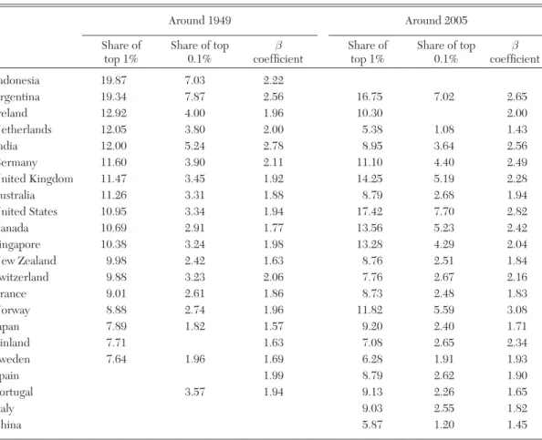
on the inverted Pareto coefficient β (which has more intuitive economic appeal) rather than the standard Pareto coefficient α. Note that there exists a one-to-one, monotonically decreasing relationship between the α and β coefficients, i.e., β = α/(α − 1) and α = β/ (β − 1) (see table 3).11
Vilfredo Pareto (1896, 1896–1897), in the 1890s using tax tabulations from Swiss cantons, found that this law approximates remarkably well the top tails of the income or wealth distributions. Since Pareto, raw
11 Put differently, (β − 1) is the inverse of (α − 1).
It should be noted that this is different from the inverse-Pareto coefficient used by Lee C. Soltow (1969), although this too increases as the tail becomes fatter.
tabulations by brackets produced by tax administrations have often been used to esti-mate Pareto parameters.12 A number of the
top income studies conclude that the Pareto approximation works remarkably well today, in the sense that for a given country and a given year, the β coefficient is fairly invariant with y. However a key difference with the early Pareto literature, which was implicitly looking for some universal stability of income and wealth distributions, is that our much
12 There also exists a voluminous theoretical literature trying to explain why Pareto laws fit the top tails of income and wealth distributions. We survey some of these theoret-ical models in section 5 below. Pareto laws have also been applied in several areas outside income and wealth distri-bution (see, e.g., Xavier Gabaix 2009 for a recent survey). TABLE 3 Pareto-Lorenz α Coefficients versus Inverted-Pareto-Lorenz β Coefficients α β = α/(α − 1) β α = β/(β − 1) 1.10 11.00 1.50 3.00 1.30 4.33 1.60 2.67 1.50 3.00 1.70 2.43 1.70 2.43 1.80 2.25 1.90 2.11 1.90 2.11 2.00 2.00 2.00 2.00 2.10 1.91 2.10 1.91 2.30 1.77 2.20 1.83 2.50 1.67 2.30 1.77 3.00 1.50 2.40 1.71 4.00 1.33 2.50 1.67 5.00 1.25 3.00 1.50 10.00 1.11 3.50 1.40 Notes: (1) The “α” coefficient is the standard Pareto-Lorenz coefficient commonly used in power-law distribution formu-las: 1−F(y) = (A/y)α and f(y) = αAα/y1+α (A>0, α>1, f(y) = density function, F(y) = distribution function, 1−F(y) = proportion of population with income above y). A higher coefficient α means a faster convergence of the density toward zero, i.e., a less fat upper tail. (2) The “β” coefficient is defined as the ratio y*(y)/y, i.e., the ratio between the average income y*(y) of individuals with income above threshold y and the threshold y. The characteristic property of power laws is that this ratio is a constant, i.e., does not depend on the threshold y. Simple computations show that β = y*(y)/y = α/(α−1), and conversely α = β/(β−1).
larger time span and geographical scope allows us to document the fact that Pareto coefficients vary substantially over time and across countries.
From this viewpoint, one additional advantage of using the β coefficient is that a higher β coefficient generally means larger top income shares and higher income inequality (while the reverse is true with the more commonly used α coefficient). For instance, in the United States, the β coefficient (estimated at the top percen-tile threshold and excluding capital gains) increased gradually from 1.69 in 1976 to 2.89 in 2007 as top percentile income share surged from 7.9 percent to 18.9 percent.13
In a country like France, where the β coef-ficient has been stable around 1.65–1.75 since the 1970s, the top percentile income share has also been stable around 7.5 per-cent–8.5 percent, except at the very end of the period.14 In practice, we shall see that β
coefficients typically vary between 1.5 and 3: values around 1.5–1.8 indicate low inequal-ity by historical standards (with top 1 percent income shares typically between 5 percent and 10 percent), while values around or above 2.5 indicate very high inequality (with top 1 percent income shares typically around 15 percent–20 percent or higher). In the case of the United Kingdom in 1911–12, a high inequality country, one can easily com-pute from table 2 that the average income of taxpayers above £5,000 was £12,390, i.e., the β coefficient was equal to 2.48.15 In practice, it is possible to verify whether Pareto (or split histogram) interpolations are 13 When we include capital gains, the rise of the β coef-ficient is even more dramatic, from 1.82 in 1976 to 3.42 in 2007. 14 See Atkinson and Piketty (2007, 2010). 15 The stability of β coefficients (for a given country and a given year) only holds for top incomes, typically within the top percentile. For incomes below the top percentile, the β coefficient takes much higher values (for very small incomes it goes to infinity). Within the top percentile, the β
accurate when large micro tax return data with over-sampling at the top are available as is the case in the United States since 1960. Those direct comparisons show that errors due to interpolations are typically very small if the number of brackets is sufficiently large and if income amounts are also reported. In the end, the error due to Pareto interpola- tion is likely to be dwarfed by various adjust-ments and imputations required for making series homogeneous, or errors in the estima-tion of the income control total (see below). 3.1.2 Control Total for Population
In some countries, such as Canada, New Zealand from 1963, or the United Kingdom from 1990, the tax unit is the individual. In that case, the natural control total is the adult population defined as all residents at or above a certain age cutoff, and the top percentile share will measure the share of total income accruing to the top percentile of adult individuals. In other countries, tax units are families. In the United Kingdom, for example, the tax unit until 1990 was defined as a married couple living together, with dependent children (without inde-pendent income), or as a single adult, with dependent children, or as a child with inde-pendent income. The control total used by Atkinson (2005) for the U.K. population for this period is the total number of people aged 15 and over minus the number of mar-ried females. In the United States, married women can file tax separate returns, but the number is “fairly small (about 1 percent of all returns in 1998)” (Piketty and Saez 2003). Piketty and Saez therefore treat the data as coefficient varies slightly, and falls for the very top incomes (at the level of the single richest taxpayer, β is by definition equal to 1), but generally not before the top 0.1 percent or top 0.01 percent threshold. In the example of table 2, one can easily compute that the β coefficient gradually falls from 2.48 at the £5,000 threshold to 2.28 at the £10,000 threshold and 1.85 at the £100,000 threshold (with only sixty-six taxpayers left).
relating to families and take as a control total the sum of married males and all nonmarried individuals aged 20 and over.
What difference does it make to use the individual unit versus the family unit? If we treat all units as weighted equally (so couples do not count twice) and take total income, then the impact of moving from a couple-based to an individual-based system depends on the joint distribution of income. A useful special case is where the marginal distribu-tions are such that the upper tail is Pareto in form. Suppose first that all rich people are either unmarried or have partners with zero income. The number of individuals with incomes in excess of $Y is the same as the number of families and their total income is the same. The overall income control total is unchanged but the total number of individu-als exceeds the total number of tax units (by a factor written as (1 + m)). This means that to locate the top p percent, we now need to go further down the distribution, and, given the Pareto assumption, the share rises by a factor (1 + m)1-1/α. With α = 2 and m = 0.4, this equals 1.18. On the other hand, if all rich tax units consist of couples with equal incomes, then the same amount (and share) of total income is received by 2/(1 + m) times the fraction of the population. In the case of the Pareto distribution, this means that the share of the top 1 percent is reduced by a factor (2/(1 + m))1−1/α. With α = 2 and
m = 0.4, this equals 1.2. We have therefore
likely bounds on the effect of moving to an individual basis. If the share of the top 1 per-cent is 10 percent, then this could be increased to 11.8 percent or reduced to 8.3 percent. The location of the actual figure between these bounds depends on the joint distribution, and this may well have changed over the century.
Saez and Michael R. Veall (2005), in the case of Canada, can compute top wage income shares both on an individual and family base since 1982. They find that indi-vidual based top shares are slightly higher
(by about 5 percent). Most importantly, the family based and individual based top shares track each other extremely closely. Similarly, Wojciech Kopczuk, Saez, and Jae Song (2010) compute individual based top wage income shares and show that they track also very closely the family based wage income shares estimated by Piketty and Saez (2003). This shows that changes in the correlation of earnings across spouses have played a neg-ligible role in the surge in top wage income shares in North America. However, shifting from family to individual units does have an impact on the level of top income shares and creates a discontinuity in the series.16
3.1.3 Control Total for Income
The aim is to relate the amounts recorded in the tax data (numerator of the top share) to a comparable control total for the full popu-lation (denominator of the top share). This is a matter that requires attention, since differ-ent methods are employed, which may affect comparability overtime and across countries. One approach starts from the income tax data and adds the income of those not covered (the “nonfilers”). This approach is used for example for the United Kingdom (Atkinson 2005), and the United States (Piketty and Saez 2003) for the years since 1944. The approach in effect takes the definition of income embodied in the tax legislation, and the resulting estimates will change with variations in the tax law. For example, short-term capital gains have been included to varying degrees in taxable income in the United Kingdom. A second approach, 16 Most studies correct for such discontinuities by cor- recting series to eliminate the discontinuity. Absent over-lapping data at both the family and individual levels, such a correction has to be based on strong assumptions (for example that the rate of growth in income shares around the discontinuity is equal to the average rate of growth the year before and the year after the discontinuity). We flag studies in table 4 where no correction for such discontinui-ties are made.
pioneered by Kuznets (1953), starts from an external control total, typically derived from the national accounts. This approach is fol-lowed for example in France (Piketty 2001, 2003), or the United States for the years prior to 1944. The approach seeks to adjust the tax data to the same basis, correcting for exam-ple for missing income and for differences in timing. In this case, the income of nonfil-ers appears as a residual. This approach has a firmer conceptual base, but there are sig-nificant differences between income concepts used in national accounts and those used for income tax purposes.
The first approach estimates the total income that would have been reported if everybody had been required to file a tax return. Requirements to file a tax return vary across time and across countries. Typically most countries have moved from a situation at the beginning of the last century when a minority filed returns to a situation today where the great majority are covered. For example, in the United States, “before 1944, because of large exemption levels, only a small fraction of individuals had to file tax returns” (Piketty and Saez 2003, p. 4). It should be noted that taxpayers might not need to make a tax return to appear in the statistics. Where there is tax collection at source, as with Pay-As-You-Earn (PAYE) in the United Kingdom, many people do not file a tax return but are covered by the pay records of their employers. Estimates of the income of nonfilers may be related to the average income of filers. For the United States, Piketty and Saez (2003), for the period since 1944, impute to nonfilers a fixed fraction equal to 20 percent of filers’ aver-age income. In some cases, estimates of the income of nonfilers already exist. Atkinson (2005) makes use of the work of the Central Statistical Office for the United Kingdom.
The second approach starts from the national accounts totals for personal income. In the case of the United States, Piketty and
Saez use, for the period 1913–43, a control total equal to 80 percent of (total personal income less transfers). In Canada, Saez and Veall (2005) use this approach for the entire period 1920–2000. How do these national income based calculations relate to the totals in the tax data? In answering this question, it may be helpful to bear in mind the different stages set out schematically below:
Personal sector total income (PI)
minus Nonhousehold income (Nonprofit
institutions such as charities)
equals Household sector total income minus Items not included in tax base
(e.g., employers’ social security contributions and—in some coun-tries—employees’ social security contributions, imputed rent on owner-occupied houses, and nontax-able transfer payments)
equals Household gross income returnable
to tax authorities
minus Taxable income not declared by
filers
minus Taxable income of those not
included in tax returns (“nonfilers”)
equals Declared taxable income of filers.
The use of national accounts totals may be seen as moving down from the top rather than moving up from the bottom by adding the estimated income of nonfilers. The per-centage formulae can be seen as correcting for the nonhousehold elements and for the difference between returnable income and the national accounts definition. Some of the items, such as social security contributions, can be substantial. Piketty and Saez base their choice of percentage for the United States on the experience for the period 1944–98, when they applied estimates of the income of nonfilers.
Given the increasing significance of some of the items (such as employers’ contribu-tions) and of the nonhousehold institutions
(such as pension funds), it is not evident that a constant percentage is appropriate. Since transfers were also smaller at the start of the twentieth century, total household return-able income was then closer to total personal income. Atkinson (2007) compares the two methods in the case of the United Kingdom. He shows that the total income estimated from the first method by estimating the income of nonfilers trends slightly down-wards relative to personal income minus transfers from around 90 percent in the first part of the twentieth century to around 85 percent in the last part of the century. Furthermore, there are substantial short-term variations especially during world war episodes when the national accounts figures appear to be relatively higher by as much as 15–20 percent. Some countries do not have developed national accounts, especially in the earlier periods covered by tax statistics. In that case, the total income control is cho-sen as a fixed percentage of GDP where the percentage is calibrated using later periods when National accounts are more developed. Need for a control total for income is of course avoided if we examine the “shares within shares” that depend solely on popula-tion totals and the income distribution within the top, measured by the Pareto coefficient. This gives a measure of the degree of inequal-ity among the top incomes that may be more robust but does not compare top incomes to the average as top income shares do.
3.1.4 Adjustments for Income Definition In a number of cases, the definition of income used to present the tabulations changes over time. To obtain homogeneous series, such changes need to be corrected for. The most common change in the presen-tation of tabulations is due to shifts from net income (income after deductions) to gross income (income before deductions). When composition information on the amount of deductions by income brackets is available,
the series estimated can be corrected for such changes. If we assume that ranking of individuals by net income and gross income are approximately the same, the correction can be made by simply adding back average deductions bracket by bracket to go from net incomes to gross incomes. This assumption can be checked when micro-data is available as is the case in the United States since 1960 for example (Piketty and Saez 2003). It is also of interest to estimate both series including capital gains and series exclud-ing capital gains (see below). This can also be done if data on amounts of capital gains are available by income brackets. Because capital gains can be quite important at the top (see figure 3), ranking of individuals might change significantly when including or excluding capital gains. The ideal is therefore to have access to micro-data to create tabu-lations both including and excluding capital gains. The micro-data can also be used to assess how ranking changes when excluding capital gains and hence develop simple rules of thumb to construct series excluding capi-tal gains when starting with series including capital gains (or vice versa). This is done in Piketty and Saez (2003) for the period before 1960, the first year when micro-data become available in the United States. 3.1.5 Other Studies
As mentioned above, Kuznets (1953) developed the methodology of combining national accounts with tax statistics to esti-mate top income shares. Before Kuznets, studies using tax statistics were limited to the estimation of Pareto parameters (starting with Pareto 1896 and followed by numerous studies across many countries and time peri-ods) or to situations where the coverage of tax statistics was substantial or could be sup-plemented with additional income data (as in Scandinavian countries, the Netherlands, the German states, or the United Kingdom as we mentioned above). Therefore, there