Normal mode Rossby waves and their effects on chemical composition in the late summer stratosphere

(1)

HAL Id: hal-00303052

https://hal.archives-ouvertes.fr/hal-00303052

Submitted on 14 Aug 2007

HAL is a multi-disciplinary open access

archive for the deposit and dissemination of sci-entific research documents, whether they are pub-lished or not. The documents may come from teaching and research institutions in France or abroad, or from public or private research centers.

L’archive ouverte pluridisciplinaire HAL, est destinée au dépôt et à la diffusion de documents scientifiques de niveau recherche, publiés ou non, émanant des établissements d’enseignement et de recherche français ou étrangers, des laboratoires publics ou privés.

Normal mode Rossby waves and their effects on

chemical composition in the late summer stratosphere

D. Pendlebury, T. G. Shepherd, M. Pritchard, C. Mclandress

To cite this version:

D. Pendlebury, T. G. Shepherd, M. Pritchard, C. Mclandress. Normal mode Rossby waves and their effects on chemical composition in the late summer stratosphere. Atmospheric Chemistry and Physics Discussions, European Geosciences Union, 2007, 7 (4), pp.12011-12033. �hal-00303052�

(2)

ACPD

7, 12011–12033, 2007

Normal mode Rossby waves in the late summer stratosphere D. Pendlebury et al. Title Page Abstract Introduction Conclusions References Tables Figures ◭ ◮ ◭ ◮ Back Close

Full Screen / Esc

Printer-friendly Version Interactive Discussion

EGU

Atmos. Chem. Phys. Discuss., 7, 12011–12033, 2007 www.atmos-chem-phys-discuss.net/7/12011/2007/ © Author(s) 2007. This work is licensed

under a Creative Commons License.

Atmospheric Chemistry and Physics Discussions

Normal mode Rossby waves and their

effects on chemical composition in the

late summer stratosphere

D. Pendlebury1, T. G. Shepherd1, M. Pritchard2, and C. McLandress1

1

University of Toronto, Toronto, Canada

2

University of California, San Diego, USA

Received: 5 July 2007 – Accepted: 27 July 2007 – Published: 14 August 2007 Correspondence to: D. Pendlebury (diane@atmosp.physics.utoronto.ca)

(3)

ACPD

7, 12011–12033, 2007

Full Screen / Esc

Abstract

During past MANTRA campaigns, ground-based measurements of several long-lived chemical species have revealed quasi-periodic fluctuations on time scales of sev-eral days. These fluctuations could confound efforts to detect long-term trends from MANTRA, and need to be understood and accounted for. Using the Canadian Middle

5

Atmosphere Model, we investigate the role of dynamical variability in the late summer stratosphere due to normal mode Rossby waves and the impact of this variability on fluctuations in chemical species. Wavenumber 1, westward travelling waves are con-sidered with average periods of 5, 10 and 16 days. Time-lagged correlations between the temperature and nitrous oxide, methane and ozone fields are calculated in order to

10

assess the possible impact of these waves on the chemical species, although transport may be the dominant effect. Using Fourier-wavelet decomposition and correlating the fluctuations between the temperature and chemical fields, we determine that variations in the chemical species are well-correlated with the 5-day wave and the 10-day wave between 30 and 60 km. Interannual variability of the waves is also examined.

15

1 Introduction

The Middle Atmosphere Nitrogen TRend Assessment (MANTRA) campaign measures stratospheric chemical species relevant to ozone depletion from balloon-borne instru-ments during late summer over Vanscoy, Saskatchewan (52◦N, 253◦E). In order to keep the balloon within the telemetry range for a full day of measurements, the timing

20

of the balloon launch is set to coincide with the turnaround of the stratospheric zonal-mean zonal winds from summer easterlies to winter westerlies. While quasi-stationary planetary waves, which are the largest source of large-scale variability in the Northern Hemisphere stratosphere, are filtered out by the background wind during the summer, some large-scale variability nevertheless exists due to other planetary waves. This

vari-25

(4)

ACPD

7, 12011–12033, 2007

Full Screen / Esc

EGU

in order to assess the representativeness of the measurements and isolate long-term trends.

One source of large-scale variability in the atmosphere is normal mode Rossby waves, which are planetary-scale oscillations of the atmosphere. Their spatial struc-ture and phase speeds are determined by the resonance properties of the atmosphere,

5

rather than by forcing mechanisms, making them candidates for large-scale variability in the otherwise quiescent summer stratosphere. The westward travelling 5-day, 10-day and 16-10-day waves correspond to the first three gravest anti-symmetric modes with zonal wavenumber 1 (e.g., Salby, 1981; Hirooka and Hirota, 1989). This paper will focus on the large-scale variability associated with these modes.

10

The 5-day wave is a westward travelling wave with a period between 4.4 and 5.7 days. It was first observed byMadden and Julian(1972) in ground-based pressure observations, and later byPrata(1989) in Nimbus-6 satellite data. Observations of the 5-day wave compare well with the gravest symmetric wavenumber 1 westward travel-ling Rossby mode (Salby,1981), with peak amplitudes at 50◦N and 50◦S. Amplitudes

15

are greater in the summer hemisphere during solstice, although they are approximately symmetric across the equator below about 50 km, and are symmetric about the equa-tor during equinox. There is also some variation of the wave with season – the wave propagates more slowly in spring and autumn (Prata,1989)– but little change in pe-riod is expected with changing background winds since the propagation speed is fast

20

compared to the background wind speed (Salby,1981). Excitation mechanisms for the 5-day wave are unknown, but several modelling studies (Geisler and Dickinson,1976;

Hirota and Hirooka,1983;Miyoshi and Hirooka,1999;Cheong and Kimura,1997) have examined both the behaviour and excitation mechanisms.

The 10 and 16 day waves are also wavenumber 1, westward travelling waves. Since

25

their phase speeds are slower than the 5-day wave, their periods are more affected by the background winds. For the 10-day wave and 16-day wave, periods between 8.3 and 10.6 days and 11.1 to 20 days respectively, may be expected (Salby, 1981). In observations, periods from 1–3 weeks have been linked to the 16-day wave (Madden,

(5)

ACPD

7, 12011–12033, 2007

Full Screen / Esc

1978); consequently, the 16 day period is taken to be an average period. For both waves, the amplitude also shows more significant seasonal variation than the 5-day wave. During equinox the amplitude is symmetric across the equator, but during sol-stice the amplitude is much stronger in the winter hemisphere, falling to near zero in the summer hemisphere in the case of the 16-day wave.

5

These normal modes may be expected to have an impact on chemical species in the stratosphere, however, to our knowledge this impact has not been considered. Yet this is an important issue for summertime campaigns such as MANTRA. To quantify the nature of these normal modes in the stratosphere during late-summer, this paper analyses climate simulations from the Canadian Middle Atmosphere Model (CMAM).

10

Section 2 of the paper summarizes the model and analysis method. Section 3 gives a detailed analysis for one late summer period of the climate simulation at 52.6◦N, studying both the waves and the correlations between the temperature and chemical fields. Interannual variability of the 5, 10 and 16 day waves during late summer is then studied in Sect. 4 for 24 years of a climate run. Finally, the results are discussed in

15

Sect. 5.

2 Model and Analysis

The Canadian Middle Atmosphere Model (CMAM) is a general circulation model of the troposphere-stratosphere-mesosphere system with fully interactive chemistry (Beagley et al.,1997;de Grandpr ´e et al.,2000). The version of the model used here

20

has a spherical harmonic truncation T32 with 50 vertical levels from the ground to 0.0006 mb (∼100 km). Vertical resolution in the stratosphere and mesosphere is approximately 3 km, increasing slightly with altitude. Orographic gravity waves are parametrized according to McFarlane (1987) and non-orographic gravity waves use the Hines parametrization (seeHines,1997;McLandress,1998).

25

Two sets of data are used from the CMAM; one with high temporal sampling (every timestep) but sampled only at 16 evenly-spaced longitudes at 52.6◦N for one

(6)

late-ACPD

7, 12011–12033, 2007

Full Screen / Esc

EGU

summer period, and one global data set with 18 h sampling for 24 years (chemical fields are saved only every 3 days). We use the first data set to examine the time evolution of the 5, 10 and 16 day waves over the summer, and determine the relationship of the waves in the dynamical fields to the chemical fields N2O, CH4, and O3. The longer time series will be used to examine the interannual variability of the wave amplitudes in the

5

dynamical fields.

The strongest signal in the CMAM data is the diurnal tide (McLandress,2002), which can overwhelm other waves in the model data sampled at less that 12 h. This effect becomes more prominent with increasing height. In order to filter out the tide without removing other waves of interest, waves with periods less than 1.2 days were filtered.

10

Waves with zonal wavenumber greater than 4 were also filtered to remove any smaller-scale variability and noise.

3 Seasonal variation

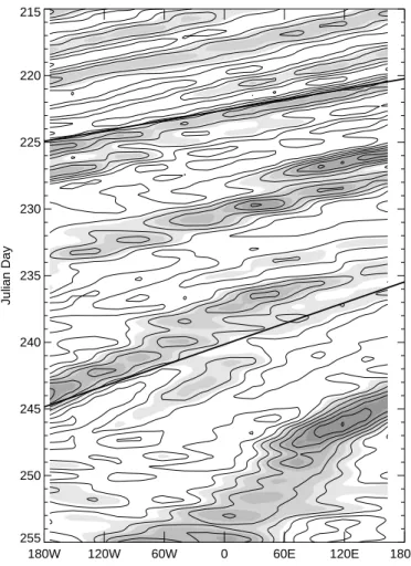
The result of filtering the waves with short zonal and temporal scales is shown for one pressure level in Figs.1and2. The Hovmoller plots for temperature and nitrous oxide at

15

∼62 km altitude for the period 1 August to 15 September clearly show a wavenumber 1 wave with a westward phase propagation. Both methane and ozone exhibit similar behaviour. (Results not shown.) Overlaid on these plots are the phase lines for waves with periods of 5 and 10 days. All fields clearly show a wavenumber 1 wave with a period of 5–7 days in mid- to late August (Julian days 220–235). The period then

20

migrates to a period closer to 10 days by late August to early September (Julian days 240–245), and by mid-September is closer to 16 days for nitrous oxide.

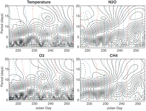
Because of the variation of the wave period, spectral analysis was done using Fourier decomposition in the zonal direction, taking only wavenumber 1, and then using wavelet decomposition in time with a Morlet wavelet of order 3. The wavelet analysis is shown

25

in Fig.3 for all fields at 62 km. In all four fields, waves with periods of approximately 5–7 days are present at the beginning of August, in agreement with the Hovmoller

(7)

ACPD

7, 12011–12033, 2007

Full Screen / Esc

plots. By mid-September, the wave in both temperature and ozone has both weakened in amplitude, and lengthened in period to about 7 days, with some power at longer periods. For nitrous oxide and methane, the amplitude has weakened and the period has lengthened to almost 16 days by mid-September.

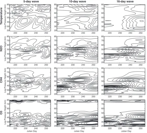
In order to look at the vertical distribution of the wave amplitudes, the Fourier-wavelet

5

decomposition was integrated over a frequency range for each wave (5, 10 and 16 day). For the 5-day wave the range was 1.37–0.97 cpd (4.6 to 6.5 days), for the 10-day wave 0.68–0.53 cpd (9.2 to 11.9 days), and for the 16-day wave 0.44–0.34 cpd (14.1 to 18.3 days). The results are shown in Fig.4. In temperature, all three waves have max-imum amplitudes between 40 to 50 km with secondary maxima above 70 km. Similar

10

behaviour is seen in nitrous oxide and methane, although the frequency separation between the 5, 10 and 16 day waves is less clear. Because the MANTRA campaign measures at altitudes ranging from 10 km to 50 km, we will focus on the maxima near 50 km. The 10- and 16-day waves also develop later in the summer than the 5-day wave.

15

Some care must be taken in interpreting these results since the wavelet analysis tends to broaden spectral peaks compared to the more common Fourier analysis, so that some signal is evident in the 10-day wave earlier in the summer, although the peak amplitude in Fig.3is clearly not at 10 days. In addition, the period of the wave during early August is somewhat longer than 5 days, adding to the problem of interpreting this

20

as part of the 10-day wave. Furthermore, because the frequency range for the 16-day wave is broad and the evolution of the amplitude between solstice and equinox is similar to the 10-day wave, it is sometimes difficult to distinguish between the two.

The zonal-mean zonal wind at 52.6◦N may provide some explanation for the migra-tion of the wave frequency. Figure5shows the zonal-mean zonal wind evolution over

25

the late summer period. Also shown are the critical lines, where ¯_{u−c=0, for waves} with zonal wavenumber 1 and periods of 5, 10 and 16 days. Rossby waves exhibit westward phase propagation relative to the background flow so that a wave of a given period may exist only where ¯u>c, or in the case of the summer easterly jet, where c is

(8)

ACPD

7, 12011–12033, 2007

Full Screen / Esc

EGU

more negative than ¯u. As suggested byGeisler and Dickinson(1976) andPrata(1989) for the 5-day wave, the waves become vertically trapped by the easterly jet. As the wind approaches turnaround, the summer easterly jet is reduced in magnitude and is squeezed in vertical extent, providing a deeper resonant cavity. As demonstrated in Fig.5, the area of allowed propagation (below the critical levels) is largest for the 5-day

5

wave, and smallest for the 16-day wave, growing over the season as the jet weakens. Waves above the critical levels are expected to be evanescent.

3.1 Correlations

Despite the difficulties in interpreting Fig.4, there is clearly some correlation between the fields for the different waves.

10

The time-lagged correlations for both the spatial fields, and the amplitudes of the 5-day, 10-day and 16-day waves are presented here. Statistical confidence levels were calculated using the method outlined bySciremammano(1979).

Since both CH₄ and N₂O have sources in the troposphere, and are oxidized in the stratosphere, where neither has significant sources, it is expected that they will

15

be well-correlated at all altitudes below a certain level. Where time scales of atmo-spheric mixing are much shorter than photochemical lifetimes, CH₄ and N₂O distri-butions should exhibit a compact correlation. Even where horizontal mixing is rapid compared to vertical mixing, as in the stratosphere, correlations should vary only with altitude (Michelsen et al.,1998). This is seen in the CMAM results as methane and

ni-20

trous oxide are well-correlated at the 95% confidence level at all altitudes below 65 km with zero time-lag (not shown), with correlations decreasing with altitude. Even above 65 km, the fields are well-correlated at the 90% confidence level.

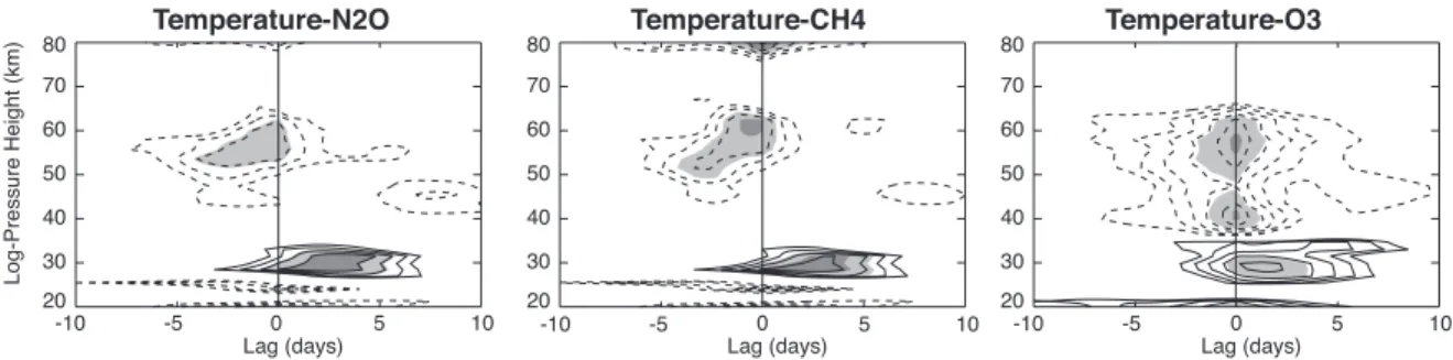
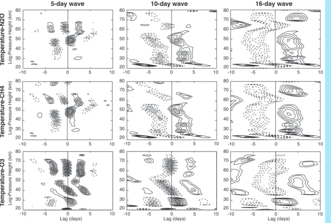
Time-lagged correlations of temperature vs. nitrous oxide, methane and ozone are shown in Fig.6. Where the time-lag is positive, the changes in the temperature lead

25

changes in the chemical fields, and where the time-lag is negative, the chemical fields lead temperature. However, due to the periodic nature of the 5, 10 and 16 day waves, causality is not implied by the sign of the lag. In all correlation plots, a positive

(9)

correla-ACPD

7, 12011–12033, 2007

Full Screen / Esc

tion at∼2 days lead for temperature between 28 and 33 km: an increase in temperature corresponds to an increase in nitrous oxide, methane and ozone approximately 2 days later. This corresponds to an altitude region where chemical lifetimes of these species (months for ozone, several years for methane and nitrous oxide) are longer than trans-port time scales, and therefore transtrans-port is expected to be dominant in controlling the

5

chemical distributions. Further investigation reveals that the correlation in this region is likely due to meridional transport; the chemical fields are negatively correlated with meridional wind at these levels at the 95% confidence level.

Above these altitudes, where chemical lifetimes are shorter, chemistry becomes more important. Ozone, which has a lifetime of several hours at these altitudes, is

10

anti-correlated with temperature with a zero time-lag, suggesting that it adjusts almost simultaneously to the temperature in this region: an increase in temperature produces a simultaneous decrease in ozone due to an increase in ozone destruction. The role of chemistry should be less important for nitrous oxide and methane, which both have lifetimes of several months at these altitudes. For these species, increases in nitrous

15

oxide and methane lead decreases in temperature, up to 3 days later at 50 km.

Time-lagged correlations for the 5, 10 and 16 day waves as calculated for Fig.4are shown in Fig.7, using both amplitude and phase information. The periodicity of the time series are clearly reflected in the periodic nature of the correlations. Also, because of the longer autocorrelation of the 10 and 16 day wave time series, the significance level

20

of the cross-correlations is reduced. In fact, for the 16 day wave, there are no significant cross-correlations. This is also due partly to the shorter duration of the 16 day wave signal in the data set. Caution must also be used in interpreting these results. For example, although there appears to be a significant correlation between temperature and nitrous oxide and ozone at 60 km with a time-lag of –1 day, the amplitude of the

25

10-day wave is very small at this altitude. Therefore, although there may be significant correlations, the 10-day wave may not significantly affect the chemical concentrations in an absolute sense in this region.

(10)

ACPD

7, 12011–12033, 2007

Full Screen / Esc

EGU

temperature leads an increase in N₂O and CH₄ one day later, and an increase in temperature lags a decrease in N2O and CH4approximately 2–3 days later. For ozone, the simultaneous increase in temperature and decrease in ozone corresponding to Fig.6is present, along with a positive correlation at±2–3 days, reflecting the periodicity of the wave. Similar behaviour is seen in the 10-day wave correlations, although with

5

slightly longer lead and lag times (up to 5 days in the case of temperature vs. ozone). Correlations with the zonal and meridional winds (not shown) suggest that the links between temperature and nitrous oxide and methane are largely due to horizontal transport between 30 and 60 km. While the meridional wind is better correlated with the chemical fields than the zonal wind, suggesting that meridional transport by the waves

10

may be more important, this cannot be further tested with the existing data set. Vertical transport may also play a role in determining the relationship between the waves and the chemical species, but also cannot be tested with the existing data set. The rela-tionship between temperature and ozone for the waves appears to be partly through transport and partly through a chemical balance between temperature and ozone. It

15

should be noted that no correlations between waves in the zonal and meridional winds and those in the chemical fields were evident at 25–30 km, suggesting that the effect of transport in this region may be due to the zonal-mean meridional transport, although again, vertical transport may be partly responsible.

4 Interannual variability

20

Although the 5-day, 10-day and 16-day waves are resonant modes of the atmosphere, all are expected to exhibit some interannual variability since the resonant properties of the atmosphere change with varying background winds and temperatures, which them-selves show interannual variability. In order to characterize the interannual variability of the waves, model data from 24 years of the climate run sampled at 18 h intervals

25

on five pressure levels for the months of August and September were used. Because the sampling interval was coarser, the prominent diurnal cycle associated with the tide

(11)

ACPD

7, 12011–12033, 2007

Full Screen / Esc

seen in the data set with higher temporal sampling was not present, and no filtering was needed. The Fourier-wavelet decomposition as described in Sect. 3 was used to iso-late the waves, and amplitudes were again integrated over period ranges 4.6–6.5 days (5-day wave), 8.4–10.9 days (10-day wave) and 14.2–18.4 days (16-day wave). The ranges are slightly different than those used in the previous data set because of the

5

different sampling interval, which produces different frequency intervals in the wavelet analysis. Only the highest altitudes are shown since the waves are harder to isolate on the 100 mb and 60 mb pressure surfaces.

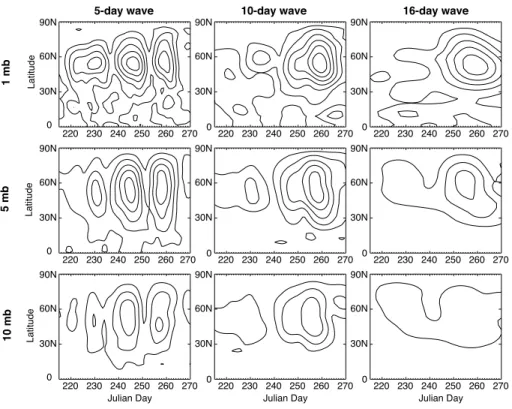
Results for a typical year are shown in Fig.8. In this year, all three waves are present with approximately the same amplitudes, although the 10-day and 16-day waves

de-10

velop later in the summer. For all years, the amplitudes are maximum near 50◦N, although the time evolution can be very different. The lobed structure of the time evo-lution of the 5-day wave is common, although in some years the amplitude decreases more rapidly in September. The later development of the 16-day wave is also common, although not universal. The 10-day wave, however, shows greater variation in both

15

timing and amplitude.

To examine the year-to-year variability of the waves, the amplitudes were integrated over the latitude range 39◦N to 72◦N. The results are shown in Fig.9. Although the amplitude is never zero for any wave in any year, in some cases the amplitudes remain

<1 K, and in other years one wave may dominate over the other two. For both the 10

20

and 16 day waves, the amplitude tends to grow steadily over the summer, whereas the 5-day wave shows the greatest variation in timing from year-to-year. In some years the amplitude is large in early August, and in some is it largest in late September. In other years, the amplitude fluctuates over the entire period. For the 16-day wave, the am-plitude starts relatively small in all years, growing to a maximum amam-plitude later in the

25

summer before eventually decaying. This is expected from the behaviour of the normal mode as calculated by Salby(1981). The 10-day wave has the greatest amplitudes, and tends to be strongest from late August to early September, although showing the strongest variation in timing. As noted earlier, interpretation of the 10-day wave is

(12)

ACPD

7, 12011–12033, 2007

Full Screen / Esc

EGU

difficult because of the overlap of periods between it and the 5 and 16 day waves.

5 Discussion and conclusions

Using the CMAM, a fully-interactive coupled-chemical GCM, the normal mode Rossby waves for the 5, 10 and 16 day waves in both the temperature and chemical fields have been analysed. All fields are shown to have 5,10 and 16 day waves. (It should be noted

5

that NOy, a long-lived chemical family, was also analysed but did not appear to contain a clear signature of the waves.) There is a clear correlation between the temperature, nitrous oxide, methane and ozone, both in real space and when the correlations for each wave are considered. Below 30 km, temperature and the chemical fields are well-correlated with a lead of 2–3 days. This may be the result of mean meridional transport

10

in the stratosphere, which although weak in the summer hemisphere, nevertheless exists (Cordero and Kawa,2001).

The 5-day and 10-day waves in temperature and the chemical fields are well-correlated between 30 km to 60 km, suggesting that these normal modes may have a significant effect on chemical concentrations. This effect seems to be the result of

15

horizontal transport in the region due to the waves. Vertical transport may also play a role, but could not be tested here. Because of the shorter lifetime of ozone at these altitudes, ozone most likely also respond directly to the 5 and 10 day waves in tem-perature. While correlations exist between temperature and the chemical fields for the 16-day wave, they are not statistically significant due to the short duration of the wave

20

and the limited time series.

An examination of the interannual variability of the 5, 10 and 16 day waves shows that these waves could, and likely do, exist during the MANTRA campaigns in August and September. Which waves are most likely present would depend to some extent on the timing of the launch – launches later in the summer are more likely to see longer

25

period waves – and on the particular year. Ground-based measurements or tempera-ture analyses supporting the balloon measurements may be necessary to provide the

(13)

ACPD

7, 12011–12033, 2007

Full Screen / Esc

phase and amplitude of the waves during the balloon launch. Data analyses could also provide the meridional structure of the waves, and more clearly identify which modes are present. Since MANTRA balloon measurements are taken for only one day at a time, the effect of the waves on the chemical species must be taken into account in order to determine long-term trends in the species.

5

Further study with global data at a finer sampling interval would be useful for several reasons. First, the choice of frequency separation between the 5, 10 and 16 day waves in this study was somewhat arbitrary, based only on the frequency variations calculated bySalby(1981). This is not ideal since, as seen in Fig.3, the 5-day wave in the CMAM is skewed towards longer periods in the allowable frequency range. In addition, the

10

frequency range for the 16-day wave can overlap that of the 10-day wave making it difficult to properly distinguish between the two. Since all three of the wavenumber 1 normal modes have maximum amplitudes near 50◦N, the meridional phase structure is the only way to truly distinguish between them. With only one latitude in the data set with the high temporal sampling, it is impossible to determine the meridional structure

15

of the waves, which can help to identify the normal modes. In the case of the global data, the temporal and vertical resolution of the data is insufficient to obtain definitive phase structures.

References

Beagley, S. R., de Grandpr ´e, J., Koshyk, J. N., McFarlane, N. A., and Shepherd, T. G.:

20

Radiative-dynamical climatology of the first-generation Canadian Middle Atmosphere Model, Atmos.-Ocean, 35, 293–331, 1997. 12014

Brasseur, G. and Solomon, S.: Aeronomy of the Middle Atmosphere, D. Reidel, 1986.

Cheong, H.-B. and Kimura, R.: Excitation of the 5-day Wave by Antarctica, J. Atmos. Sci., 54, 87–102, 1997.12013

25

Cheong, H.-B. and Kimura, R.: Excitation of the 10-day and 14-day waves, J. Atmos. Sci., 58, 1129–1145, 2001.

(14)

ACPD

7, 12011–12033, 2007

Full Screen / Esc

EGU

Cordero, E. C. and Kawa, S. R.: Ozone and tracer transport variations in the summer Northern Hemisphere stratosphere, J. Geophys. Res., 106, 12 227–12 240, 2001.12021

de Grandpr ´e, J., Beagley, S. R., Fomichev, V. I., Griffioen, E., McConnell, J. C., Medvedev, A. S., and Shepherd, T. G.: Ozone climatology using interactive chemistry: Results from the Canadian Middle Atmosphere Model, J. Geophys. Res., 105, 26 475–26 491, 2000. 12014

5

Geisler, J. E. and Dickinson, R. E.: The Five-Day Wave on a Sphere with Realistic Zonal Winds, J. Atmos. Sci., 33, 632–641, 1976.12013,12017

Hines, C. O.: Doppler-spread parameterization of gravity-wave momentum deposition in the middle atmosphere. Part 1: Basic formulation, J. Atmos. and Solar-Terr. Phys., 59, 371–386, 1997. 12014

10

Hirooka, T.: Normal Mode Rossby Waves as Revealed by UARS/IASMS Observations, J. At-mos. Sci., 57, 1277–1285, 2000.

Hirooka, T. and Hirota, I.: Further Evidence of Normal Mode Rossby Waves, Pageoph., 130, 277–289, 1989. 12013

Hirota, I. and Hirooka, T.: Normal Mode Rossby Waves Observed in the Upper Stratosphere.

15

Part I: First Symmetric Modes of Zonal Wavenumbers 1 and 2, J. Atmos. Sci., 41, 1253– 1267, 1983. 12013

Madden, R. and Julian, P.: Further Evidence of Global-Scale, 5-Day Pressure Waves, J. At-mos. Sci., 29, 1464–1469, 1972. 12013

Madden, R. A.: Further Evidence of Traveling Planetary Waves, J. Atmos. Sci., 35, 1605–1618,

20

1978.

McLandress, C.: On the importance of gravity waves in the middle atmosphere and their param-eterization in general circulation models, J. Atmos. Sol.-Terr. Phys., 60, 1357–1383, 1998.

12014

McLandress, C.: Interannual variations of the diurnal tide in the mesosphere induced by

zonal-25

mean wind oscillations in the tropics., Geophys. Res. Lett., 29, doi:10.1029/2001GL014 551, 2002. 12015

Michelsen, H. A., Manney, G. L., Gunson, M. R., Rinsland, C. P., and Zander, R.: Correla-tions of stratospheric abundances of CH₄ and N₂O derived from ATMOS measurements, Geophys. Res. Lett., 25, 2777–2780, 1998. 12017

30

Miyoshi, Y.: Numerical simulation of the 5-day and 16-day waves in the mesopause region, Earth Planets Space, 51, 763–772, 1999.

(15)

ACPD

7, 12011–12033, 2007

Full Screen / Esc

GCM, J. Atmos. Sci., 56, 1698–1707, 1999.12013

Prata, A. J.: Observations of the 5-Day Wave in the Stratosphere and Mesosphere, J. At-mos. Sci., 46, 2473–2477, 1989. 12013,12017

Salby, M. L.: Rossby Normal Modes in Nonuniform Background Configurations. Part II: Equinox and Solstice Conditions, J. Atmos. Sci., 38, 1827–1840, 1981.12013,12020,12022

5

Sciremammano, F. J.: A suggestion for the Presentation of Correlations and their significance levels, J. Phys. Ocean., 9, 1273–1276, 1979. 12017

(16)

ACPD

7, 12011–12033, 2007

Full Screen / Esc

EGU

180W 120W 60W 0 60E 120E 180E

255 250 245 240 235 230 225 220 215 Julian Day

Fig. 1. Hovmoller plot of temperature filtered to allow waves with periods greater than 1.2 days

and zonal wavenumbers less than 5 at 62 km and 52.6◦N. Contour intervals are 1.2 K and higher values are shaded. Overlaid are the phase lines for a wave with period 5 days (top) and 10 days (bottom).

(17)

ACPD

7, 12011–12033, 2007

Full Screen / Esc

180W 120W 60W 0 60E 120E 180E

255 250 245 240 235 230 225 220 215 Julian Day

(18)

ACPD

7, 12011–12033, 2007

Full Screen / Esc

Printer-friendly Version Interactive Discussion EGU 220 230 240 250 Julian Day 0 5 10 15 20 Period (days) 220 230 240 250 Julian Day 0 5 10 15 20 220 230 240 250 0 5 10 15 20 Period (days) 220 230 240 250 0 5 10 15 20 Temperature N2O CH4 O3

Fig. 3. Fourier-wavelet decomposition for temperature (top-left panel), nitrous oxide (top-right

panel), ozone (bottom-left panel) and methane (bottom-right panel) at 62 km and 52.6◦N. Contour intervals are 0.26 K/km/cpd for temperature, 0.01 ppbv/km/cpd for nitrous oxide, 7.8 ppbv/km/cpd for methane, and 2.6 ppbv/km/cpd for ozone. Phase lines are overlaid on each plot for phases 0 (dashed-black), 90 (dashed-blue), 180 (dashed-red) and 270 (dashed-green). Minima in amplitude are easily distinguished by the convergence of phase lines through them.

(19)

ACPD

7, 12011–12033, 2007

Full Screen / Esc

Printer-friendly Version Interactive Discussion 220 230 240 250 20 30 40 50 60 70 80 Log-Pressure Height (km) 220 230 240 250 20 30 40 50 60 70 80 220 230 240 250 20 30 40 50 60 70 80 220 230 240 250 20 30 40 50 60 70 80 Log-Pressure Height (km) 220 230 240 250 20 30 40 50 60 70 80 220 230 240 250 20 30 40 50 60 70 80 220 230 240 250 20 30 40 50 60 70 80 Log-Pressure Height (km) 220 230 240 250 20 30 40 50 60 70 80 220 230 240 250 20 30 40 50 60 70 80 220 230 240 250 Julian Day 20 30 40 50 60 70 80 Log-Pressure Height (km) 220 230 240 250 Julian Day 20 30 40 50 60 70 80 220 230 240 250 Julian Day 20 30 40 50 60 70 80 T emperature N2O CH4 O3

5-day wave 10-day wave 16-day wave

Fig. 4. Fourier-wavelet decomposition showing altitude vs. time for temperature (top row),

nitrous oxide (second row), methane (third row), and ozone (bottom row) for the 5-day wave (left column), 10-day wave (middle column) and 16-day wave (right column). Contour inter-vals are 1.5 K/km/cpd for temperature, 0.18 ppmv/km/cpd for nitrous oxide, 37 ppbv/km/cpd for methane and 75 ppbv/km/cpd for ozone. Nitrous oxide has been scaled by a density factor of

(20)

ACPD

7, 12011–12033, 2007

Full Screen / Esc

Printer-friendly Version Interactive Discussion EGU 220 230 240 250 Julian Day 20 40 60 80 100 Log-Pressure Height (km) 5 5 5 10 10 10 16 16 16 16

Fig. 5. The zonal-mean zonal wind at 52.6◦N from 1 August to 15 September. Contour levels are 5 m/s and reach a minimum of –73.3 m/s. Thick black lines represent the critical lines for planetary waves with zonal wavenumber one and periods of 5, 10 and 16 days, labelled accordingly.

(21)

ACPD

7, 12011–12033, 2007

Full Screen / Esc

Printer-friendly Version Interactive Discussion 0 Lag (days) 20 30 40 50 60 70 80 Log-Pressure Height (km) 0 Lag (days) 20 30 40 50 60 70 80 0 Lag (days) 20 30 40 50 60 70 80

Temperature-N2O Temperature-CH4 Temperature-O3

-10 -5 5 10 -10 -5 5 10 -10 -5 5 10

Fig. 6. Time-lagged correlations of temperature and nitrous oxide (left panel), temperature and

methane (middle panel), and temperature and ozone (right panel). Contours are 0.05 and are shown only for|CorXY(τ)|≥0.5. Significance levels for the 90% (light gray), 95% (medium gray)

(22)

ACPD

7, 12011–12033, 2007

Full Screen / Esc

Printer-friendly Version Interactive Discussion EGU -10 -5 0 5 10 20 30 40 50 60 70 80 Log-Pressure Height (km) 20 30 40 50 60 70 80 20 30 40 50 60 70 80 20 30 40 50 60 70 80 Log-Pressure Height (km) 20 30 40 50 60 70 80 20 30 40 50 60 70 80 Lag (days) 20 30 40 50 60 70 80 Log-Pressure Height (km) 20 30 40 50 60 70 80 Lag (days) 20 30 40 50 60 70 80

T emperature-N2O T emperature-CH4 T emperature-O3 -10 -5 0 10 -10 -5 0 5 10 -10 -5 0 5 10 -10 -5 0 5 10 -10 -5 0 10 -10 -5 0 5 10 -10 -5 0 5 10 -10 -5 0 5 10 5 5 Lag (days)

Fig. 7. Similar to Fig.6but for correlations between temperature-N₂O (top row), temperature-CH₄(middle row) and temperature-O₃(bottom row) for the 5-day (left column), 10-day (middle column) and 16-day waves (right column). Significance levels for the 90% (light gray), 95% (medium gray) and 99% (dark gray) are shown.

(23)

ACPD

7, 12011–12033, 2007

Full Screen / Esc

Printer-friendly Version Interactive Discussion 220 230 240 250 260 270 0 30N 60N 90N 220 230 240 250 260 270 0 30N 60N 90N 220 230 240 250 260 270 0 30N 60N 90N 220 230 240 250 260 270 0 30N 60N 90N 220 230 240 250 260 270 0 30N 60N 90N 220 230 240 250 260 270 0 30N 60N 90N 220 230 240 250 260 270 Julian Day 0 30N 60N 90N 220 230 240 250 260 270 Julian Day 0 30N 60N 90N 220 230 240 250 260 270 Julian Day 0 30N 60N 90N Latitude Latitude Latitude

1 mb

5 mb

10 mb

Fig. 8. Temperature amplitudes as calculated for Fig.4, but for year 17 of the climate run. Amplitudes are shown for the NH only for the 5-day wave (left column), 10-day wave (middle column), and 16-day wave (right) column for pressure levels 1 mb (∼48 km) (top row), 5 mb (∼35 km)(middle row) and 10 mb (∼32 km) (bottom row). Contour intervals are 0.5 K/km/cpd in all panels.

(24)

ACPD

7, 12011–12033, 2007

Full Screen / Esc

Printer-friendly Version Interactive Discussion EGU 0.5 1.0 1.5 2.0 2.5 3.0 Amplitude (K) 0.5 1.0 1.5 2.0 2.5 3.0 Amplitude (K) 220 230 240 250 260 270 Julian Day 0.0 0.5 1.0 1.5 2.0 2.5 3.0 Amplitude (K) 0.5 1.0 1.5 2.0 2.5 3.0 0.5 1.0 1.5 2.0 2.5 3.0 220 230 240 250 260 270 Julian Day 0.0 0.5 1.0 1.5 2.0 2.5 3.0 0.5 1.0 1.5 2.0 2.5 3.0 0.5 1.0 1.5 2.0 2.5 3.0 220 230 240 250 260 270 Julian Day 0.0 0.5 1.0 1.5 2.0 2.5 3.0

1 mb

5 mb

10 mb

Fig. 9. Temperture amplitudes integrated over latitude for all 24 years of the climate run for

the 5-day wave (left column), 10-day wave (middle column), and 16-day wave (right) column for pressure levels 1 mb (top row), 5 mb (middle row) and 10 mb (bottom row). The 24-year average is indicated by the thick dark line in each panel.