HAL Id: hal-01851031
https://hal.archives-ouvertes.fr/hal-01851031
Submitted on 28 Jul 2018
HAL is a multi-disciplinary open access
archive for the deposit and dissemination of
sci-entific research documents, whether they are
pub-lished or not. The documents may come from
teaching and research institutions in France or
abroad, or from public or private research centers.
L’archive ouverte pluridisciplinaire HAL, est
destinée au dépôt et à la diffusion de documents
scientifiques de niveau recherche, publiés ou non,
émanant des établissements d’enseignement et de
recherche français ou étrangers, des laboratoires
publics ou privés.
Simutė, Lion Krischer, Yeşim Çubuk-Sabuncu, Tuncay Taymaz, Lorenzo Colli,
Erdinc Saygin, Antonio Villaseñor, et al.
To cite this version:
Andreas Fichtner, Dirk-Philip van Herwaarden, Michael Afanasiev, Saulė Simutė, Lion Krischer, et
al.. The Collaborative Seismic Earth Model: Generation 1. Geophysical Research Letters, American
Geophysical Union, 2018, 45 (9), pp.4007-4016. �10.1029/2018GL077338�. �hal-01851031�
Geophysical Research Letters
The Collaborative Seismic Earth Model: Generation 1
Andreas Fichtner1 , Dirk-Philip van Herwaarden1, Michael Afanasiev1, Saul ˙e Simut ˙e1 ,Lion Krischer1,2, Ye¸sim Çubuk-Sabuncu3, Tuncay Taymaz3 , Lorenzo Colli2,4 , Erdinc Saygin5 , Antonio Villaseñor6 , Jeannot Trampert7 , Paul Cupillard8, Hans-Peter Bunge2 ,
and Heiner Igel2
1Department of Earth Sciences, ETH Zurich, Zurich, Switzerland,2Department of Earth and Environmental Sciences, LMU Munich, Munich, Germany,3The Faculty of Mines, Department of Geophysical Engineering, Istanbul Technical University, Istanbul, Turkey,4Department of Earth and Atmospheric Sciences, University of Houston, Houston, TX, USA, 5School of Physics and Astrophysics, University of Western Australia, Perth, Australia,6Institute of Earth Sciences Jaume Almera, ICTJA-CSIC, Barcelona, Spain,7Department of Earth Sciences, Utrecht University, Utrecht, The Netherlands, 8GeoRessources, University of Lorraine/CNRS, Vandoeuvre-lès-Nancy, France
Abstract
We present a general concept for evolutionary, collaborative, multiscale inversion of geophysical data, specifically applied to the construction of a first-generation Collaborative Seismic Earth Model. This is intended to address the limited resources of individual researchers and the often limited use of previously accumulated knowledge. Model evolution rests on a Bayesian updating scheme, simplified into a deterministic method that honors today’s computational restrictions. The scheme is able to harness distributed human and computing power. It furthermore handles conflicting updates, as well as variable parameterizations of different model refinements or different inversion techniques. The first-generation Collaborative Seismic Earth Model comprises 12 refinements from full seismic waveform inversion, ranging from regional crustal- to continental-scale models. A global full-waveform inversion ensures that regional refinements translate into whole-Earth structure.Plain Language Summary
Modern geophysical data are often characterized by their distribution across multiple spatial scales, meaning that high-density local or regional deployments are complemented by coarser global-scale recordings. Examples include data from seismic, electromagnetic, or Global Positioning System (GPS) measurements. While data volumes increase steadily, the actually usable amount of information is limited by the available human and computing power of individual researchers. Here we present a new framework that supports collaborative and evolutionary inversion of geophysical data, where prior knowledge from earlier data can be incorporated. We exemplify our method with a seismological application, that is, the construction of a Collaborative Seismic Earth Model of the 3-D internal structure of our planet.1. Introduction
1.1. Evolving Multiscale Data and Inversion
Modern geophysical data are often characterized by their distribution across multiple spatial scales, mean-ing that high-density local or regional deployments are complemented by coarser global-scale recordmean-ings. Examples include data from seismic (e.g., Díaz et al., 2009; Meltzer et al., 1999), electromagnetic (e.g., Chulliat et al., 2017), gravity (e.g., International Gravimetric Bureau [http://bgi.omp.obs-mip.fr]), or Global Positioning System (GPS) (e.g., Kreemer et al., 2014) measurements. While data volumes increase steadily, the actually usable amount of information is limited by the available human and computing power of individual research groups. It therefore becomes increasingly difficult to assimilate all data consistently into one model using modern inversion techniques. The problem may be overcome by an inversion framework that supports collaborative and evolutionary inversion, where prior knowledge from earlier data can be incorporated. Though being only one class of data, seismic recordings exemplify many of these challenges. Seismic data used for tomography are key to understand the Earth’s structure and dynamics (e.g., Bunge et al., 2003; Colli et al., 2017; Koelemeijer et al., 2015; Trampert et al., 2004), explore and monitor reservoirs and volcanoes (e.g., Koulakov et al., 2013; Prieux et al., 2013), characterize earthquakes (e.g., Chen et al., 2007; Hejrani et al., 2017; Liu et al., 2004), and predict the ground motion they induce (e.g., Graves et al., 2010; Lee et al., 2014).
RESEARCH LETTER
10.1029/2018GL077338Key Points:
• We present a framework for evolutionary, community-driven, multiscale inversion of geophysical data
• This is illustrated by the construction of a Collaborative Seismic Earth Model • The first-generation model includes
12 regional refinements based on full-waveform inversion Supporting Information: • Supporting Information S1 Correspondence to: A. Fichtner, andreas.fi[email protected] Citation:
Fichtner, A., van Herwaarden, D.-P., Afanasiev, M., Simut ˙e, S., Krischer, L., Çubuk-Sabuncu, Y., et al. (2018). The Collaborative Seismic Earth Model: Generation 1.
Geophysical Research Letters, 45.
https://doi.org/10.1029/2018GL077338
Received 5 FEB 2018 Accepted 13 APR 2018
Accepted article online 7 MAY 2018
©2018. The Authors.
This is an open access article under the terms of the Creative Commons Attribution-NonCommercial-NoDerivs License, which permits use and distribution in any medium, provided the original work is properly cited, the use is non-commercial and no modifications or adaptations are made.
Performing multiscale tomography is essential, as failure to resolve crustal details may induce artificial anisotropy (Bozda ˘g & Trampert, 2008; Ferreira et al., 2010; Fichtner, Kennett et al., 2013) that may be misinter-preted as mantle flow. While the need to jointly resolve crust and mantle is well recognized, prior knowledge with a level of detail known from crustal studies (e.g., Chen et al., 2007; Tape et al., 2010) is hardly incorpo-rated in (global) tomography (e.g., Bozda ˘g et al., 2016; Koelemeijer et al., 2015; Schaeffer & Lebedev, 2013). The combination of resource limitations and insufficient use of prior knowledge prevent tomography from achieving the ideal of a multiscale model that assimilates the actually available wealth of data. A side effect are discrepancies between models, especially in parameters with strong dependence on small-scale structure, for example, anisotropy and attenuation (Dalton et al., 2008; Ferreira et al., 2010).
1.2. Objectives and Outline
The main objective of this work is the development of an inversion framework that addresses the challenges of evolving multiscale data by meeting the following design criteria: (a) Enable a collaborative and evolutionary model construction to harness distributed human and computing power. (b) Consistently incorporate prior knowledge, accumulated during previous model updates. (c) Allow for variable parameterizations of different model refinements and of potentially different inversion techniques.
In section 2 we present the methodological developments, using the example of a Collaborative Seismic Earth Model (CSEM) for illustration. This includes the construction of an initial model, a Bayesian updating scheme for evolutionary multiscale refinement, pragmatic simplifications demanded by current computational limi-tations, and the handling of apparently conflicting updates. Following the general developments, we more specifically consider the first-generation CSEM in section 3, which comprises 12 refinements from full seismic waveform inversion, ranging from regional crustal to global scales.
2. Evolutionary, Collaborative, Multiscale Inversion
In the following, we present a scheme for evolutionary, collaborative, multiscale inversion. It is designed to ensure computational efficiency, easy handling, completeness and flexibility of the parametrization, a clean refinement procedure, and the ability to handle both successive and simultaneous updates. Though being per se application independent, the general development is exemplified by the CSEM, which serves as a large-scale use case that allows us to identify bottlenecks. In this context, we abandoned an earlier prototype based on a whole-Earth refinable tetrahedral mesh (Afanasiev et al., 2016). While elegant in theory, it was too difficult to handle in practice, already requiring supercomputing resources for trivial tasks such as visualization and the addition of a refinement region.
2.1. Initial Model
We begin with the construction of an initial model. A physical parameter of the initial model ̂m0as a function
of position x, for example, an elastic parameter, can be expressed in terms of N0basis functions bi0(x):
̂m0(x) = N0 ∑ i=1 ̂mi 0b i 0(x). (1)
These may include polynomials, spherical harmonics, blocks, or a combination of these. The initial model vector ̂m0= (̂m1
0, … , ̂m
N0
0 )Tis the maximum-likelihood model of the prior probability density function (pdf ),
p0(m0), the shape of which will be specified in section 2.3.
In the specific context of the CSEM, the initial model is designed to be conservative in the sense of not con-taining structure that seismic data cannot modify, while still matching our longest-period data to within half a cycle. It is built upon Preliminary Reference Earth Model (PREM; Dziewo ´nski & Anderson, 1981). Since PREM’s 220-km discontinuity has been suggested to be only a regional feature (e.g., Gu et al., 2001), it is replaced by a linear gradient, as shown in Figures S2 and S3 in the supporting information. Superimposed are the S veloc-ity variations of S20RTS (Ritsema et al., 1999), to which P velocveloc-ity variations are scaled (Ritsema & van Heijst, 2002). The crust of PREM is replaced by the crustal model of (Meier et al., 2007), derived from surface wave inversion. Images of the initial model are presented in Figures S5 to S16.
Since bandlimited data can only constrain smooth, effective versions of discontinuities (Capdeville et al., 2013), we implemented the initial Moho as a gradient over ∼5 km, derived from the original crustal model by Backus averaging (Backus, 1962). This choice ensures that the effective sharpness of the Moho and thickness
Geophysical Research Letters
10.1029/2018GL077338
of the crust can be simply adjusted by not making an explicit distinction between crust and mantle during the inversion.
2.2. Model Parametrization and Bayesian Regional Updating
From the initial model the CSEM evolves through regional refinements that can be described within a rigor-ous Bayesian framework. While computational limitations currently enforce pragmatic simplifications (section 2.3), the idealistic Bayesian approach defines possible future improvements and offers solutions to emerging issues, such as simultaneous updates within overlapping regions.
The construction of a regionally refined version m1(x) of m0(x) starts with the addition of N1basis functions bi
1(x) to the initial model representation,
m1(x) = N0 ∑ i=1 mi 0b i 0(x) + N1 ∑ i=1 mi 1b i 1(x). (2)
The coefficient vector m1of the new basis functions may, for example, represent smaller-scale variations
rel-ative to the initial model. They are initially constrained by the prior p0(m1|m0), which is conditioned on the
initial model itself because the probability of newly added variations depends on the structure that is already present. The prior contains, for instance, parameter correlations derived from mineral-physics arguments or information on the allowable variations relative to the initial model. Through the assimilation of additional regional data, d1, we obtain a conditional likelihood function L0(m1|m0). Combining prior and likelihood via Bayes’ theorem, yields the conditional posterior for the variations m1,
p(m1|m0) = k p0(m1|m0)L0(m1|m0), (3)
with normalization factor k. While both likelihood and posterior depend on d1, this is omitted in the interest of a more succinct notation, especially in later developments. The joint posterior for the initial model coefficients
m0and the variations m1follows from the conjunction of the conditional posterior p(m1|m0) with the initial
model prior p0(m0),
p(m0, m1) = p(m1|m0)p0(m0). (4)
This process can be iterated using p(m0, m1) as new prior, adding basis functions with coefficients m2for
further refinement with a new data set d2, and then using Bayes’ theorem and the conjunction of pdfs to
obtain the next posterior or next state of the CSEM, p(m0, m1, m2). The basis functions of different refinements need not be the same.
The geometric parametrization of the CSEM differs strongly from the earlier prototype, defined on a large, regionally refined, tetrahedral mesh (Afanasiev et al., 2016). Each regional refinement ̂mnretains its genuine basis functions bi
n(x) used during its construction. The CSEM is thus a library of continuously defined updates
that are assembled when the elastic properties of the Earth at some position x are queried. A set of positions may then be used for visualization or as grid points in a numerical wave propagation solver. The main benefits of the library versus the large, single mesh are greater flexibility in removing and adding refinement regions, as well as vastly reduced computational requirements for visualization and the extraction of submodels. 2.3. Pragmatic Simplifications
To avoid the computationally unfeasible sampling of high-dimensional model spaces, the pure Bayesian approach requires simplifications. The first of these consists in the assumption that all pdfs are Gaussian, described by a mean and a covariance. The mean, or equivalently the maximum-likelihood model ̂m1of
p(m1|m0), is then not computed via Bayes’ theorem, as in equation (3), but approximated by minimizing a
quadratic misfit functional𝜒, starting from the maximum-likelihood initial model ̂m0. Repeating the process
leads to the representation of the current state’s maximum-likelihood model in terms of a sum of successive regional refinements, as illustrated in Figure 1.
The Hessian H of𝜒 evaluated at ̂m1 equals the inverse covariance, C−11 of the posterior p(m1|m0). While H cannot be computed or stored explicitly, computationally manageable approximations can be estimated
(e.g., Bui-Thanh et al., 2013; Fichtner & Trampert, 2011a; Fichtner & van Leeuwen, 2015). Furthermore, arbi-trary Hessian-vector products can be evaluated efficiently using second-order adjoints (e.g., Fichtner & Trampert, 2011b; Santosa & Symes, 1988), which is sufficient for uncertainty analysis and gradient-based optimization schemes.
Figure 1. Technical implementation and updating of the CSEM. (a) Schematic illustration of successive refinements, ̂m1, ̂m2,…, being added to the smooth maximum-likelihood initial model ̂m0. Each update is treated as a new item in an ordered library, keeping the parametrization used during its construction. Different updates may be parametrized differently, that is, have different types of basis functions. (b) Concrete example of SV velocity,vsv, at 120-km depth in the
initial model (top) and in the generation-1 model of the CSEM (bottom). Refinement regions visible in this view include Europe, Turkey, the Sea of Marmara region, the North Atlantic, the South Atlantic, and North America. CSEM = Collaborative Seismic Earth Model.
2.3.1. Apparent Inconsistencies and Dependent Updates
In the simplified scheme, the coefficients of already existing basis functions, m0, … , mn, remain unchanged
when a new regional refinement with coefficients mn+1is added. Instead of honoring potential dependencies
of previous on newly added coefficients, the approximation of the maximum-likelihood refinement ̂mn+1is
based on the minimization of a misfit functional with coefficients ̂m0, … , ̂mnas fixed initial model and not
by finding the actual maximum of the joint posterior p(m0, … , mn, mn+1). The approximation error of the
maximum-likelihood model may lead to inconsistencies, meaning that previously assimilated data sets, di≤n
cannot be explained adequately anymore.
The occurrence of simplification-related inconsistencies would in principle require reiterations of previously incorporated refinements. Alternatively, the Gaussian approximation allows us to replace repeated iterations by the solution of a least squares problem. To illustrate the concept, we combine two sets of model param-eters, m′
1and m ′′
1, for instance from successive updates, into a joint parameter vector m1 = (m′1, m ′′ 1). We
then consider two updates with conditional priors p′
0(m1|m0) and p′′0(m1|m0), and with likelihood functions
L′
0(m1|m0) and L′′0(m1|m0), Bayes’ theorem from equation (3) modifies to
p(m1|m0) = k p′0(m1|m0)L′0(m1|m0) p′′0(m1|m0)L′′0(m1|m0). (5)
Within the simplified framework of section 2.3, the maximum-likelihood models, ̂m′
1and ̂m′′1, and
poste-rior covariances, C′
1and C′′1, of the individual posteriors, p′0(m1|m0)L′0(m1|m0) and p′′0(m1|m0)L′′0(m1|m0), are
determined by independent misfit minimizations. It follows that the joint maximum-likelihood model, ̂m1, of
p(m1|m0) is the minimum of − log p(m1|m0) = 1 2(m1− ̂m ′ 1) TC′ 1 −1 (m1− ̂m′ 1) + 1 2(m1− ̂m ′′ 1) TC′′ 1 −1 (m1− ̂m′′ 1) − log k. (6) Noting that C′ 1and C ′′
1are the Hessians H
′and H′′from the independent inversions; ̂m
1can be approximated
iteratively from equation (6) using efficiently computable Hessian-vector products (e.g., Fichtner & Trampert, 2011b; Santosa & Symes, 1988). Rearranging equation (6) and substituting the minimum ̂m1yields the joint
(inverse) posterior covariance,
C−1 1 = C ′ 1 −1 + C′′ 1 −1 = H′+ H′′. (7)
Geophysical Research Letters
10.1029/2018GL077338
Equation (7) indicates that the action of C−1
1 on a model (vector), needed for resolution analysis and further
optimization, is simply the sum of actions of the individual Hessians on the model.
Equations (6) and (7) remove an apparent inconsistency by finding the solution that optimally agrees with the independent updates. While illustrated for updates of the initial model, the equations straightforwardly generalize to later-stage updates of the CSEM, using the concept introduced in section 2.2.
In the current CSEM, described in detail in section 3, no regional refinement has so far led to an apparent incon-sistency that would require the actual execution of the above-derived scheme. This indicates that individual regional refinements indeed tend to improve the CSEM as a whole, at least at the scales that we currently consider. A more detailed discussion of this aspect can be found in section 4.
3. CSEM Generation 1
3.1. Data
The first-generation CSEM includes 12 partially overlapping subregions, refined using three-component waveform data at variable minimum periods, T. These are, in the order in which they have been incorporated, Australasia (T = 40 s; Fichtner et al., 2010), Europe (T = 50 s; Fichtner, Trampert et al., 2013), the North Atlantic (T = 25 s; Rickers et al., 2013), Turkey (T = 10 s; Fichtner, Saygin et al., 2013), the South Atlantic (T = 55 s; Colli et al., 2013), the Western Mediterranean (T = 15 s; Fichtner & Villaseñor, 2015), the wider Japanese Islands region (T = 20 s; Simute et al., 2016), the Iberian Peninsula (T = 8 s), Japan (T = 15 s), North America (T = 30 s), Southeast Asia (T = 20 s), and Western Turkey (T = 8 s; Çubuk Sabuncu et al., 2017). For the Iberian Peninsula and Southeast Asia, we incorporated vertical-component ambient noise correlations, working under the sim-plifying assumption that correlations are proportional to interstation Rayleigh wave Green’s functions (e.g., Lobkis & Weaver, 2001; Wapenaar & Fokkema, 2006).
To ensure consistency of regional refinements that do not overlap with previous ones, we incorporate three-component waveforms from 223 events recorded globally by 149 high-quality broadband stations at T = 55 s. The global data, assimilated between the updates in the Japanese Islands and the Western Mediter-ranean, translate the effects of regional refinements into improved whole-Earth structure. As illustrated in the supporting information Figure S4, the global-scale update changes S velocities by less than 1% within the uppermost mantle, mostly in response to large regional-scale updates in Eurasia and Australasia.
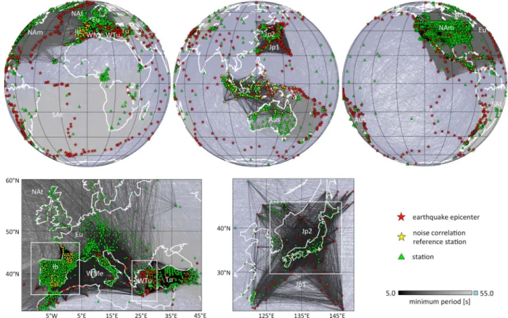
A data summary is presented in Figure 2 in the form of a surface ray density plot. Since full-waveform inver-sion used for the updates exploits a wide range of wave types with different finite-frequency wave paths, ray coverage is only a rough, though useful, proxy for coverage. It illustrates, for instance, that western Europe, Japan, Australasia, and North America are already well covered, whereas the Pacific, central Africa, and central Asia remain to be improved. In total, the current CSEM incorporates waveform data from 948 events (includ-ing virtual events of noise correlations) recorded at 8,975 stations. The total number of source-receiver pairs is 160,797.
3.2. Inversion
To ensure that 3-D wave propagation and finite-frequency effects are properly taken into account, all updates to the CSEM have been performed using full-waveform inversion, following the approach of Fichtner et al. (2010), to which we refer for technical aspects outside the focus of this work. We quantified differences between observed and synthetic seismograms using time-frequency phase misfits (Fichtner et al., 2008), which we reduced iteratively until observations were explained to within the errors or the iteration stalled. To solve the forward and adjoint equations, we employed the spectral-element solvers SPECFEM (Komatitsch & Tromp, 2002a, 2002b) and SES3D (Fichtner et al., 2009; Gokhberg & Fichtner, 2016) at the global and regional scales, respectively. Region-specific inversion details and resolution analyses can be found in the references given in Figure 3.
Since the initial model is not the result of an inversion but an assembly of independent models, a consistent prior p0(m) was not available and thus had to be designed. For simplicity, we set p0(m) to be uniform. For
all subsequent priors, p0(mn+1|m0, … , m1), we chose a covariance that enforces spatial correlation length
scales approximately equal to the minimum wavelength. This common choice prevents the appearance of artifacts that are unlikely to be resolved. In all cases, we did not include correlations between physical model parameters.
Figure 2. Data coverage proxy. Shown are minor-arc great circles connecting earthquake epicenters (red stars) and noise correlation virtual sources (yellow stars) to stations (green triangles). Gray scale represents the minimum period,T, of the waveform data used within a refinement region. Pale blue is used for the global data set withT = 55s. Marked refinement regions are Australasia (Aus), Europe (Eu), Iberian Peninsula (Ib), wider Japanese Islands (Jp1), Japan (Jp2), North America (NAm), North Atlantic (NAt), South Atlantic (SAt), Southeast Asia (SEA), Turkey (Tu), Western Mediterranean (WMe), and Western Turkey (WTu). Refinement regions Ib, JP2, and WTu are marked by a white box for better visibility. The total number of distinct sources (earthquakes plus virtual sources from noise correlations) is 948. With 8,975 distinct stations , they provide 160,797 distinct source-station pairs.
Though the CSEM has flexibility to represent variations in any viscoelastic parameter, we restricted the inver-sions to parameters that are well resolved by the intermediate-period waveform data, that is, P, SH, and SV velocities. Furthermore, we allowed for 3-D density variations in order to avoid artifacts (Blom et al., 2017). Within the lower mantle, the CSEM is practically isotropic, though this has not been enforced explicitly. 3.3. Structural Model
A selection of slices through the SV velocity distribution of the current CSEM are presented in Figure 3. A more comprehensive gallery is shown in the supporting information Figures S5 to S16. Since a geologic interpre-tation is not among the objectives of this work, these are mostly intended to provide an impression of the multiscale nature of the CSEM. The images illustrate the large variation in length scales, ranging from ∼10 km in the crust of Western Turkey to ∼3,000 km in the Central Pacific upper mantle. Most of the significant devi-ations relative to the initial model are confined to the upper 500 km, that is, approximately the maximum penetration depth of regional long-period surface and body waves.
To roughly separate crust and mantle visually, the 15-km slice is shown in a mixed color scale, with gray scale above and colors below 4.0 km/s. The SV velocity distribution is marked by the outline of the continents and the smooth lateral variations of the initial crustal model (Meier et al., 2007). More detailed structure appears where regional-scale shorter-period data (<15 s) have been assimilated, that is, in western Europe, Turkey, and Japan.
From 70- to 200-km depth, the model mostly represents upper-mantle structure, an exception being the Tibetan Plateau. A general feature are anomalous SV velocities below −15%, compared to around −10% in S20RTS (Ritsema et al., 1999). In contrast, the largest positive SV variations of ∼10% are similar to those in S20RTS. While a clear causal relationship between anomalously low velocities, data, and inversion scheme
Geophysical Research Letters
10.1029/2018GL077338
Figure 3. Distribution of SV velocity,vsv, at depths of 15 km (top), 70 km (middle), and 200 km (bottom). At 15-km depth, gray scale roughly corresponds to mantle velocities (4.0–4.8 km/s), and colors from red over white to blue roughly indicate crustal velocities (2.7–4.0 km/s). Key to marked features in regional close-ups: (a) a.KM: Kazda ˘g Massif, a.KVP: Kula Volcanic Province, and a.MM: Menderes Massif; (b) b.JB: Japan Basin, b.SB: Shikoku Basin, and b.TB: Tsushima Basin; (c) c.PB: Pannonian Basin and c.TTL: Tornquist-Teisseyre Line; (d) d.GC: Gawler Craton, d.KB: Kimberley Block, d.NFB: New England Fold Belt, d.PB: Pilbara Block, and d.YB: Yilgarn Block; (e) e.ACS: Apennine-Calabria Slab, e.AS: Alboran Slab, and e.LPB: Liguro-Proven¸al Basin; (f ) f.PS: Pacific Slab, f.PSS: Philippine Sea Slab, and f.UA: Ulleung Anomaly.
is hard to establish, the iterative improvements of full-waveform inversion and its ability to account for wavefront healing are likely to contribute (e.g., Igel & Gudmundsson, 1997; Malcolm & Trampert, 2011; Wielandt, 1987).
4. Discussion and Conclusions
The CSEM is not intended to be a long-wavelength 3-D reference for tomography or a community model in the sense of the Southern California Earthquake Center (SCEC) models (e.g., Small et al., 2017). Instead, it is designed as a framework for successive refinements on all scales and for the consistent use of prior knowledge. As such, it primarily tries to respond to current data and computing challenges, without claiming to be the only possible solution.
The updating scheme from section 2.2 is the foundation upon which the CSEM operates. Its generality makes it translatable to other domains, for example, the inversion of multiscale gravity, electromagnetic, or Global Positioning System (GPS) data. The current need to simplify suggests future improvements, especially in uncertainty quantification. Though the framework enables the incorporation of prior knowledge already at the level of the initial model, we decided not to do so, because previously constructed models usually have different parameterizations or lack sufficiently complete uncertainty information. Thus, the ability of the CSEM
to take advantage of prior knowledge is to be understood in the sense of an update using information from all previous updates.
With the exception of the global update, the regional updates included in the current CSEM are sufficiently independent in coverage and frequency content to avoid the need for reiterations or the application of the scheme from section 2.3.1 in order to ensure consistency. Though this need not be the case for future refine-ments, our experience from global-scale updates indicates that only one or two iterations are required to account for regional updates, thus keeping the computational costs at a reasonable level.
In this context, we note that the iterative refinement of the CSEM, including potential reiterations, consti-tutes an implementation of a stochastic gradient method. Instead of updating with a complete misfit function including all data (also from future deployments), only a quasi-random subset of the data is used within an updating cycle. Since convergence of stochastic descent has been shown theoretically and empirically (e.g., Díaz & Guitton, 2011; Kiwiel, 2001), we expect that the CSEM should in fact converge towards a global opti-mum as new updates are added in a quasi-random fashion, provided of course that cycle skipping issues continue to be carefully avoided.
Though all updates have so far been based on intermediate-period waveform data, the generality of the framework allows for the incorporation of other data types, including derived data. The combination of the current full-waveform updates with other seismic data types and inversion methods, for example, traveltime ray tomography, is work in progress.
To facilitate the participation of an increasing number of collaborators, the addition of refinements requires further automation. This, combined with the prospect of having CSEM hosted by the European Plate Observ-ing System, will open the model to a wider community.
While multiscale tomography has been applied for at least two decades (e.g., Bijwaard et al., 1998; Karason & van der Hilst, 2000), the CSEM constitutes, to the best of our knowledge, the first collaborative and evolution-ary framework for the construction of a multiscale seismic model. Despite imperfections of the early-stage implementation, the CSEM is operational, and further refinements are in progress.
References
Afanasiev, M. V., Peter, D. B., Sager, K., Simute, S., Ermert, L., Krischer, L., & Fichtner, A. (2016). Foundations for a multiscale collaborative Earth model. Geophysical Journal International, 204, 39–58.
Backus, G. E. (1962). Long-wave elastic anisotropy produced by horizontal layering. Journal of Geophysical Research, 67, 4427–4440. Bijwaard, H., Spakman, W., & Engdahl, E. R. (1998). Closing the gap between regional and global traveltime tomography. Journal of
Geophysical Research, 103, 30,055–30,078.
Blom, N., Boehm, C., & Fichtner, A. (2017). Synthetic inversions for density using seismic and gravity data. Geophysical Journal International,
209, 1204–1220.
Bozda ˘g, E., Peter, D., Lefebvre, M., Komatitsch, D., Tromp, J., Hill, J., et al. (2016). Global adjoint tomography: First-generation model.
Geophysical Journal International, 207, 1739–1766.
Bozda ˘g, E., & Trampert, J. (2008). On crustal corrections in surface wave tomography. Geophysical Journal International, 172, 1066–1082. Bui-Thanh, T., Ghattas, O., Martin, J., & Stadler, G. (2013). A computational framework for infinite-dimensional Bayesian inverse problems
part I: The linearized case, with application to global seismic inversion. SIAM Journal of Scientific Computing, 35, A2494–A2523. Bunge, H.-P., Hagelberg, C. R., & Travis, B. J. (2003). Mantle circulation models with variational data assimilation: Inferring past mantle flow
and structure from plate motion histories and seismic tomography. Geophysical Journal International, 152, 280–301.
Capdeville, Y., Stutzmann, E., Montagner, J.-P., & Wang, N. (2013). Residual homogenization for seismic forward and inverse problems in layered media. Geophysical Journal International, 194, 470–487.
Chen, P., Zhao, L., & Jordan, T. H. (2007). Full 3D tomography for the crustal structure of the Los Angeles region. Bulletin of the Seismological
Society of America, 97, 1094–1120.
Chulliat, A., Matzka, J., Masson, A., & Milan, S. E. (2017). Key ground-based and space-based assets to disentangle magnetic field sources in the Earth’s environment. Space Science Reviews, 206, 123–156.
Colli, L., Fichtner, A., & Bunge, H.-P. (2013). Full waveform tomography of the upper mantle in the South Atlantic region: Imaging westward fluxing shallow asthenosphere? Tectonophysics, 604, 26–40.
Colli, L., Ghelichkhan, S., & Bunge, H.-P. (2017). Retrodictions of Mid Paleogene mantle flow and dynamic topography in the Atlantic region from compressible high resolution adjoint mantle convection models: Sensitivity to deep mantle viscosity and tomographic input model.
Gondwana Research, 53, 252–272. https://doi.org/10.1016/j.gr.2017.04. 027
Çubuk Sabuncu, Y., Taymaz, T., & Fichtner, A. (2017). 3-D crustal velocity structure of western Turkey: Constraints from full-waveform tomography. Physics of the Earth and Planetary Interiors, 270, 90–112.
Dalton, C. A., Ekström, G., & Dziewonski, A. M. (2008). The global attenuation structure of the upper mantle. Journal of Geophysical Research,
113, B09303. https://doi.org/10.1029/2007JB005429
Díaz, E., & Guitton, A. (2011). Fast full waveform inversion with random shot decimation. In SEG Technical Program Expanded Abstracts 2011 (pp. 2804–2808). https://doi.org/10.1190/1.3627777
Díaz, J., Villaseñor, A., Gallart, J., Morales, J., Pazos, A., Códoba, D., et al. (2009). The IBERARRAY broadband seismic network: A new tool to investigate the deep structure beneath Iberia. ORFEUS Newsletter, 8, 1–6.
Dziewo ´nski, A. M., & Anderson, D. L. (1981). Preliminary reference Earth model. Physics of the Earth and Planetary Interiors, 25, 297–356.
Acknowledgments
This work was supported by the PASC project GeoScale, the CSCS computing time grant ch1, the European Research Council (ERC) under the EU’s Horizon 2020 programme (grant 714069), Istanbul Technical University, the National Science Council of Turkey, the A. v. Humboldt Foundation, and the EU-COST Action ES1401-TIDES-STSM. Seismic data used are available through IRIS (http://ds.iris.edu/ds/nodes/dmc/), ORFEUS (https://www.orfeus-eu.org/), F-Net (http://www.fnet.bosai.go.jp), BATS (http://bats.earth.sinica.edu.tw), BOUN-KOERI (http://www.koeri.boun. edu.tr/sismo/2/en/), and AFAD (http://www.deprem.gov.tr/en/home). We thank the Indonesian Agency for Meteorological, Climatological and Geophysics for sharing data.
Geophysical Research Letters
10.1029/2018GL077338
Ferreira, A. M. G., Woodhouse, J. H., Visser, K., & Trampert, J. (2010). On the robustness of global radially anisotropic surface wave tomography. Journal of Geophysical Research, 115, B04313. https://doi.org/1029/2009JB006716
Fichtner, A., Kennett, B. L. N., Igel, H., & Bunge, H.-P. (2008). Theoretical background for continental- and global-scale full-waveform inversion in the time-frequency domain. Geophysical Journal International, 175, 665–685.
Fichtner, A., Kennett, B. L. N., Igel, H., & Bunge, H.-P. (2009). Spectral-element simulation and inversion of seismic waves in a spherical section of the Earth. Journal of Numerical Analysis Industrial and Applied Mathematics, 4, 11–22.
Fichtner, A., Kennett, B. L. N., Igel, H., & Bunge, H.-P. (2010). Full waveform tomography for radially anisotropic structure: New insight into present and past states of the Australasian upper mantle. Earth and Planetary Science Letters, 290, 270–280.
Fichtner, A., Kennett, B. L. N., & Trampert, J. (2013). Separating intrinsic and apparent anisotropy. Physics of the Earth and Planetary Interiors,
219, 11–20.
Fichtner, A., Saygin, E., Taymaz, T., Cupillard, P., Capdeville, Y., & Trampert, J. (2013). The deep structure of the North Anatolian Fault Zone.
Earth and Planetary Science Letters, 373, 109–117.
Fichtner, A., & Trampert, J. (2011a). Resolution analysis in full waveform inversion. Geophysical Journal International, 187, 1604–1624. Fichtner, A., & Trampert, J. (2011b). Hessian kernels of seismic data functionals based upon adjoint techniques. Geophysical Journal
International, 185, 775–798.
Fichtner, A., Trampert, J., Cupillard, P., Saygin, E., Taymaz, T., Capdeville, Y., & Villasenor, A. (2013). Multi-scale full waveform inversion.
Geophysical Journal International, 194, 534–556.
Fichtner, A., & van Leeuwen, T. (2015). Resolution analysis by random probing. Journal of Geophysical Research: Solid Earth, 120, 5549–5573. https://doi.org/10.1002/2015JB012106
Fichtner, A., & Villaseñor, A. (2015). Crust and upper mantle of the western Mediterranean—Constraints from full-waveform inversion. Earth
and Planetary Science Letters, 428, 52–62.
Gokhberg, A., & Fichtner, A. (2016). Full-waveform inversion on heterogeneous HPC systems. Computers & Geosciences, 89, 260–268. Graves, R. W., Jordan, T. H., Callaghan, S., Deelman, E., Field, E., Juve, G., et al. (2010). CyberShake: A physics-based seismic hazard model for
Southern California. Pure and Applied Geophysics, 168, 367–381.
Gu, Y. J., Dziewonski, A. M., & Ekström, G. (2001). Preferential detection of the Lehmann discontinuity beneath continents. Geophysical
Research Letters, 28, 4655–4658.
Hejrani, B., Tkalˇci´c, H., & Fichtner, A. (2017). Centroid moment tensor catalogue using a 3-D continental scale Earth model: Application to earthquakes in Papua New Guinea and the Solomon Islands. Journal of Geophysical Research: Solid Earth, 122, 5517–5543. https://doi.org/10.1002/2017JB014230
Igel, H., & Gudmundsson, O. (1997). Frequency-dependent effects on travel times and waveforms of long-period S and SS waves. Physics of
the Earth and Planetary Interiors, 104, 229–246.
Karason, H., & van der Hilst, R. D. (2000). Constraints on mantle convection from seismic tomography. In M. A. Richards, R. G. Gordon, & R. D. Van Der Hilst (Eds.), The history and dynamics of global plate motions (pp. 277–288). Washington, DC: American Geophysical Union. Kiwiel, K. C. (2001). Convergence and efficiency of subgradient methods for quasiconvex minimization. Mathematical Programming, 90,
1–25.
Koelemeijer, P., Ritsema, J., Deuss, A., & van Heijst, H.-J. (2015). Sp12rts: A degree-12 model of shear- and compressional-wave velocity for earth’s mantle. Geophysical Journal International, 204, 1024–1039.
Komatitsch, D., & Tromp, J. (2002a). Spectral-element simulations of global seismic wave propagation, part II: 3-D models, oceans, rotation, and gravity. Geophysical Journal International, 150, 303–318.
Komatitsch, D., & Tromp, J. (2002b). Spectral-element simulations of global seismic wave propagation, part I: Validation. Geophysical Journal
International, 149, 390–412.
Koulakov, I., Gordeev, E. I., Dobretsov, N. L., Vernikovsky, V. A., Senyukov, S., Jakovlev, A., & Jaxybulatov, K. (2013). Rapid changes in magma storage beneath the Klyuchevskoy group of volcanoes inferred from time-dependent seismic tomography. Journal of Volcanology and
Geothermal Research, 263, 75–91.
Kreemer, C., Blewitt, G., & Klein, E. C. (2014). A geodetic plate motion and global strain rate model. Geochemistry, Geophysics, Geosystems, 15, 3849–3889. https://doi.org/10.1002/2014GC005407
Lee, E. J., Chen, P., & Jordan, T. H. (2014). Testing waveform predictions of 3D velocity models against two recent Los Angeles earthquakes.
Seismological Research Letters, 85, 1275–1284.
Liu, Q., Polet, J., Komatitsch, D., & Tromp, J. (2004). Spectral-element moment tensor inversion for earthquakes in Southern California.
Bulletin of the Seismological Society of America, 94, 1748–1761.
Lobkis, O. I., & Weaver, R. L. (2001). On the emergence of the Green’s function in the correlations of a diffuse field. The Journal of the
Acoustical Society of America, 110, 3011–3017.
Malcolm, A. E., & Trampert, J. (2011). Tomographic errors from wave front healing: More than just a fast bias. Geophysical Journal
International, 185, 385–402.
Meier, U., Curtis, A., & Trampert, J. (2007). Fully nonlinear inversion of fundamental mode surface waves for a global crustal model.
Geophysical Research Letters, 34, L16304. https://doi.org/10.1029/2007GL030989
Meltzer, A., Rudnick, R., Zeitler, P., Levander, A., Humphreys, G., Karlstrom, K., et al. (1999). USArray initiative. GSA Today, 9(11), 8–10. Prieux, V., Brossier, R., Operto, S., & Virieux, J. (2013). Multiparameter full waveform inversion of multicomponent ocean-bottom-cable
data from the Valhall field. Part 1: Imaging compressional wave speed, density and attenuation. Geophysical Journal International, 194, 1640–1664.
Rickers, F., Fichtner, A., & Trampert, J. (2013). The Iceland-Jan Mayen plume system and its impact on mantle dynamics in the North Atlantic region: Evidence from full-waveform inversion. Earth and Planetary Science Letters, 367, 39–51.
Ritsema, J., & van Heijst, H. J. (2002). Constraints on the correlation of P- and S-wave velocity heterogeneity in the mantle from P, PP, PPP and PKPab traveltimes. Geophysical Journal International, 149, 482–489.
Ritsema, J., vanHeijst, H., & Woodhouse, J. H. (1999). Complex shear wave velocity structure imaged beneath Africa and Iceland. Science, 286, 1925–1928.
Santosa, F., & Symes, W. W. (1988). Computation of the Hessian for least-squares solutions of inverse problems of reflection seismology.
Inverse Problems, 4, 211–233.
Schaeffer, A. J., & Lebedev, S. (2013). Global shear speed structure of the upper mantle and transition zone. Geophysical Journal
International, 194, 417–449.
Simute, S., Steptoe, H., Gokhberg, A., & Fichtner, A. (2016). Full-waveform inversion of the Japanese islands region. Journal of Geophysical
Small, P., Gill, D., Maechling, P. J., Taborda, R., Callaghan, S., Jordan, T. H., et al. (2017). The SCEC unified community velocity model software framework. Seismological Research Letters, 88, 1539–1552. https://doi.org/10.1785/0220170082
Tape, C., Liu, Q., Maggi, A., & Tromp, J. (2010). Seismic tomography of the southern California crust based upon spectral-element and adjoint methods. Geophysical Journal International, 180, 433–462.
Trampert, J., Deschamps, F., Resovsky, J., & Yuen, D. (2004). Probabilistic tomography maps chemical heterogeneities throughout the lower mantle. Science, 306, 853–856.
Wapenaar, K., & Fokkema, J. (2006). Green’s function representations for seismic interferometry. Geophysics, 71, SI33–SI46. Wielandt, E. (1987). On the validity of the ray approximation for interpreting delay times. In G. Nolet (Ed.), Seismic Tomography,