HAL Id: hal-00316898
https://hal.archives-ouvertes.fr/hal-00316898
Submitted on 1 Jan 2001
HAL is a multi-disciplinary open access
archive for the deposit and dissemination of
sci-entific research documents, whether they are
pub-lished or not. The documents may come from
teaching and research institutions in France or
abroad, or from public or private research centers.
L’archive ouverte pluridisciplinaire HAL, est
destinée au dépôt et à la diffusion de documents
scientifiques de niveau recherche, publiés ou non,
émanant des établissements d’enseignement et de
recherche français ou étrangers, des laboratoires
publics ou privés.
T. M. Bauer, G. Paschmann, N. Sckopke, R. A. Treumann, W. Baumjohann,
T.-D. Phan
To cite this version:
T. M. Bauer, G. Paschmann, N. Sckopke, R. A. Treumann, W. Baumjohann, et al.. Fluid and particle
signatures of dayside reconnection. Annales Geophysicae, European Geosciences Union, 2001, 19 (9),
pp.1045-1063. �hal-00316898�
Fluid and particle signatures of dayside reconnection
T. M. Bauer1, G. Paschmann1,2, N. Sckopke1,*, R. A. Treumann1,2,3, W. Baumjohann1,4, and T.-D. Phan5
1Max-Planck-Institut f¨ur extraterrestrische Physik, Garching, Germany 2International Space Science Institute, Bern, Switzerland
3Centre for Interdisciplinary Plasma Science, Garching, Germany
4Institut f¨ur Weltraumforschung der ¨Osterreichischen Akademie der Wissenschaften, Graz, Austria 5Space Sciences Laboratory, University of California, Berkeley
*∗Deceased 28 November 1999
Received: 20 October 2000 – Revised: 15 May 2001 – Accepted: 13 June 2001
Abstract. Using measurements of the AMPTE/IRM space-craft, we study reconnection signatures at the dayside magne-topause. If the magnetopause is open, it should have the prop-erties of a rotational discontinuity. Applying the fluid concept of a rotational discontinuity, we check for the existence of a de Hoffmann-Teller frame and the tangential stress balance (Wal´en relation). For 13 out of 40 magnetopause crossings in a statistical survey we find a reasonable agreement between observed plasma flows and those predicted by the Wal´en rela-tion. In addition, we check if the measured distribution func-tions show single particle signatures which are expected on open field lines. We find the following types of signatures: field-aligned streaming of ring current particles, “D-shaped” distributions of solar wind particles, counterstreaming of so-lar wind and cold ionospheric ions, two-beam distributions of solar wind ions, and distributions of solar wind particles as-sociated with field-aligned heat flux. While a particular type of particle signature is observed only for the minority of mag-netopause crossings, 24 of the 40 crossings show at least one type of signature. Both the particle signatures and the fit to the Wal´en relation can be used to infer the sign of the normal magnetic field, Bn. We find that the two ways of inferring
the sign of Bnlead primarily to the same result. Thus, both
the particle signatures and a reasonable agreement with the Wal´en relation can, in a statistical sense, be considered as a useful indicator of open field lines. On the other hand, many crossings do not show any reconnection signatures. We dis-cuss the possible reasons for their absence.
Key words. Magnetopause, cusp and boundary layers; mag-netosheath; solar wind – magnetosphere interactions
1 Introduction
Immediately earthward of the magnetopause at low-latitudes there is a boundary layer commonly populated by shocked solar wind plasma from the magnetosheath and
magneto-Correspondence to: R. A. Treumann (tre@mpe.mpg.de)
spheric plasma. Since its discovery (Eastman et al., 1976), the formation of the low-latitude boundary layer, i.e. the en-try of solar wind plasma onto geomagnetic field lines earth-ward of the magnetopause is one of the outstanding prob-lems of magnetospheric physics. It is now widely believed that magnetic reconnection (Dungey, 1961) is the dominant entry mechanism. After reconnection has produced a finite normal magnetic field Bn across the magnetopause, plasma
can cross the magnetopause along open field lines. Since direct measurements of Bn are difficult, the most
impor-tant evidence for reconnection at the magnetopause is pro-vided indirectly by observations of accelerated bulk plasma flows, first reported by Paschmann et al. (1979) in agreement with model predictions, by observation or inference of field-aligned electron beams (Ogilvie et al., 1984; Pottelette and Treumann, 1998), and by observations of the single particle signatures (e.g. Fuselier et al., 1991, 1995; Nakamura et al., 1996) expected on open field lines (Cowley, 1982).
If the magnetopause is time stationary and tangential gra-dients are small compared to normal gragra-dients, the magne-topause can be modeled as a magnetohydrodynamic discon-tinuity. A magnetically closed (Bn = 0) magnetopause can
be modeled as a tangential discontinuity, while a magneti-cally open (Bn 6= 0) magnetopause can be modeled as a
rotational discontinuity. In both cases, the magnetopause is assumed to be infinitely thin. The measured time series of macroscopic plasma moments can, in principle, (and with some caution; see Scudder, 1997) be used to check for the existence of a de Hoffmann-Teller frame, as well as the tan-gential stress balance. The condition of thinness of the dis-continuity requires that the plasma moments are measured sufficiently far outside of the discontinuity, where the single-fluid magnetohydrodynamic approximation is valid. How-ever, experience has shown that for sufficiently flat plasma and field gradients, an approximate use of plasma moments is justified also inside the transition. This holds, in particular, for rotational discontinuities where plasma flows across the boundary and fills a certain region inside of the discontinuity, thereby flattening the plasma and field gradients. It is clear
that the discontinuity in such a case looses its strict mag-netohydrodynamic properties; it becomes a two-fluid tran-sition or assumes the character of a kinetic trantran-sition layer. In the presence of strong transverse diffusion, the same ar-gument applies to a tangential discontinuity. The properties of the transitions in both of these cases will, however, con-serve a taste of their origin. They can, in many cases, still be distinguished by observing the typical characteristics of tangential and rotational discontinuities when applying the conditions at these discontinuities in a statistical sense to the moments measured across the transition layer. This is par-ticularly reasonable when the errors of the measurement of the moments cannot be neglected and when there are no dis-tinctive measurements of the different particle species avail-able, as in the cases communicated in the present paper. Of course, precise knowledge of the ionic particle composition (e.g. Puhl-Quinn and Scudder, 2000) and measurement of the electron flow velocity Vewould be desirable. The latter
di-rectly yields the electric convection field across the boundary layer from the condition E = −Ve× B (see, e.g. Scudder,
1997; Baumjohann and Treumann, 1997). Such measure-ments must await the success of the plasma-gun experiment scheduled for the CLUSTER mission. Meanwhile, in this pa-per, we restrict ourselves to the achievable and analyze the plasma measurements of the AMPTE/IRM spacecraft when it crosses the magnetopause. In this case, one is restricted to taking the measured ion bulk flow velocity as a proxy. The distinction between the two types of discontinuities is then approximately accomplished by trying to determine the typ-ical average de Hoffmann-Teller frame of reference.
The de Hoffmann-Teller frame is a frame moving at ve-locity VHT in which the transformed plasma bulk
veloc-ity, V0 = V − VHT, is purely field-aligned and,
there-fore, the convection electric field, E0c = −V0 × B,
van-ishes. A rotational discontinuity should have an approximate de Hoffmann-Teller frame, whereas a tangential ity does, in general, not have such a frame if the discontinu-ity is actually resolved in the measurements (Sonnerup et al., 1987, 1990). E0c = 0 can be used to estimate the average de
Hoffmann-Teller velocity, VHT, along the presumptive
dis-continuity of an observed magnetopause from the measured time series of the proton bulk velocity, Vp, and the magnetic
field, B. Hereby, VHT is obtained as the vector that
mini-mizes the quadratic form
D = h|(Vp− VHT) × B|2i (1)
which is approximately the square of E0caveraged over mea-surements taken in the vicinity of the magnetopause (Son-nerup et al., 1987). If the minimum of D is well-defined and the estimated convection electric field, Ec = −Vp × B,
is approximately equal to the transformation electric field,
EHT= −VHT×B, we can conclude that within the
approx-imations and restrictions discussed above, a de Hoffmann-Teller frame exists for the magnetopause crossing under con-sideration. Strictly speaking, the quality of the de Hoffmann-Teller velocity and frame determined in this way should be checked, even in the case of the availability of the electron
bulk flow, by methods such as a χ2-test in order to find out to
what degree the measurement supports the interpretation of the obtained velocity as attributed to a frame moving with de Hoffmann-Teller speed along the rotational discontinu-ity. This test does not many any sense in our approximate case, as it is clear from the above argument that the discon-tinuity is only an approximation. and that the constructed de Hoffmann-Teller frame will only hold in a very average sense, merely serving as a rough distinction between cases when the magnetopause/low-latitude boundary layer system is approximately open or closed. Since it must be expected that diffusive processes over the entire magnetopause surface cause considerably slower plasma and field diffusion than for reconnection, such a distinction will make sense and can contribute valuable information about the properties of the magnetopause and boundary layer in both cases, even when holding only approximately.
Similar arguments apply when using the tangential stress balance (Wal´en relation) of a rotational discontinuity as an additional argument for distinguishing between open and closed magnetopause conditions. The ideal way would be to base the Wal´en test on electron flow measurements, as was done by Scudder et al. (1999). Since we are restricted to bulk flow measurements with no resolution of the com-position (see, e.g. Puhl-Quinn and Scudder, 2000), our tests will hold in the average sense as discussed above. The Wal´en relation in this case states that the plasma bulk velocity in the de Hoffmann-Teller frame is approximately Alfv´enic. Again, and as stated above, by replacing the plasma bulk velocities, V and V0, with the proton bulk velocities, Vp ≈ V and
V0p≈ V0, this condition reads
V0p= Vp− VHT= ±cA= ±
B(1 − α)1/2
(µ0N mp)1/2
(2) where cA is the Alfv´en velocity in a plasma with number
density N and pressure anisotropy α = (Pk− P⊥)µ0/B2.
The latter is defined as the difference between the plasma pressures parallel and perpendicular to B divided by twice the magnetic pressure, PB = B2/2µ0. The + sign (− sign)
is valid when the normal component Vpnof the proton bulk
flow has the same (opposite) direction as Bn. Scudder et al.
(1999) and Puhl-Quinn and Scudder (2000) have shown that when this method is used in the absence of available electron flux, it will still lead to an approximate correlation, but that the numerical coefficient of this correlation will be incorrect. Hence, in view of this result, the inference will be qualitative, which for our purposes, here, is sufficient.
Sonnerup et al. (1987, 1990), and Paschmann et al. (1990) checked the fit between the data and the prediction of Eq. (2) by producing a single scatter plot of V0pversus cA, in which
all three Cartesian components are plotted together. The fit was then quantified by computing the correlation coefficient
CV∗0,c
Aof this plot and the slope Λ
∗ V0,c
Aof its regression line.
For the magnetopause crossings analyzed in this paper, we compute, in addition, the quantities CV,cA and V
0
pk/cA. The
ratio Vp0k/cAis evaluated for each measurement of the
pk V ,cA V ,cA
the data agree with the prediction for a rotational discontinu-ity with Bn< 0 (Bn> 0). Across a tangential discontinuity
the variation of V does not depend on the variation of cA.
Therefore, CV,cA can assume arbitrary values in the case of
a closed magnetopause, and the other three quantities cannot be defined if a de Hoffmann-Teller frame does not exist.
The quality of the de Hoffmann-Teller frame is checked by producing a scatter plot of Ecversus EHT(Sonnerup et al.,
1987, 1990; Paschmann et al., 1990). Then the fit is quanti-fied by computing the correlation coefficient CE∗
c,EHT of this
plot and the slope Λ∗E
c,EHT of its regression line. In addition,
we compute the cross correlation CEc,EHT of the
compo-nents Ecand EHTalong the maximum variance direction of
Ecand the slope ΛEc,EHTof their common regression line.
If the plasma moments measured during a magnetopause crossing determine a well-defined de Hoffmann-Teller frame and are in reasonable agreement with the Wal´en relation (2), we say that the respective crossing shows the fluid signature of magnetic reconnection. At the dayside magnetopause, ac-celerated plasma flows in good agreement with Eq. (2) were detected by the ISEE satellites (Paschmann et al., 1979; Son-nerup et al., 1981; Gosling et al., 1990a), the AMPTE/UKS spacecraft (Johnstone et al., 1986), and the AMPTE/IRM spacecraft (Sonnerup et al., 1987, 1990; Paschmann et al., 1986, 1990). Recently, Phan et al. (2000) succeeded in ob-serving the accelerated flows simultaneously north (Bn< 0)
and south (Bn > 0) of the X-line with the Equator-S and
Geotail spacecrafts, respectively.
In the previous investigations, a good regression of V0p versus B was often found to exist, although its slope,
Λ∗E
c,EHT, was substantially different from the value 1 (−1)
predicted for a rotational discontinuity. In these studies and also in ours, the data are compared with the predictions of ideal magnetohydrodynamics (MHD). Moreover, the plasma bulk velocity is approximated by the proton bulk velocity. Scudder (1997), Scudder et al. (1999), and Puhl-Quinn and Scudder (2000) demonstrated that the MHD description be-comes inaccurate in the presence of strong electric currents and that a more reliable test of the predictions for a rotational discontinuity can be performed by comparing magnetic field changes with changes in the electron bulk velocity, Ve. We
cannot take this approach, since the electron bulk velocity measured by AMPTE/IRM is too inaccurate due to an in-strumental defect (Appendix 1 of Paschmann et al., 1986).
Particle distribution functions expected at an open mag-netopause have been described by Cowley (1982). After re-connection has produced a finite Bn, ring current and
iono-spheric particles can move outward, i.e. toward the solar wind end of an open field line, and solar wind particles can move inward, i.e. toward its terrestrial end. If the magne-topause current layer is sufficiently thin, the ion motion in
rk ik
the particle velocities v0 of inward moving particles fulfill
vk0 > 0 when Bnpoints inward, and v
0
k < 0 when Bnpoints
outward. For outward moving particles, it is the other way round. Hence, each component of the incident, reflected, and transmitted plasma populations should have a velocity cutoff at vk0 = 0. Distribution functions with such a velocity
cut-off are called “D-shaped” distributions and were observed by Gosling et al. (1990b), Smith and Rodgers (1991), Fuse-lier et al. (1991), and Nakamura et al. (1997). Ion reflection off the magnetopause was reported by Sonnerup et al. (1981), Gosling et al. (1990a), and Fuselier et al. (1991). It should be noted that only close to the magnetopause does the veloc-ity cutoff appear at v0k = 0. Farther away from the
magne-topause, the velocity filtering leads to a different cutoff (e.g. Nakamura et al., 1996, 1998).
The previous case studies of magnetopause crossings found not only cases in agreement with the reconnection model, but also many cases that show no fluid or parti-cle signatures of reconnection, i.e the measured plasma mo-ments do not agree with Eq. (2) and the distribution func-tions do not show the signatures predicted by Cowley (1982). In these cases, it must be concluded that the local magne-topause is closed. Phan et al. (1996) performed a survey of all AMPTE/IRM crossings in the local time (LT) range of 08:00–16:00 with high (> 45◦) magnetic shear across the magnetopause. They found that 61% of the crossings showed a reasonable agreement with the Wal´en relation.
In this paper, we use the AMPTE/IRM data to perform a combined survey of both the fluid and particle signatures at the dayside magnetopause. Using different criteria than Phan et al. (1996), we reexamine how often a reasonable agree-ment with the Wal´en relation is observed. In addition, we address the following questions: how often are the different types of particle signatures observed? Do all events with par-ticle signatures also show a reasonable agreement with the Wal´en relation or is it the other way around? In Sect. 3, four magnetopause passes are analyzed in detail. In Sects. 5 to 7 we will present the statistical survey of reconnection sig-natures. A statistical analysis of the plasma populations in the sublayers of the boundary layer and of the average time profiles will be provided in a companion paper (Bauer et al., 2000, hereafter referred to as paper 2).
2 Instrumentation
We use measurements of the triaxial flux gate magnetometer (L¨uhr et al., 1985), and the plasma instrument on board the IRM spacecraft. The plasma instrument (Paschmann et al., 1985) consists of two electrostatic analyzers of the top hat type, one for ions and one for electrons. Three-dimensional
distributions with 128 angles and 30 energy channels in the energy-per-charge range from 15 V to 30 kV for electrons, and 20 V to 40 kV for ions were obtained for every satellite rotation period, i.e. every 4.4 s. From each distribution, mi-crocomputers within the instruments computed moments of the distribution functions of ions and electrons: densities in three contiguous energy bands: the bulk velocity vector, the pressure tensor, and the heat flux vector. In these computa-tions it was assumed that all the ions were protons. Whereas the moments were transmitted to the ground at the full time resolution, the distributions themselves were transmitted less frequently because the allocated telemetry was limited. For this paper, we use magnetic field data averaged over the satel-lite rotation period.
3 Case studies
In this section, four magnetopause passes of AMPTE/IRM are analyzed in detail. We use measurements taken by the magnetometer (L¨uhr et al., 1985) and the plasma instrument (Paschmann et al., 1985) on board IRM. A short description of these instruments is given in paper 2. The magnetic field and the proton bulk velocity are displaced in LM N bound-ary normal coordinates (Russell and Elphic, 1979). The mag-netopause normal, n, is taken from the model of Fairfield (1971) and points outward. For the magnetopause crossings examined in Sects. 3.1 and 3.2, the shear between the mag-netic fields in the magnetosheath and in the boundary layer is high (|∆ϕB| > 90◦). The crossings examined in Sects. 3.3
and 3.4 are low shear crossings (|∆ϕB| < 30◦).
3.1 Crossing on 21 September 1984
Figure 1 presents an overview of the outbound magnetopause crossing on 21 September 1984, which occured at 13◦ north-ern GSM latitude at 11:10 LT. The magnetopause at 13:01:11 UT can be identified as a rotation of the magnetic field tan-gential to the magnetopause: ϕBchanges by about 90◦. After
13:01:11, IRM is located in the magnetosheath. Earthward of the magnetopause three different regions can be distin-guished. From ∼12:57 to 12:58:51, the IRM is in the mag-netosphere proper and from 13:01:02 to 13:01:11, it is lo-cated in the outer boundary layer (OBL), a region of dense magnetosheath-like plasma. The duration of this OBL is rel-atively short. As we will see in Sects. 3.3 and 4, there are crossings for which the OBL lasts considerably longer. Be-fore ∼12:57 and during the intervals 12:58:51–13:00:01 and 13:00:18–13:01:02, the total density is somewhat higher than in the magnetosphere proper and the contribution of solar wind particles to the density is comparable to the contribu-tion of magnetospheric particles. We call this region the inner boundary layer (IBL). In the plasma moments of Fig. 1, the difference between the IBL and the magnetosphere is hard to see, but it will become clearly visible in the distributions. The division of the boundary layer into an outer and inner part was already reported by Sckopke et al. (1981) and
Fuji-moto et al. (1998) for the flanks, as well as by Hapgood and Bryant (1990), Hall et al. (1991), Song et al. (1993), and Le et al. (1996) for the dayside magnetopause. The enhancement of Neand depression of Tp, Tearound 13:00:10 correspond
to a flux transfer event (FTE). It exhibits the +− bipolar sig-nature of Bn (not shown) expected for open magnetic flux
tubes moving northward (e.g. Cowley, 1982).
In the panel of VpL, we recognize a northward directed
re-connection flow in the OBL. The interval between 13:01:02 and 13:01:28 around the magnetopause suggests that a de Hoffmann-Teller frame (CEc,EHT = 0.86, ΛEc,EHT = 0.97)
exists. The time series of Vp and cA are correlated. The
cross-correlation coefficient CV,cAof the components along
the maximum variance direction of B equals +0.9. The sign of CV,cAindicates Bn< 0, i.e. open field lines connected to
the northern hemisphere.
Panel a of Fig. 2 presents a series of electron distribu-tions measured on 21 September 1984 in the magnetosphere (12:58:32), the IBL (13:00:21), the OBL (13:01:05), and the magnetosheath (13:01:48). In the magnetosheath, the IRM detects solar wind electrons with thermal energy KT ≈
50 eV. The distribution taken in the magnetosphere proper at
12:58:32 shows hot (KT ≈ 5 keV) ring current electrons at velocities v > 10 000 km/s and cold (KT ∼ 10 eV) elec-trons, presumably of ionospheric origin at velocities v <
4000 km/s.
From the sign of CV,cA, we inferred that the local
mag-netopause has an inward directed normal magnetic field,
Bn < 0. This result is strongly supported by the electron
distribution taken in the OBL at 13:01:05. We see solar wind electrons streaming parallel to B (inward along open field lines) and simultaneously hot ring current electrons stream-ing antiparallel to B (outward). In a plot of phase space den-sity rather than energy flux denden-sity, the solar wind popula-tion would have the “D shape” predicted by Cowley (1982). In the IBL at 13:00:21, the IRM detects hot ring current electrons and another population at field-aligned velocities
vk ≈ 8000 km/s. This population was already observed by
the ISEE satellites (Ogilvie et al., 1984) and by AMPTE-UKS (Hall et al., 1991), and was called “counterstreaming” electrons. Since this nomenclature might be taken to imply a balance between the fluxes parallel and antiparallel to B, we prefer to call it “warm” electrons. The term “warm” shall in-dicate that the field-aligned temperature of this population is primarily higher than that of solar wind electrons in the mag-netosheath and in the OBL. The origin of the warm electrons will be discussed in paper 2.
Let us turn to the series of ion distributions (Fig. 2b) ob-tained in the magnetosphere (12:58:18), the IBL (13:00:34), the OBL (13:01:05), and the magnetosheath (13:01:39). As expected on open field lines with Bn < 0, the distributions
in the magnetosheath and in the OBL show solar wind ion plasma with the flow velocity V0in the de Hoffmann-Teller frame parallel to B. The distribution in the OBL has the char-acteristic “D shape” predicted by Cowley (1982). Its cutoff velocity is consistent with VHT: there are only a few ions
L M Sheath Sphere OBL IBL FTE IBL IBL
Fig. 1. Overview of the magnetopause
pass on 21 September 1984. The upper panel shows the total (15 eV–30 keV) electron density, Ne (histogram line),
in cm−3 and the partial densities, N1e
(solid line) and N2e (dashed line), of
electrons in the energy ranges 60 eV– 1.8 keV and 1.8 keV–30 keV, respec-tively. In the next two panels, the pro-ton and electron temperatures, Tp
(his-togram line) and Te (solid line), in
106K and the respective anisotropies,
Ap = Tpk/Tp⊥ − 1 (histogram line)
and Ae= Tek/Te⊥− 1 (solid line), are
given. The next two panels present the components VpL and VpM of the
pro-ton bulk velocity in km/s. VpLand VpM
refer to the boundary normal coordinate system. In the sixth panel, the magnetic pressure, PB (histogram line), plasma
pressure, P = NpKTp+NeKTe(solid
line), and total pressure, Ptot= PB+P
(dashed line), in nPa are shown. The last panel gives the angle ϕBthe
mag-netic field makes with the L axis in the LM plane of the boundary normal co-ordinate system. Vertical dashed lines indicate boundaries separating different plasma regions.
ratio Vp0k/cAof the field-aligned proton bulk velocity in the
de Hoffmann-Teller frame and the Alfv´en speed, we find that it is +0.2 in the magnetosheath and +0.5 in the OBL, which differs considerably from the value +1 predicted by Eq. (2). Nevertheless, the ion and electron distributions observed in the OBL provide evidence for the OBL on open field lines with Bn < 0.
In the limited energy range shown in Fig. 2b, no ions are measured in the magnetosphere proper. However, in Fig. 3, which displays the whole energy range of the plasma in-strument, we observe that the IRM detects hot ring cur-rent ions with thermal energy KT ≈ 10 keV at veloci-ties v > 1000 km/s. These are also detected in the IBL, OBL, and magnetosheath. The ring current ions in the mag-netosheath could be taken as further evidence for an open magnetopause with Bn < 0: their streaming antiparallel to
B suggests that they escape to the magnetosheath along open field lines. However, this conclusion may be ambiguous as a very thin current layer allows energetic particles of large gyro-radii to escape from the magnetosphere as well.
Apart from the ring current population, the distributions
taken in the IBL after the passage of the FTE (see the one given in Fig. 2b) show solar wind ions (KT ∼ 1 keV), whereas before the FTE, cold (KT ∼ 10 eV) ions of iono-spheric origin are detected instead. The electron distributions measured before and after the FTE are similar to one another. For many of the distributions taken in the IBL, e.g. for the one given in Fig. 2b, the proton bulk velocity V0p in the de
Hoffmann-Teller frame has a substantial component perpen-dicular to B. This can be taken as an argument that the IBL is not located on open field lines crossing the OBL. Infor-mation about the IBL can also be deduced from the time se-ries of N2eand VpM. In the IBL, the partial density N2eof
electrons above 1.8 keV has about the same value as in the magnetosphere proper, but it drops at the interface between the IBL and the OBL. Such a drop is expected at the bound-ary between closed and open field lines. In the OBL, VpMis
directed dawnward, as expected for plasma on tailward mov-ing open field lines on the dawnside (11:10 LT). In contrast,
VpMis highly variable in the IBL before the FTE and even
di-rected duskward after the FTE. These features taken together suggest that the IBL is on closed field lines.
a)ELECTRONS,J e (v ) AMPTE-IRM 84/09/21 b)IONS,f p (v ) AMPTE-IRM 84/09/21
Fig. 2. Ion distributions in the energy range of 20 eV–4 keV and electron distributions in the range of 15 eV–3 keV measured on 21 September
1984. Panel a shows the differential directional energy flux density Je(in eV/s cm2eV sr) of electrons. Panel b shows the phase space density
fp(in cm−6s3) of ions. The distributions are shown in a two-dimensional cut through velocity space in the spacecraft frame that contains the
magnetic field direction, B (upward), and n × B (to the left), where n is the magnetopause normal. Moreover, projections of the directions of the proton bulk flow, Vp, and the convection electric field, Ec= −Vp× B, are given. Black or white stars in the ion distributions give the
projection of the de Hoffmann-Teller velocity, VHT, onto the cut. VHTis determined by the minimization of D (Eq. 1) and is the origin of
the v0system used in the text. In the electron distributions there is another line which is symmetric about v = 0. This line gives the projection of the IRM spin axis. Due to an instrumental defect, some distributions exhibit a reduced electron flux along the spin axis at low energies.
IONS,f p
(v) AMPTE-IRM 84/09/21
Fig. 3. Ion distributions in the energy range of 20 eV–40 keV measured on 21 September 1984. The format is the same as in Fig. 2.
No ion distribution and only one electron distribution was transmitted to the ground during the FTE. Similar to the elec-tron distribution taken in the OBL, the distribution during the FTE shows solar wind electrons streaming parallel to B, which indicates that the field lines of the FTE are also con-nected to the northern hemisphere. It is consistent with the
+− signature of Bnduring the FTE, if one assumes that an
FTE is an encounter with an open magnetic flux tube and that the motion of the tube is dominated by the tension force that pulls the flux tube toward the hemisphere to which it is connected (e.g. Cowley, 1982). In Sect. 6, we will return to FTEs.
L
M
Sheath BL
Sheath
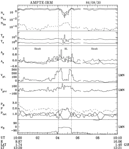
Fig. 4. Overview of the magnetopause
pass on 30 August 1984. The format is the same as in Fig. 1.
3.2 Crossings on 30 August 1984
Figure 4, as well as panels a and b of Fig. 5 present a close pair of magnetopause crossings on 30 August 1984 at 2◦ northern GSM latitude at 12:20 LT. Both crossings can be identified as a sudden change in the angle ϕBby more than
90◦. The inbound crossing occurs at 10:04:05 UT and the outbound crossing at 10:05:23. Between the two crossings, the IRM encounters the boundary layer. For this event, it is not possible to distinguish two separate parts of the boundary layer. While the electron distributions change gradually, the ion distributions are highly variable. Note the rather smooth transition of the total density Ne, and the partial densities
N1e, N2eon the one hand, and the large variation of Tpand
Ap = Tpk/Tp⊥− 1 on the other hand. As we will see, the
high values of Apin the vicinity of the magnetopause are due
to counterstreaming of different ion components.
In the panel of VpL, we recognize, the northward directed
reconnection flows. The existence of a de Hoffmann-Teller frame and the agreement with the Wal´en relation (2) was al-ready tested for these flows by Paschmann et al. (1986) and
Sonnerup et al. (1990). They found a good de Hoffmann-Teller frame and a fairly good correlation of the time series of Vp and cA. For the interval between 10:03:48–10:04:27
around the inbound crossing and for the interval between 10:05:06–10:05:45 around the outbound crossing, the de Hoffmann-Teller frame has CEc,EHT = 0.89, ΛEc,EHT = 0.90 and CEc,EHT = 0.94, ΛEc,EHT = 0.96, respectively.
The cross-correlation CV,cA of the components along the
maximum variance direction of B equals +0.6 and +0.8, re-spectively, indicating Bn < 0. The existence of a normal
magnetic field Bn directed inward is confirmed by the
elec-tron distributions taken in the boundary layer at 10:04:16 and 10:04:46 (Fig. 5a), which show solar wind electrons stream-ing parallel to B, i.e. inward along open field lines. In the magnetosheath (10:02:10 and 10:04:03), the solar wind elec-trons exhibit a reduced flux along the spin axis which is due to an instrumental defect, described in Appendix 1 of Paschmann et al. (1986).
In Fig. 5b, we see a series of ion distributions mea-sured in the magnetosheath well before the inbound cross-ing (10:02:49), in the magnetosheath close to the inbound
a)ELECTRONS,J e (v ) AMPTE-IRM 84/08/30 b)IONS,f p (v ) AMPTE-IRM 84/08/30
Fig. 5. Ion distributions in the energy
range of 20 eV–4 keV and electron dis-tributions in the range of 15 eV–3 keV measured on 30 August 1984. The for-mat is the same as in Fig. 2.
magnetopause crossing (10:03:37), in the dense part of the boundary layer (10:04:25), and finally in its dilute part (10:04:42). The two magnetosheath distributions show an incident solar wind component flowing parallel to B with
Vi0k≈ +0.6cAin the de Hoffmann-Teller frame. Close to the
magnetopause, reflected solar wind ions appear. As expected for reflection at a thin current layer, the field-aligned flow ve-locities in the de Hoffmann-Teller frame of the reflected (Vr0k)
and incident (Vi0k) component fulfill Vr0k = −V
0 ik, V
0 ik > 0
and Vr0k < 0 which is consistent with Bn < 0, as deduced
from the test of the Wal´en relation and the electron distribu-tions in the boundary layer. The appearance of the reflected ions leads to the detected increase in Apafter ∼10:03.
In the boundary layer at 10:04:25, we recognize a maxi-mum of the proton temperature anisotropy, Ap≈ 1.5. As can
be seen in Fig. 5b, this field-aligned anisotropy is also due to counterstreaming of two components: the solar wind ions that have been transmitted across the magnetopausewhich have vk0 > 0, which is again consistent with Bn < 0 and
much colder ions, presumably of ionospheric origin which have v0k < 0 and thus stream outward along open field lines
with Bn < 0. Due to the presence of the ionospheric ions,
the field-aligned bulk velocity Vp0kin the de Hoffmann-Teller
frame is only +0.05cAin the boundary layer. As described
in Paschmann et al. (1985), Vpwas computed under the
as-sumption that all the ions were protons. If the ionospheric component contained many heavy ions, the actual Vp0kmight
even be negative. Although Vp0k/cA is significantly
differ-ent from +1, the reflected ions in the magnetosheath, the
counterstreaming ions in the boundary layer, and the elec-tron distributions in the boundary layer provide evidence for open field lines. At 10:04:42, in the dilute part of the bound-ary layer, no ions are visible within the energy range of Fig. 5b. However, the IRM detects hot ring current ions with
KT ≈ 5 keV at that time.
3.3 Crossing on 17 September 1984
Figure 6 presents an overview of the inbound magnetopause crossing on 17 September 1984, which occurs at the 22◦ southern GSM latitude at 14:10 LT. The magnetopause is crossed at 10:47:58 UT. The rotation of the magnetic field across the magnetopause is low (|∆ϕB| ≈ 15◦) and we can
see a clear plasma depletion layer (Zwan and Wolf, 1976). In Fig. 6, the plasma pressure decreases before 10:47:58 and the magnetic pressure increases. Furthermore, the existence of a plasma depletion layer is reflected in the strong per-pendicular anisotropy, Ap ≈ −0.8, of the proton
tempera-ture in the magnetosheath adjacent to the magnetopause. Per-forming a statistical survey, Phan et al. (1994) found that all low shear crossings have a plasma depletion layer, consistent with the expectation that magnetic reconnection is absent or less efficient between magnetic fields that are nearly paral-lel. The low shear magnetopause crossing on 17 September 1984 was included in their data set and it was also studied by Paschmann et al. (1993). In this section, we will show that the absence of magnetic reconnection, as inferred from the existence of a plasma depletion layer, is confirmed by tests
L
M
Sheath OBL Sphere IBL OBL IBL Sp.
Fig. 6. Overview of the magnetopause
pass on 17 September 1984. The format is the same as in Fig. 1.
for the prediction of a rotational discontinuity which will re-veal that the local magnetopause is closed.
Since |∆ϕB| is small, it is not possible to identify the
mag-netopause with the magnetic field data. But it is clearly visi-ble in the plasma moments (Paschmann et al., 1993). Most striking is the sharp increase in Ap from its low value of
about −0.8 in the plasma depletion layer to values of almost 0 after 10:47:58.
Similar to the high shear crossing on 21 September 1984, three different regions can be distinguished earthward of the magnetopause. From 10:47:58 to ∼10:50:20 and from 10:53:35 to 10:59:09, the IRM encounters the dense plasma of the OBL. Between ∼10:50:20 and ∼10:51:50 and after
∼11:03:30, IRM is located in the magnetosphere proper. An
IBL with properties similar to those of the IBL observed on 21 September 1984 is encountered from ∼10:51:50 to 10:53:35 and from 10:59:09 to ∼11:03:30. In Fig. 6, the difference between the IBL and the magnetosphere is vis-ible in the traces of N1e and Ae = Tek/Te⊥ − 1. It is
not possible to find a de Hoffmann-Teller frame for the in-terval between 10:47:27–10:48:37 around the magnetopause
(CEc,EHT = 0.57, ΛEc,EHT = 1.51). Moreover, the time
series of Vpand cAare not correlated with one another,
con-firming that the local magnetopause is closed.
Figure 7b presents a series of ion distribution functions measured on 17 September 1984 in the magnetosheath (10:47:07), the OBL (10:54:10), the IBL (11:02:01), and the magnetosphere (11:04:55). We recognize that the solar wind population has a strong perpendicular anisotropy in the plasma depletion layer and is more isotropic in the OBL. A few solar wind ions are also detected in the IBL: note the nar-row gray patch at v ≈ 200 km/s in the distribution taken at 11:02:01. Furthermore, hot ring current ions are observed in the IBL and magnetosphere proper. Having KT ≈ 10 keV, they lie outside the energy range selected for Fig. 7b. None of the ion distributions show particle signatures predicted for open field lines.
Figure 7a presents electron distribution functions mea-sured in the four regions. At 10:46:45 in the magnetosheath, the IRM detects solar wind electrons with KT ≈ 30 eV. Across the magnetopause the field-aligned temperature of the solar wind electrons increases by a factor of 2, while their
a)ELECTRONS,J e (v ) AMPTE-IRM 84/08/30 b)IONS,f p (v ) AMPTE-IRM 84/08/30
Fig. 7. Ion distributions in the energy
range of 20 eV–4 keV and electron dis-tributions in the range of 15 eV–3 keV measured on 17 September 1984. The format is the same as in Fig. 2.
perpendicular temperature increases only slightly. Unlike the distribution taken in the OBL on 21 September 1984, the electron distributions observed in the OBL on 17 Septem-ber 1984, e.g. at 10:53:53, do not show any evidence for open magnetic field lines. The distributions taken in the IBL (11:02:23) and magnetosphere proper (11:04:38) are similar to those observed on 21 September 1984. In the magneto-sphere proper, we find cold (KT ∼ 10 eV) electrons pre-sumably of ionospheric origin at velocities v < 4000 km/s and hot (KT ≈ 1 keV) ring current electrons at veloci-ties v > 10 000 km/s. Outside the energy range shown in Fig. 7a, a second ring current component with thermal en-ergy KT ∼ 10 keV is detected. Both ring current compo-nents show the perpendicular temperature anisotropy charac-teristic of particles trapped in the geomagnetic field. In the IBL, e.g. at 11:02:23, we recognize again warm electrons at field-aligned velocities vk≈ 8000 km/s.
Similar to the crossing on 21 September 1984, important information about the IBL, can be deduced from the time se-ries of N2e and VpM. In the IBL the partial density N2e of
electrons above 1.8 keV is again comparable to N2e in the
magnetosphere proper, but it drops in the OBL. Of course, this drop is also visible in Fig. 7a. The trace of VpM
in-dicates again a flow reversal at the interface between the OBL and the IBL. Since the IRM is located at 14:00 LT, the magnetosheath flow has a duskward component, VpM ≈
−100 km/s. While the flow in the OBL shares this duskward
motion, the flow in the IBL and magnetosphere proper is di-rected dawnward. This reveals that the plasma in the IBL is
not magnetically or viscously coupled to the magnetosheath plasma. Rather, the dawnward motion is consistent with the return flow of a closed magnetic flux from the nightside back to the dayside.
While the time series of N2e and VpM provide evidence
that the IBL is on closed field lines, it is difficult to decide on the state of the OBL. On the one hand, the existence of a plasma depletion layer and tests for the prediction of a ro-tational discontinuity imply that the magnetopause is locally closed. On the other hand, cross-field diffusion should not be able to form an OBL whose density and temperature pro-files show a plateau (10:53:35–10:59:09) with a sharp step at its inner edge. A possible explanation for the OBL on 17 September 1984 would be that it is on open field lines that cross the magnetopause at a location farther away from the spacecraft. In this case, the solar wind plasma detected in the OBL may have entered along open field lines. If these field lines do not cross the magnetopause locally but farther away from the spacecraft, there is no reason why the observed lo-cal magnetopause should have the properties of a rotational discontinuity.
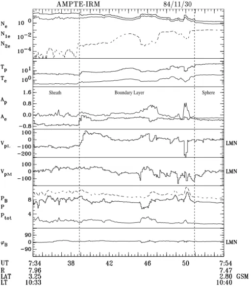
3.4 Crossing on 84/11/30
Figure 8 presents an overview of the inbound magnetopause crossing on 30 November 1984, which occurs at the 3◦ northern GSM latitude at 10:30 LT. We identify the magne-topause as the increase in the proton temperature, the elec-tron temperature, and the temperature anisotropies, Ap and
L
M
Sheath Boundary Layer Sphere
Fig. 8. Overview of the magnetopause
pass on 30 November 1984. The format is the same as in Fig. 1.
Ae, at 07:38:51. The panel of ϕB shows that the direction
of the tangential magnetic field does not change across the magnetopause. Immediately earthward of the magnetopause the component VpL of the proton bulk velocity changes by
about 200 km/s. Since this change of the tangential veloc-ity is not accompanied by any change of the tangential mag-netic field, the Wal´en relation (2) cannot be satisfied. Since in the interval 07:37:52–07:39:50 around the magnetopause
CEc,EHT = 0.59, ΛEc,EHT = 2.86, we conclude that a de
Hoffmann-Teller frame is improbable during this interval at least when it is based on our analysis.
The boundary layer lasts from 07:38:51 to ∼07:50:55. During this interval, the density oscillates a few times be-tween about 20 cm−3and 2 cm−3. The temperatures Tpand
Teexhibit similar oscillations. Since the temporal profiles of
these oscillations are gradual rather than in steps, we do not distinguish between the OBL and the IBL.
Panel a of Fig. 9 presents a series of electron distribu-tions measured on 30 November 1984 in the magnetosheath (07:38:20), the magnetosheath closer to the magnetopause (07:38:42), the boundary layer (07:40:05), and the
magneto-sphere proper (07:52:38). Panel b shows the ion distribution functions measured at the same times. In the magnetosphere, the IRM detects hot ring current ions with KT ≈ 6 keV and ring current electrons with KT ≈ 0.5 keV. Both species show the perpendicular temperature anisotropy of trapped particles.
The electron distribution taken at 07:38:20 in the mag-netosheath shows solar wind electrons with thermal energy
KT ≈ 30 eV. Closer to the magnetopause (07:38:42), the
electron distribution becomes skewed along the magnetic field: it remains unchanged for vk < 0, whereas the other
half of the distribution (vk > 0) is much flatter than at
07:38:20 and thus extends to higher energies. Skewed dis-tributions such as the one taken at 07:38:42 were already re-ported by Fuselier et al. (1995) and interpreted as a feature of the magnetosheath boundary layer, i.e. the portion of the magnetosheath on reconnected field lines. According to this model, the electron distribution at 07:38:42 would indicate magnetic connection to the southern hemisphere (Bn > 0).
Since Bn > 0 electrons with vk < 0 come from the
distribu-a)ELECTRONS,J e (v ) AMPTE-IRM 84/11/30 b)IONS,f p (v ) AMPTE-IRM 84/11/30
Fig. 9. Ion distributions in the energy
range of 20 eV–4 keV and electron dis-tributions in the range of 15 eV–3 keV measured on 30 November 1984. The format is the same as in Fig. 2.
tion antiparallel to B looks the same in the magnetosheath boundary layer as wellas in the magnetosheath on interplan-etary field lines which are not yet reconnected. Electrons in the magnetosheath boundary layer with vk > 0 come from
the terrestrial end of an open field line; the half of the dis-tribution parallel to B should look similar to the low-latitude boundary layer earthward of the magnetopause. The electron plasma observed in the boundary layer at 07:40:05 has in-deed a higher temperature than that in the magnetosheath, which could explain why the half of the distribution parallel to B at 07:38:42 is flatter than the half of the distribution an-tiparallel to B. In the model of Fuselier et al. (1995), solar wind electrons are heated when they cross the open mag-netopause antiparallel to B from the magnetosheath to the boundary layer. After mirroring at low altitudes, they cross the open magnetopause again from the boundary layer to the magnetosheath and can be observed in the magnetosheath boundary layer, now moving parallel to B. The reason for the electron heating across the magnetopause is not known, but it is well established by observations (e.g. Paschmann et al., 1993) that the solar wind population in the boundary layer is primarily hotter than in the magnetosheath (see also Fig. 7a). The half of the distribution parallel to B at 07:38:42 is even flatter than the distribution in the low-latitude boundary layer. One might speculate that this is the case due to the outward moving electrons in the magnetosheath boundary layer cross-ing the magnetopause twice and, therefore, heatcross-ing twice. The heating of solar wind electrons is of course only one rea-son for the increase in Teacross the magnetopause. The other
reason is the admixture of hot ring current electrons. For
v > 20 000 km/s, the phase space density in the
magneto-sphere proper is clearly higher than in the boundary layer and magnetosheath. Therefore, electrons with v > 20 000 km/s at 07:38:42 are probably ring current electrons leaking out to the magnetosheath.
Let us return to the ion distributions. At 07:38:20 and 07:38:42, the IRM detects the solar wind population of the magnetosheath. At 07:40:05 in the boundary layer, we see two components, i.e. two peaks of fp(v). One component
appears at the same position in velocity space as the solar wind population in the magnetosheath. Thus, this compo-nent probably consists of solar wind ions that have entered the boundary layer locally due to diffusion or reconnection. The second component has a high field-aligned flow veloc-ity, Vk ≈ 350 km/s, which suggests that it has entered the
boundary layer at a location south of the spacecraft. At that location, either the flow velocity in the magnetosheath was different from the flow velocity observed in the local mag-netosheath, or the acceleration across the magnetopause was different. The appearance of this second component is re-sponsible for the change in VpL around 07:39. Both
com-ponents are observed throughout the boundary layer. There are several many IRM magnetopause passes that show ion distributions in the boundary layer with two solar wind com-ponents.
at least one particle signature 75% 38% bipolar Bnsignature 46% 0%
4 Data set for statistical survey
We studied all IRM passes through the dayside (08:00–16:00 LT) magnetopause region for which magnetometer measure-ments, plasma moments at spin resolution, ion and electron distribution functions of the full energy-per-charge range, and electric wave spectra are available. The statistical data set, analyzed in this paper and in paper 2, contains all magne-topause crossings that occurred during these passes and that fulfill the following selection criteria: (1) The crossing is a complete crossing from the magnetosheath to the magneto-sphere proper (or vice versa). (2) The boundary layer lasts for ∆tBL> 30 s. (3) At least two electron distribution
func-tions are measured in the boundary layer. (4) The time inter-vals in the magnetosheath before (after) the boundary layer and the time interval in the magnetosphere after (before) the boundary layer are sufficiently long so that an unambiguous identification of the magnetopause and of the earthward edge of the boundary layer is possible.
Criteria 2 and 3 are required in order to resolve the inter-nal structure of the boundary layer, i.e. to distinguish grad-ual time profiles from step like profiles. Due to criterion 2, our data set is likely to be biased toward crossings of thick boundary layers. Note, however, that Phan and Paschmann (1996) found a trend for crossings with long boundary layer duration to result from lower magnetopause speeds. Thus boundary layers lasting more than 30 s need not necessarily be much thicker than those of a shorter time duration.
With the above selection criteria, we obtained 40 mag-netopause crossings. The magmag-netopause crossings on 17 September 1984 (Sect. 3.3), on 21 September 1984 (Sect. 3.1), and on 30 November 1984 (Sect. 3.4) are in-cluded in the statistical data set. However, the two crossings on 30 November 1984 (Sect. 3.2) are not included, since the IRM does not encounter the magnetosphere proper.
We will distinguish between low and high magnetic shear. Choosing 40◦ as the dividing line, we obtain 16 low shear (|∆ϕB| < 40◦) crossings and 24 high shear (|∆ϕB| > 40◦)
crossings. All crossings occurred near the equatorial plane, at latitudes less than 30◦. The numbers of crossings in the local time sectors 08:00–10:00, 10:00–12:00, 12:00–14:00, and 14:00–16:00 are 12, 14, 7, and 7, respectively.
centered at the magnetopause that is at least 20 s long, but may be much longer if the duration of the boundary layer is long.
First, an estimate of the de Hoffmann-Teller velocity,
VHT, is determined by minimizing the quadratic form D of
Eq. (1). For a reasonable de Hoffmann-Teller frame, we re-quire that the minimum of D is well-defined and that VHT
is stable when the interval used for the test is varied. Then the fit between Ec = −Vp× B and EHT = −VHT× B
is checked by producing a single scatter plot of −Vp× B
versus −VHT× B (Sonnerup et al., 1987, 1990; Paschmann
et al., 1990) and its correlation coefficient and linear regres-sion coefficients are calculated. Moreover, we calculate the cross correlation and the linear regression coefficients of the time series of the components −Vp × B and −VHT× B
along the maximum variance direction of −Vp× B.
Inspect-ing the scatter plots and the correlation and regression coef-ficients, we find that 26 of the 40 crossings have a reasonable de Hoffmann-Teller frame. For 10 of the 14 events without de Hoffmann-Teller frame, the magnetic shear across the mag-netopause is low (|∆ϕB| < 40◦) and for 4 events, it is high
(|∆ϕB| > 40◦).
The agreement with the Wal´en relation (2) is checked with the help of the scatter plot of Vp0 = Vp− VHT versus cA
and by calculating the correlation and linear regression co-efficients. We also calculate the cross correlation and linear regression coefficients of the time series of the components
V0pand cAalong the maximum variance direction of B. We
find that 13 of the 26 magnetopause crossings have a reason-able de Hoffmann-Teller frame and the relation
V0p= ΛcA (3)
is approximately satisfied. For the remaining 13 crossings.
V0pand cAare not correlated .
One of the 13 magnetopause crossings satisfying Eq. (3) agrees perfectly with the Wal´en relation (|Λ| = 1). For 2 crossings, |Λ| is only 0.2. For the remaining 10 crossings,
|Λ| is in the range of 0.4–0.8. The fit between the
predic-tion of the Wal´en relapredic-tion and the measured plasma moments and magnetic fields was tested in numerous studies of mag-netopause crossings (e.g. Paschmann et al., 1986, 1990; Son-nerup et al., 1987, 1990). As in our survey, it was found that a linear relation (3) existed for many crossings, but the mag-nitude of the slope Λ is primarily less than 1.
What can we infer from the linear relation (3)? First, Eq. (3) gives a qualitative indication of an open magne-topause. There is no reason to expect such a relation for a closed magnetopause. On the other hand, a magnetopause crossing that satisfies Eq. (3) with |Λ| < 1 does not agree quantitatively with the theory of the rotational discontinu-ity. We have noted reasons for the deviations in the
Intro-duction (see also Scudder, 1997). It cannot be expected that our analysis which is based on ion bulk flows will provide ideal agreement. But the existence of a satisfactory fit to the above equation can safely be taken as confirmation of an approximate validity of the model. The three magnetopause crossings studied in Sects. 3.1 and 3.2 provided us with ad-ditional information concerning the interpretation of Eq. (3). Although |Λ| is significantly less than 1 for those crossings, the observed particle signatures in the distribution functions provide some evidence for open field lines. The sign of Bn
inferred from the particle signatures is consistent with the sign of Bninferred from Eq. (3).
In Sect. 7, we will investigate how often particle signatures expected on open field lines occur during the 40 crossings of the statistical data set. For particle signatures observed during the 13 magnetopause crossings showing a linear relation (3), the sign of Bnas inferred from the respective particle
signa-ture will be compared with the sign of Bn as inferred from
Eq. (3). As we will see, there are observations of particle sig-natures for which the sign of Bn inferred from the particle
signature differs from the sign of Bn inferred from Eq. (3).
But for the clear majority of observations of particle signa-tures, the sign of Bninferred from the particle signature
coin-cides with the sign of Bninferred from Eq. (3). For the types
of particle signatures observed frequently, this coincidence shows that it is correct, in a statistical sense, to interpret the respective type of particle signature in terms of open field lines. Vice versa, it can also be concluded that it is correct, in a statistical sense, to consider the validity of Eq. (3) as an in-dication of an open magnetopause. Hence, we will from now on consider the validity of Eq. (3) as a “reasonable agree-ment with the Wal´en relation” and refer to the magnetopause crossings showing a linear relation (3) as “Wal´en events”. The reasons why |Λ| is, in general, less than 1 will be dis-cussed in Sect. 8.
For 9 of the 13 Wal´en events, the sign of Λ is positive, which indicates Bn < 0 and for 4 events it is negative
(Bn > 0). For 11 of the 13 Wal´en events, the boundary
layer can be divided into an OBL and IBL, whereas 2 Wal´en events have a gradual density profile. Three of the 13 Wal´en events are low shear crossings and 10 are high shear cross-ings. The percentage of Wal´en events and non-Wal´en events for high and low magnetic shear across the magnetopause, respectively, is illustrated in Table 1.
In their survey of a set of IRM high shear crossings, Phan et al. (1996) checked the fit between the observed change
∆Vp of the proton bulk velocity across the magnetopause
and the change ±∆cAof the Alfv´en velocity. ∆Vpand ∆cA
were both computed for each measurement in the boundary layer as the difference between the respective measurement in the boundary layer and the average of a reference interval in the magnetosheath. For each magnetopause crossing, the agreement with the prediction of Eq. (2) was then quantified by computing the index
∆V∗=∆Vp· ∆cA |∆cA|2
(4)
Finally, a magnetopause crossing was considered to be in rea-sonable agreement with the Wal´en relation, if |∆V∗|
evalu-ated at the time of the maximum observed velocity change
∆Vpwas greater than 0.5. Using this criterion, which differs
from ours, Phan et al. (1996) found that 61% of the high shear crossings are in reasonable agreement with the Wal´en rela-tion, whereas our survey reveals that 42% of the high shear crossings are Wal´en events.
6 Flux transfer events
By looking for clear bipolar pulses in the time series of the normal magnetic field, Bn, we can identify magnetosheath
FTEs during 5 of the 40 magnetopause crossings and mag-netospheric FTEs during 9 of the 40 magnetopause crossings in our data set. During 3 crossings, both magnetosheath and magnetospheric FTEs are observed and during 8 crossings, only one type of FTEs is observed. For 3 of the 11 cross-ings with FTEs, the magnetic shear angle, |∆ϕB|, measured
across the magnetopause is 50◦–60◦. The remaining 8 cross-ings had shear angles of 90◦or more. This is in line with the finding (e.g. Rijnbeek et al., 1984; Southwood et al., 1986) that FTEs are favored by a southward directed interplanetary magnetic field.
In the original FTE model of Russell and Elphic (1978), an FTE is an encounter with a reconnected magnetic flux tube. A flux tube moving northward causes a +− bipolar signa-ture of Bn, whereas a flux tube moving southward causes a
−+ signature. If the motion of the flux tube is dominated
by the magnetic tension force, a flux tube connected to the northern hemisphere (Bn< 0) moves northward and causes
a +− signature, whereas a flux tube connected to the south-ern hemisphere (Bn> 0) moves southward and causes a −+
signature. Assuming that the motion of the flux tube is dom-inated by the tension force, one can thus infer the sign of the normal magnetic field Bnin the reconnected flux tube from
the orientation (+− or −+) of the bipolar signature. For the Wal´en events in our data set, we can compare the sign of Bninferred from the bipolar signature of FTEs with
the sign of Bnas inferred from Eq. (3). Magnetosheath FTEs
are observed during 3 of the 13 Wal´en events and magneto-spheric FTEs are observed during 5 of the 13 Wal´en events. We find that for all FTEs observed during Wal´en events, the sign of Bninferred from the bipolar signature coincides with
the sign of Bn inferred from Eq. (3). Thus, we can explain
all FTEs observed during Wal´en events as encounters with reconnected flux tubes that are connected to the same hemi-sphere as the field lines in the vicinity of the magnetopause and that move toward the hemisphere to which they are con-nected. Our result can also be explained by other reconnec-tion models of FTEs. In any case, it provides evidence for FTEs as a signature of magnetic merging.
electron heat flux 62% (54%) 15% escaping RC ions 31% (31%) 0%
D-shaped 23% (23%) 15%
counterstr. SW/cold 23% (15%) 19% skewed SW distr. 62% (54%) 15% at least one part. sign. 77% 52% bipolar Bnsignature 62% (62%) 19%
7 Occurrence of particle signatures
In Sect. 3 we reported on examples of observations of several types of single particle signatures expected on open magnetic field lines. Now we study the occurrence frequency of the various types of particle signatures. For Wal´en events, we compare the sign of Bnas inferred from the respective
parti-cle signature with the sign of Bninferred from Eq. (3). If the
number of Wal´en events, for which a particular type of par-ticle signature is consistent with Eq. (3), is high compared to the number of Wal´en events for which it is not consistent, the respective type of signature can be considered as a reliable indicator of open field lines. If these two numbers are compa-rable, the respective signature may be caused by mechanisms other than reconnection. In Table 2 the occurrence rates are given as percentages.
7.1 Electron heat flux
In Sect. 3 we examined two kinds of electron distributions as-sociated with substantial heat flux along the magnetic field. On 21 September 1984 at 13:01:05 (Fig. 2a), the heat flux is caused by hot ring current electrons escaping along B from the magnetosphere to the magnetosheath. On 30 November 1984 at 07:38:42 (Fig. 9a), part of the heat flux is due to a skewed distribution of solar wind electrons. Both the escape of ring current electrons and the skewed distribution of so-lar wind electrons (Fuselier et al., 1995) are expected to lead to heat flux that is directed outward from the magnetosphere to the magnetosheath. Thus, heat flux antiparallel to B indi-cates Bn < 0 and heat flux parallel to B indicates Bn > 0.
How often do we observe substantial electron heat flux at the magnetopause?
In Sects. 7.1 to 7.5 we study the occurrence frequency of various types of particle signatures by counting the magne-topause crossings in the data set during which the respective type of signature is observed. When we count the crossings, we take only crossings for which the particular type of par-ticle signature fulfills the following criteria: (1) The parpar-ticle signature is clearly visible when the measured distribution functions are inspected by eye. (2) The orientation of the
par-bution within a spin period of IRM. Furthermore, criterion 2 sorts out magnetopause crossings for which the electron heat flux is strong, but changes its orientation in the course of the crossing from parallel to B to antiparallel to B or vice versa. Such observations might indicate time dependent patchy re-connection or encounters with the vicinity of the X-line. However, they cannot be used to infer the sign of Bn from
the orientation of the electron heat flux or to check whether this sign is consistent with Eq. (3). The implications of crite-ria 1 and 2 for the other particle signatures of Sects. 7.2 to 7.5 are analogous.
Applying criteria 1 and 2, we count the magnetopause crossings with electron heat flux. Thereby, we do not dis-tinguish whether the heat flux is due to a streaming of ring current electrons or due to a field-aligned, skewed distribu-tion of solar wind electrons. We find that electron heat flux is observed during 12 of the 40 magnetopause crossings in the data set. Of those 12 crossings, 8 are Wal´en events. For one Wal´en event the orientation of the electron heat flux is inconsistent with the sign of Bn inferred from Eq. (3), but
it is consistent for the other 7 Wal´en events. Hence, electron heat flux fulfilling criteria 1 and 2 is primarily consistent with Eq. (3) and can, in a statistical sense, be considered as a use-ful indicator of open field lines.
7.2 Escape of ring current ions
On 21 September 1984 at 13:01:39 (Fig. 3), we observe hot ring current ions escaping from the magnetosphere to the magnetosheath. This escape along open field lines is asso-ciated with a substantial outward directed proton heat flux,
Hpk ≈ −0.05 mW/m2. Inspecting all ion distribution
func-tions measured during the crossings of the statistical data set, we find a streaming of ring current ions for 4 out of the 40 crossings. These 4 magnetopause crossings are all Wal´en events and the orientation of the outward directed heat flux is consistent with the sign of Bninferred from Eq. (3).
7.3 “D-shaped” distributions of solar wind particles On 21 September 1984 at 13:01:05 (Fig. 2), we observe “D-shaped” distributions of solar wind ions and electrons. When we search for “D-shaped” distributions of solar wind parti-cles in the statistical data set, we require that the measured phase space density is cut off at vk0 ≈ 0, as observed on 21
September 1984 at 13:01:05. We find that “D-shaped” distri-butions of solar wind electrons are measured during 2 of the 40 crossings. On 21 September 1984 the orientation of the “D” is consistent with the sign of Bninferred from Eq. (3).
The other crossing is not a Wal´en event. “D-shaped” distri-butions of solar wind ions are measured during 5 of the 40
crossings. For all 5 crossings, the magnetic shear across the magnetopause is high. Of the 5 crossings, 2 are Wal´en events and for these 2 crossings, the orientation of the “D” is con-sistent with the sign of Bninferred from Eq. (3).
7.4 Counterstreaming of solar wind ions and cold ions On 30 August 1984 at 10:04:25 (Fig. 5b), we observe so-lar wind ions streaming inward along open field lines and cold ions, presumably of ionospheric origin, simultaneously streaming outward. By looking for the counterstreaming of solar wind and cold ions in the entire data set, we find this signature for 8 out of 40 crossings. Three of these 8 crossings are Wal´en events. If the counterstreaming is due to magnetic reconnection, it can be used to infer the sign of the normal magnetic field Bn: streaming of the solar wind ions relative
to the cold ions parallel (antiparallel) to B indicates Bn< 0
(Bn > 0). For 2 of the 3 Wal´en events, the sign of Bn
in-ferred from the counterstreaming agrees with the sign of Bn
inferred from Eq. (3).
The crossing where the counterstreaming of solar wind and cold ions is inconsistent with Eq. (3) occurred on 30 Au-gust 1984 at 09:56:43, roughly 8 min before the two cross-ings studied in Sect. 3.2. Remember that those two crosscross-ings are not included in our data set, because the magnetosphere proper is not encountered. Similar to the other two crossings, the test of the Wal´en relation indicates Bn < 0 for the
mag-netopause crossing at 09:56:43. Immediately earthward of the magnetopause, the flow velocity of the transmitted solar wind component in the de Hoffmann-Teller frame is about 200 km/s. At 09:51:54, when the counterstreaming of solar wind and cold ions is observed, the flow velocity of the solar wind component in the de Hoffmann-Teller frame is about
−500 km/s. Thus, the solar wind component at 09:51:54
cannot be identical to the transmitted component observed immediately earthward of the magnetopause. The field lines encountered at 09:51:54 are probably topologically different from those encountered immediately earthward of the mag-netopause.
7.5 Skewed distributions of solar wind ions
What do we mean by skewed distributions? Two examples of skewed distributions of solar wind ions are those measured on 30 August 1984 at 10:03:37 (Fig. 5b) and on 30 Novem-ber 1984 at 07:40:05 (Fig. 9b). Both distributions show two beams, i.e. two peaks of fp(v). The reflected solar wind
ions detected on 30 August 1984 at 10:03:37 in the mag-netosheath close to the magnetopause lead to a field-aligned heat flux, Hpk ≈ −0.14 mW/m2. In the magnetosheath we
furthermore observe ion distribution functions that are also associated with a substantial field-aligned heat flux, but do not show two peaks of fp(v). Rather these distributions
con-sist of a steep, half parallel to B, and a flat, half antiparallel to B or vice versa. By examining both of these “steep-flat” distributions and the two-beam distributions observed in the magnetosheath for Wal´en events, we find that the proton heat
flux associated with these distributions is, in most cases, out-ward along open field lines.
“Steep-flat” distributions are also observed in the bound-ary layer, the heat flux associated with “steep-flat” distri-butions measured during Wal´en events is directed outward along open field lines in most cases, as well. The distribu-tion taken on 30 Nobember 1984 at 07:40:05 is an exam-ple of a two-beam distribution measured in the boundary layer. It is associated with a substantial proton heat flux,
Hpk ≈ 0.08 mW/m
2.
Why do we observe two beams in the boundary layer? One possibility is that beam 1 consists of locally entering ions and beam 2 consists of ions that have entered the boundary layer at a remote location. This interpretation was given for the dis-tribution measured on 30 November 1984 at 07:40:05. Simi-lar two-beam distributions have been presented by Nakamura et al. (1997). Another possibility is that beam 2 is produced when beam 1 is mirrored at low altitudes. In this case, the field-aligned components of the flow velocities of the two beams should have about the same magnitude, but opposite sign in the spacecraft frame. Two-beam distributions fulfill-ing this condition were reported by Onsager and Fuselier (1994) and are also seen in the IRM data.
Can we use skewed distributions of solar wind ions to in-fer the sign of the normal magnetic field Bn? In the
follow-ing, we try to infer Bn for three types of skewed
distribu-tions: (1) If we observe distributions of solar wind ions in the magnetosheath associated with a field-aligned heat flux, we assume that the heat flux is directed outward. (2) If we observe “steep-flat” distributions in the boundary layer, we assume that the heat flux is directed outward. (3) If we ob-serve two-beam distributions in the boundary layer and are able to identify beam 1 as the component of locally entering solar wind ions, we assume that the field-aligned velocity of beam 2 relative to beam 1 is directed outward.
We find distribution functions of types 1–3 for 12 of the 40 magnetopause crossings in the data set. Eight of these 12 crossings are Wal´en events. By comparing the sign of Bn
in-ferred from Eq. (3) with the sign of Bn inferred from the
skewed distributions with the above assumptions, we find that those two methods of inferring the sign of Bn lead to
the same result for 7 of the 8 Wal´en events. Hence, skewed distributions of solar wind ions can, in a statistical sense, be considered as a useful indicator of open field lines.
7.6 Events with at least one type of signature
So far, we counted the number of crossings showing a par-ticular type of particle signature. Let us, in addition, count the number of magnetopause crossings that show at least one of the types of particle signatures studied in Sects. 7.1 to 7.5. We find that the particle signatures are more frequent for high shear (18 out of 24 crossings) than for low shear (6 out of 16). During 10 of the 13 Wal´en events, at least one particle signature of open field lines is observed. The corresponding percentages are given in Tables 1 and 2.