HAL Id: hal-00077722
https://hal.archives-ouvertes.fr/hal-00077722
Submitted on 15 Nov 2020
HAL is a multi-disciplinary open access
archive for the deposit and dissemination of
sci-entific research documents, whether they are
pub-lished or not. The documents may come from
teaching and research institutions in France or
abroad, or from public or private research centers.
L’archive ouverte pluridisciplinaire HAL, est
destinée au dépôt et à la diffusion de documents
scientifiques de niveau recherche, publiés ou non,
émanant des établissements d’enseignement et de
recherche français ou étrangers, des laboratoires
publics ou privés.
Ozone Hole on the Midlatitudes
Marion Marchand, Slimane Bekki, Andrea Pazmino, Franck Lefèvre, Sophie
Godin-Beekmann, Alain Hauchecorne
To cite this version:
Marion Marchand, Slimane Bekki, Andrea Pazmino, Franck Lefèvre, Sophie Godin-Beekmann, et al..
Model Simulations of the Impact of the 2002 Antarctic Ozone Hole on the Midlatitudes. Journal of the
Atmospheric Sciences, American Meteorological Society, 2005, 62, pp.871-884. �10.1175/JAS-3326.1�.
�hal-00077722�
Model Simulations of the Impact of the 2002 Antarctic Ozone Hole on
the Midlatitudes
M. MARCHAND ANDS. BEKKI
Service d’Aéronomie/IPSL, CNRS, Paris, France
A. PAZMINO
Service d’Aéronomie/IPSL, CNRS, Paris, France, and CEILAP/CITEFA-CONICET, Buenos Aires, Argentina
F. LEFÈVRE, S. GODIN-BEEKMANN,ANDA. HAUCHECORNE
Service d’Aéronomie/IPSL, CNRS, Paris, France
(Manuscript received 11 December 2003, in final form 25 February 2004) ABSTRACT
The 2002 Antarctic winter was characterized by unusually strong wave activity. The frequency and intensity of the anomalies increased in August and early September with a series of minor stratospheric warmings and culminated in a major stratospheric warming in late September. A three-dimensional high-resolution chemical transport model is used to estimate the effect of the exceptional 2002 Antarctic winter on chemical ozone loss in the midlatitudes and in polar regions. An ozone budget analysis is performed using a range of geographical and chemical ozone tracers. To highlight the unusual behavior of the 2002 winter, the same analysis is performed for the more typical 2001 winter. The ability of the model to reproduce the evolution of polar and midlatitude ozone during these two contrasted winters is first evalu-ated against ozonesonde measurements at middle and high latitudes. The evolution of the model-calculevalu-ated 2002 ozone loss within the deep vortex core is found to be somewhat similar to that seen in the 2001 simulation until November, which is consistent with a lower-stratospheric vortex core remaining more or less isolated even during the major warming. However, the simulations suggest that the wave activity anomalies in 2002 enhanced mixing well before the major warming within the usually weakly mixed vortex edge region and, to a lesser extent, within the surrounding extravortex region. As a result of the increased permeability of the vortex edge, the export of chemically activated vortex air is more efficient during the winter in 2002 than in 2001. This has a very noticeable impact on the model-calculated midlatitude ozone loss, with destruction rates being about 2 times higher during August and September in 2002 compared to 2001. If the meteorological conditions of 2002 were to become more prevalent in the future, Antarctic polar ozone depletion would certainly be reduced, especially in the vortex edge region. However, it is also likely that polar chemical activation would affect midlatitude ozone earlier in the winter.
1. Introduction
Since global monitoring of the Southern Hemisphere (SH) winter polar stratosphere, the springtime ozone hole formation has somewhat followed the same pat-tern with a relatively small amount of interannual vari-ability compared to the Northern Hemisphere winter polar stratosphere. The wave activity is usually weak in the Southern Hemisphere. As a result, the Antarctic polar vortex is strong, stable, and rather circular. It is accompanied with very low temperatures and severe
polar ozone destruction in the spring. The polar ozone losses have been increasing more or less steadily for the last two decades (Bodeker et al. 2002). The main pro-cesses involved appear to be relatively well understood [World Meteorological Organization (WMO) 2002]. The low temperatures during the winter lead to the formation of polar stratospheric clouds (PSCs) on which ozone destroying halogen radicals are activated. With the return of sunlight in spring, polar ozone is very rapidly destroyed in the lower stratosphere through chemical cycles catalyzed by halogen radicals. The 2002 Antarctic winter was the exception to the overall pat-tern and trend. That winter was marked by unusually strong planetary wave activity from May onward (Allen et al. 2003), resulting in a rather disturbed Antarctic polar vortex. Three minor warmings during August and early September preceded a major stratospheric
warm-Corresponding author address: Dr. M. Marchand, Service
d’Aéronomie/IPSL, Université Pierre et Marie Curie, B. 102, 4 Place Jussieu, 75230 Paris, Cedex 05, France.
E-mail: [email protected]
© 2005 American Meteorological Society
JAS3326
ing in late September. Total Ozone Mapping Spectrom-eter (TOMS) and Global Ozone Monitoring Experi-ment (GOME) data show that the major warming caused the vortex to apparently split into two parts on 25 September (Varotsos 2002; Sinnhuber et al. 2003). This had never been observed before in the Southern Hemisphere. Height-resolved ozone measurements from the Polar Ozone and Aerosol Measurement III (POAM III) instrument and from Solar Backscattered Ultraviolet (SBUV /2) and Television Infrared Obser-vation Satellite (TIROS-N) Operational Vertical Sounder (TOVS) show that the lower part of the vortex remained more or less intact during the major warming while the middle part split into two distinct lobes (Hop-pel et al. 2003; Kondragunta et al. 2005). One lobe rap-idly mixed with the extravortex air, while the other returned to the Pole as a much weaker and smaller vortex (Allen et al. 2003). Since winter polar chemistry is closely linked to the dynamics of the vortex, the anomalous meteorological conditions of 2002 should have had a pronounced impact on the chemical ozone destruction within and around the vortex. In particular, the very large lobe of the polar vortex that broke away and mixed with extravortex air impacted ozone levels in the midlatitudes in late September. Indeed, polar vor-tex air had already experienced severe ozone destruc-tion and hence was depleted in ozone with respect to midlatitude air. The presence of ozone-depleted air of polar origin was detected in the Stratospheric Aerosol and Gas Experiment III (SAGE III) measurements during the same period (Randall et al. 2005). At the same time, the 2002 warming was accompanied by rapid large-scale transport of air from the extravortex region to the pole bringing ozone-rich air to high lati-tudes, as recorded by the POAM III instrument (Ran-dall et al. 2005).
It has not yet been established whether the excep-tional Antarctic winter of 2002 is indicative of a long-term trend or simply part of the natural variability. Ozone observations of the recent Antarctic winter of 2003 indicate a return to an Antarctic ozone hole more typical of the last two decades with a stable, cold, and large vortex characterized with severe ozone depletion. Nonetheless, it is important to understand the implica-tions of such an anomalous winter for midlatitude ozone, especially if these exceptional meteorological conditions become more prevalent in the future. The importance of the transport of polar air to the midlati-tudes and its impact on midlatitude ozone loss has al-ready been pointed out in a number of studies (Prather and Jaffe 1990; WMO 1994, and references therein). Two commonly associated mechanisms are the trans-port of ozone-depleted polar air into the midlatitudes and of chemically activated polar air followed by in situ ozone destruction. In this paper, we use a high-resolu-tion chemistry transport model to investigate the effect of the exceptional 2002 Antarctic winter on the ozone budget in the midlatitudes. The budget analysis is
per-formed with a chemistry transport model (CTM) con-taining a range of geographical and chemical tracers. Particular attention is paid to accurately estimating the respective contributions of in situ (i.e., midlatitude) chemistry and polar vortex processes to the extravortex ozone loss. To highlight the unusual behavior in 2002, CTM calculations are also performed for the more typi-cal 2001 winter. If these two contrasted meteorologies represent two expected regimes, then the simulations give a vision of expected differences in the future. In the second section, a brief description of the high-resol-ution CTM and the methodology is provided. Section 3 presents an evaluation of the ability of the model to simulate ozone chemistry in the polar and midlatitude regions for the 2001 and 2002 winters. The origins of the model-calculated vortex and extravortex ozone loss in the two winters are diagnosed and contrasted in section 4. The final section is devoted to a summary of the results and conclusions.
2. Description of the model and numerical experiments
a. High-resolution chemistry transport model We use a high-resolution chemistry transport model Mode´le Isentropique de transport Mesoechelle de l’Ozone Stratosphe´rique par Advection avec Chimie (MIMOSA-CHIM), which is described in detail by Marchand et al. (2003). The offline model couples the advection scheme of MIMOSA (Hauchecorne et al. 2002) and the chemical scheme of the Reactive Pro-cesses Ruling the Ozone Budget in the Stratosphere (REPROBUS) model (Lefèvre et al. 1994). The model horizontal resolution is set high (1° latitude⫻ 1° lon-gitude) in order to simulate as accurately as possible the exchanges between the polar vortex and the midlati-tudes. Horizontal winds and temperatures are specified using daily European Centre for Medium-Range Weather Forecasts (ECMWF) 2.5°⫻ 2.5° analyses in-terpolated linearly onto the finer MIMOSA-CHIM horizontal grid. Sixteen isentropic levels are considered covering the 335–1650-K altitude range with a higher vertical resolution in the lower stratosphere where most of ozone destruction usually occurs. The model covers the South Hemisphere down to 30°S. The advection scheme is semi-Lagrangian. To minimize the numerical diffusion, the interpolation associated with the regrid-ding is based on the preservation of the second-order moment of a potential vorticity (PV) perturbation (Hauchecorne et al. 2002). The model run at high reso-lution is able to maintain sharp gradients and reproduce filamentary structures. Vertical advection is derived from heating rates provided by the MIDRAD radiative scheme (Shine 1987; Chipperfield 1999). Heating rates are calculated from global meteorological analysis and climatologies of ozone and water vapor. Heating rates on each global isentropic surface are subsequently cor-rected in order to ensure that the total mass flux
through each isentropic level is null. The model con-tains a PV tracer, which is advected like any other tracer but is relaxed toward ECMWF PV values with a relaxation time of 10 days in order to account for its diabatic evolution (Hauchecorne et al. 2002). The chemical scheme contains a detailed treatment of the stratospheric chemistry of the Ox, NOy, Cly, Bry, and
HOxfamilies (Lefèvre et al. 1994). The model also
in-cludes long-lived tracers such as N2O, CH4, and H2O.
There is a representation of the heterogeneous chem-istry associated with liquid supercooled sulfuric acid aerosols, nitric acid trihydrate (NAT), and ice particles, which are assumed to be in equilibrium with the gas phase (Lefèvre et al. 1998). The denitrification origi-nating from the sedimentation of large NAT particles is also taken into account. An ozone-like passive tracer is also included in the model in order to monitor the ozone changes of chemical origin. This tracer is initialized in the same way as the chemically active ozone at the beginning of the integration and then is advected pas-sively. The model is initialized by linearly interpolating PV fields from ECMWF analyses and REPROBUS chemical fields onto the finer MIMOSA-CHIM hori-zontal grid. Values of PV and mixing ratios of chemical species at the 30°S boundary are specified according to ECMWF PV fields and REPROBUS chemical fields. b. Ozone loss tracers
The chemical budget analysis considers two geo-graphical domains: the polar vortex and the extravortex region. They are distinguished using a PV-based analy-sis (Nash et al. 1996). The center of the vortex edge is identified as the maximum of the first-order derivative of the model PV expressed as a function of equivalent latitude. The extrema of the second-order derivative provide the inner and outer limits of the vortex edge (Nash et al. 1996; Bergeret et al. 1998). By opposition to extravortex air, air masses with a PV lower than the PV threshold value of the vortex outer edge are considered to be inside the vortex. Therefore, the polar vortex do-main contains the vortex edge and polar filaments. This approach has already been used successfully for the detection of vortex intrusions and filaments over the Observatoire de Haute Provence (OHP) station (Go-din et al. 2002). The model also includes a range of air tracers and chemical ozone tracers that monitor the transport and exchanges between the two domains, and the amount of accumulated ozone production and de-struction within each geographical domain (Marchand et al. 2003). The combination of total ozone loss tracers (monitoring ozone loss originating from each domain) and individual ozone loss tracers (monitoring the frac-tion of ozone loss originating from individual ozone-destroying chemical cycles and from each domain) al-lows us to trace back the origins (vortex and extravor-tex) of the air and the amount of ozone destruction it has experienced within each domain (Marchand et al. 2003). Ozone loss tracers are domain specific. They
monitor the cumulated chemical destruction/ produc-tion within two domains: the polar vortex and the ex-travortex region (referred as the midlatitude region in the text). The two domains are separated by the outer boundary of the vortex. The position of the boundary and hence the domain of each grid point is calculated every 12 h. Ozone loss tracers are advected like any other tracers throughout the model grid. The fields of ozone loss tracers are updated according to the ozone chemical changes calculated over 12 h within the cor-responding domain. For example, the polar vortex ozone loss tracer is affected by advection and chemistry within the polar vortex but only by advection outside the vortex. Conversely, the extravortex ozone loss tracer is affected by advection and chemistry outside the vortex but only by advection within the polar vor-tex. Note that, when chemically activated polar air is advected into the midlatitude region and then experi-ences ozone destruction, the ozone change is labeled extravortex. It is also important to point out that ozone loss originating from air masses transported across the 30°S boundary is ignored. Intrusions of tropical air tend to bring negative ozone loss (i.e., ozone production) to the midlatitudes (Millard et al. 2003). Since air ex-changes at the subtropics and the associated ozone pro-duction are not taken into account, midlatitude ozone loss is certainly overestimated in our budget analysis. Therefore, the focus of the present study is on the air exchanges between the vortex and the extravortex re-gion and on the effect that the 2002 meteorology had on the vortex/extravortex exchanges and on midlatitude ozone. There are also individual cycle ozone loss trac-ers monitoring ozone loss from the main ozone-destroying catalytic cycles. In this way, the accumulated ozone loss due to each main ozone-destroying mecha-nism operating inside or outside the vortex can be de-termined at any grid point throughout the simulation (Lee et al. 2002).
Our approach is somewhat similar to the one adopted in Lee et al. (2002) and Millard et al. (2003), but, instead of geographical tracers monitoring the ac-cumulated ozone loss within specified equivalent lati-tude bands, our tracers consider only two domains: the polar vortex and the extravortex region, which is also the midlatitude region in the text. The other difference is that unlike Lee et al. (2002) and Millard et al. (2003), our individual cycle ozone loss tracers are domain spe-cific. This allows us to decompose the total accumu-lated ozone loss into the contributions from not only individual ozone-destroying cycles but also from each domain.
3. Evaluation of the simulated ozone
In this section, we assess the ability of the CTM to simulate the SH ozone field during the unusual major warming of September 2002. The 2002 simulation is evaluated against ozonesonde measurements
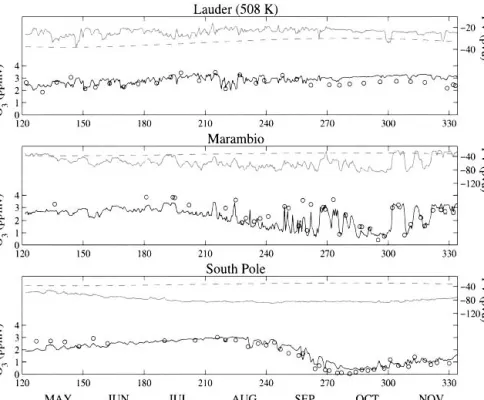
formed at various stations located in both polar and midlatitude regions. This validation is also carried out for the 2001 simulation, which is characterized by a stable and somewhat circular polar vortex, in contrast to the particular behavior of the polar vortex in 2002. Three different SH stations were selected for this analy-sis: Lauder (45.04°S, 169.68°E) located in the midlati-tudes; Marambio (64.23°S, 56.72°W) in the Palmer Pen-insula, usually close to the vortex edge; and South Pole (89.99°S,102.00°W), typically found in the center of the vortex. Figure 1 shows the evolution from 1 May to 30 November 2002 of the simulated ozone mixing ratio at 508 K compared to the measurements performed at Lauder (top), Marambio (middle), and South Pole (bottom). The 508-K level corresponds to the region of maximum polar ozone destruction in springtime. The PV and the PV threshold value corresponding to the outer boundary of the vortex are also plotted in order to track the presence of the vortex above a station that is characterized by PV values lower than the PV thresh-old value. The signature of the major warming is easily visible above a polar station like South Pole. The South Pole station usually lies deep inside the vortex but probes extravortex air during the major warming due to the displacement/elongation of the vortex.
From May to mid-July, the evolution of ozone in the polar regions is mostly controlled by the air subsidence (Rosenfield et al. 1994), which induces an increase in ozone mixing ratio under the ozone maximum and a decrease above. The effect of subsidence is weak at 508 K, due to the small vertical gradient of ozone mixing ratio at this level during that period. It is most notice-able at South Pole, where both simulated and measured ozone mixing ratios show relatively stable values of about 3 ppmv up to mid-July. The model underesti-mates ozone levels at Marambio early in the winter when polar air (low PV air) is probed. This might be due to an underestimation of the diabatic descent at the edge of the vortex during this period (Marchand et al. 2003). The onset of chemical ozone destruction starts to be visible at Marambio when the vortex moves above the station after July. The chemical ozone loss starts earlier within the vortex edge (Marambio) than within the core of the vortex (South Pole) due to its early exposure to sunlight, as shown by Lee et al. (2001). The day-to-day variability due the movements of the vortex and the polar ozone destruction are generally well re-produced by the model at both polar stations (South Pole and Marambio). The signature of the major warm-ing (last week of September) is particularly visible at
FIG. 1. Temporal evolution of the ozone mixing ratio and PV from the beginning of May to the end of Nov 2002 at 508 K at (top) Lauder, (middle) Marambio, and (bottom) South Pole for the year 2002. The black solid line shows the simulated ozone mixing ratio, the circles show the ozonesonde measurements, the gray solid line shows the PV, and the gray dashed line shows the PV outer edge of the vortex. The scale for the ozone mixing ratio is displayed on the left axis (in ppmv) and the scale for PV [in potential vorticity units (PVU) where 1 PVU ⫽ 1.0 ⫻ 10⫺6m2s⫺1K kg⫺1] is displayed on the right axis.
South Pole. The vortex moves off the pole and off South Pole during this period (from day 267 to day 278). As a result, extravortex air began to be probed over the South Pole station, as indicated by the sharp increases in both ozone and PV values. This was then followed by a rapid return to low ozone and PV levels characteristic of vortex air. The late increase in ozone observed in November at the South Pole and Maram-bio is also correctly simulated by the model and corre-sponds again to high PV values characteristic of mid-latitude air. It occurred earlier at South Pole with high ozone amounts observed from the beginning of Novem-ber, while low ozone values are still present at Maram-bio until the middle of that month. This time shift re-sulted from the displacement off the Pole of the rem-nant vortex during this period. The ozone loss derived from the difference between the model ozone passive tracer and the measured or simulated ozone at South Pole over the August–October period reaches about 2.4 ppmv according to the ozonesondes and 2.8 ppmv ac-cording to the simulations.
Several discrepancies are noticeable between the measurements and the simulations at the polar stations. At Marambio, the model underestimates ozone amounts by about 20% on average prior to the ozone destruction period (in August). The model also overes-timates ozone concentrations above the ozone maxi-mum level (not shown), which indicates an underesti-mation of the polar diabatic descent. After the major warming, the modeled ozone values are in excellent
agreement with the observations at both South Pole and Marambio particularly when the vortex is above the stations (in October at South Pole and during the first two weeks of November at Marambio). During these periods, the ozone mixing ratio stabilizes around 0.7 ppmv at South Pole and 1 ppmv at Marambio. These measured values are similar to those reported in Randall et al. (2005).
The simulated ozone time series at Lauder station shows very good agreement with the measurements at that level up to the end of October, with a mean dif-ference between simulated and observed ozone values of 7%⫾ 3% standard error. From November, the simu-lation overestimates the measured values by about 20% on average. The REPROBUS model, which is used to force the MIMOSA-CHIM model at the 30°S boundary, shows the same tendency. It appears to be linked to an overestimation of the strength of the Brewer–Dobson circulation in the ECMWF analysis. The perturbation due to the major warming is hardly visible in the evolution of PV and ozone mixing ratio over this midlatitude station, as shown in Fig. 1, from 25 September (day 268) to the end of October (day 300). During this period, the model overestimates by around 20% three measurements, whereas a good agreement between measurements and simulation is found after-ward.
Figure 2 shows the comparison between the simula-tion and ozonesonde measurements for the winter of 2001. The overall ozone evolution in 2001 can be
con-FIG. 2. Same as in Fig. 1, but for the year 2001.
trasted to the previous results in order to highlight the unusual effects of the early major warming of 2002. At Lauder, the agreement between simulations and mea-surements is again quite satisfactory. The model repro-duces correctly the day-to-day ozone variability. It shows, however, the same tendency to overestimate the observed values at the end of the period; from mid-September to the end of November, the average bias between the simulated and observed ozone values is of the order of 23%. In the case of Marambio, the 2001 simulation tends generally to underestimate the mea-sured ozone values, but the day-to-day variability is well reproduced. The average discrepancy between the simulated and observed ozone values is about 4% ⫾ 7% standard error over the whole period. The de-creases in ozone observed from the beginning of Au-gust to mid-September (day 200 to 240) for both years are comparable. Afterward, the ozone evolution at this station exhibits more variability in 2001 than in 2002. Usually, Marambio is located just on the edge of the vortex where the gradients in ozone are maximum. Consequently, small fluctuations in the position of the vortex lead to relatively large fluctuations in ozone lev-els over the station. In 2002, the movements of the vortex were so large that the station tended to remain either inside or outside the vortex for a few days instead of mostly moving within the vortex edge region like in 2001. As a result, there was less short-term variability in 2002 than in 2001.
At South Pole, the evolution in ozone is similar in both years until the major warming (last week of Sep-tember). Nonetheless, ozone levels in both simulation and observation time series are higher in 2002 than in 2001 prior to the springtime ozone destruction. It is due to a stronger diabatic descent within the vortex in 2002. In 2001, the measurements show complete ozone de-struction by the end of September, while the simulation slightly overestimates the observed values during the destruction period. In 2002, the destruction is inter-rupted by the major warming. As a result, ozone never reaches zero values at 508 K as observed during the preceding winters. Overall, the low ozone values are maintained up to the end of November in 2001, which is consistent with the particularly persistent polar vor-tex during that year. The slight increase of ozone values observed during November is correctly simulated by the model.
Finally, we focus our attention on the CTM’s ability to reproduce ozone profiles during the major warming of 2002, a period when the vortex was extremely dis-torted not only horizontally but also vertically. Figure 3 presents the comparison of simulated and measured ozone mixing ratio profiles above South Pole on 27 September and 21 October 2002, during and just after the major warming, respectively. The right-hand plots of the figure show modified potential vorticity (MPV) profiles over the station as well as the MPV threshold value corresponding to the outer boundary of the
vor-tex. MPV is PV normalized to a potential temperature level [MPV⫽ PV(/0)
(–9/2); where
0⫽ 500 K]. It is
used to remove the exponential growth of PV with height in an isothermal atmosphere (Lait 1994). An MPV value lower (or higher, if MPV is given in abso-lute value) than the MPV threshold value of the vortex outer boundary indicates that the polar vortex is above the station at the considered level. This is the case up to 500 K on 27 September and in the entire shown altitude range on 21 October. Ozone mixing ratios are correctly simulated by the model in the lower stratosphere. They are somewhat overestimated above, especially inside the vortex as seen on 21 October. The ozone profiles exhibit the same characteristics as the observed profiles inside and outside the vortex during that period. All South Pole profiles simulated and observed during the major warming show ozone amounts characteristics of the midlatitudes from 550 K upward and low ozone values in the lower stratosphere. This pattern is due to the split of the vortex in the middle stratosphere, which is caused by the major warming, as shown in Allen et al. (2003). After this perturbed period, the polar vortex ended up strongly reduced in size (Allen et al. 2003), but it returned to a more classical shape, as illustrated by the ozone profile of 21 October, where lower levels of ozone were once again observed in the middle strato-sphere.
4. Origin of vortex and midlatitude ozone loss
The particular meteorology of the 2002 Antarctic winter is expected to have led to different interactions between polar and midlatitude regions. This should re-sult in different chemical conditions, compared to pre-vious winters, with possible changes in the pathways and regions of ozone destruction. Using the range of model air tracers and ozone tracers described in section 2, we now examine the geographical origins (vortex versus extravortex) of the chemical ozone destruction. The model quantifications are provided within different equivalent latitude (EL) bands (McIntyre and Palmer 1984; Butchart and Remsberg 1986). Equivalent lati-tude is derived from the modeled PV (Lary et al. 1995). The use of EL as horizontal coordinate allows us to position the grid cells with respect to the polar vortex. The center of vortex is defined as the minimum in PV (or maximum absolute PV) and corresponds to 90°S EL. In the case of an extremely distorted vortex and of a vertical misalignment of the vortices, as seen in 2002 (Kondragunta et al. 2005), use of this coordinate system artificially realigns the vortices at different levels on top of each other. The ozone loss analysis in terms of equivalent latitude is well adapted to the 2002 winter meteorology. The geographical and chemical origins of the ozone loss column can be identified using air and chemical ozone tracers.
As the bulk of the rapid springtime ozone depletion is generally centered around 15 km, we focus here on
the lower-stratospheric partial column between 350 and ⬃510 K. The ozone analysis is performed for the 2002 and 2001 winters. The strong contrast between the me-teorologies of these two winters provides an opportu-nity to gain some insight into the influence of dynamics and, in particular, mixing of the ozone destruction in the vortex and the extravortex region.
The model-calculated components (total, vortex, and extravortex) of the accumulated ozone loss integrated over the partial column between 350 and 508 K are
plotted as a function of equivalent latitude and time in Fig. 4 and in Fig. 5 for 2002 and 2001, respectively. Note that the term ozone loss refers to the net chemical ozone loss, which is defined as destruction minus pro-duction; it is estimated from the difference between the ozone-like passive tracer and the active ozone. The top plot of each figure presents the time evolution of the total accumulated ozone loss column from 1 May to 31 December. The combination of ozone loss tracers al-lows us to differentiate between the amount of ozone
FIG. 3. (left) Model-calculated (gray line) and measured (black line) ozone profiles at South Pole on 27 Sep and 21 Oct 2002. (right) Modified PV profile (black line) and the MPV value of the vortex outer boundary (gray stars) over South Pole for the days corresponding to the left panel.
FIG. 4. (a) Model-calculated total accumulated ozone loss, (b) its vortex, and (c) extravortex contributions as a function of EL and time, from 1 May to 31 Dec 2002. The ozone loss (in DU) is integrated over the partial column 350–508 K. The thick solid black line represents the position of the vortex outer edge at 462 K.
FIG. 5. Same as in Fig. 4, but for the year 2001.
that has been destroyed within the vortex (referred to in the text as vortex ozone destruction or vortex con-tribution) from the amount that has been destroyed outside the vortex (referred to in the text as extravortex ozone destruction or extravortex contribution). Figures 4b,c and 5b,c present the time evolution of these two contributions, with the top plot being approximately equal to the sum of the two contributions. Indeed, the total ozone loss derived from the sum of the ozone loss tracers over an isentropic surface is approximately equal to the corresponding total ozone loss derived from the difference between the ozone-like passive tracer and the chemically active ozone. The evolution of the outer boundary of the vortex at 462 K is also shown in all of the plots.
a. Polar vortex region 1) TOTAL OZONE LOSS
First, we analyze the total ozone loss within the polar vortex region, which is enclosed by the outer boundary of the vortex (region poleward of about 60°S equivalent latitude). The ozone destruction starts in both simula-tions at the edge of the polar vortex region because the edge is the first part of the vortex exposed to sunlight. The ozone destruction starts earlier in 2002 compared to 2001. This suggests that the unusually strong wave activity in 2002 had an effect on ozone levels well be-fore the major stratospheric warming, especially around the vortex edge region. The resulting small dis-placements of the vortex off the Pole cause the vortex edge to be exposed to sunlight and ozone destruction earlier than in 2001. One can notice that the total ozone loss contours in Figs. 4 and 5 tend to be vertical in the inner part of the vortex region (region poleward of about 70°S equivalent latitude; also called vortex core), indicating that there is little spatial variation in ozone loss within this region. This confirms that the vortex core is a strongly mixed region (Lee et al. 2001). The vortex core covers the EL region ⬃70°–90°S during most of the 2001 simulation. It covers a similar area during the first half of 2002, but then its size decreases substantially from October onward. The total 2002 ozone loss within the deep vortex core (EL region 80°– 90°S) remains similar to the 2001 vortex core ozone loss until late November. The maximum ozone loss in 2002 is only slightly smaller than in 2001. This is consistent with the vortex core remaining intact and relatively iso-lated in the lower stratosphere during and after the major warming of late September in 2002 (Konopka et al. 2005). By the end of November, the 2002 ozone loss within the vortex core (EL region 75°–90°S) drops sharply, indicating the final breakup and dilution of remnants of the polar vortex. The 2001 ozone loss within the vortex core remains well preserved until late December.
The temporal evolution of the position in equivalent latitude of the outer boundary of the vortex at 462 K
indicates that the 2002 polar vortex starts to shrink in August. It shrinks faster from the end of September onward. The 2001 vortex starts to shrink in October, at a much slower rate than in 2002. By late November, the 2001 vortex covers an area (corresponding to the EL region⬃60°–90°S) that is approximately twice the size of the 2002 vortex (corresponding to the EL region ⬃70°–90°S). Important differences in terms of ozone losses are found in the vortex edge region, which is a broad ring of weakly mixed air surrounding the vortex core and extending out to the vortex outer boundary. Although the position of the vortex edge region in EL depends on the size of the vortex, it is typically centered around the 60°–70°S EL band in the simulations. The evolution of the ozone loss within this broad EL band is comparable in the two simulations until late Septem-ber. The ozone destruction becomes very significant in August in both simulations, with the ozone loss increas-ing steadily from then on. However, the evolutions of the ozone loss within the vortex edge region diverge very significantly at the end of September. In the 2002 simulation, the ozone loss within the vortex edge region decreases during and just after the major stratospheric warming. The ozone loss decreases even further during November. In contrast, the 2001 vortex edge zone loss continues to increase in October and November, al-though at a much slower rate than in September. It only starts decreasing in late December, at the end of simu-lation.
2) VORTEX AND EXTRAVORTEX CONTRIBUTIONS TO THE VORTEX OZONE LOSS
Figures 4b,c and 5b,c show the contributions of the ozone destruction inside and outside the vortex to the total ozone loss (as shown in Figs. 4a and 5a). As ex-pected, the ozone destruction within the vortex is by far the most important contributor to the total ozone loss within the polar vortex region for both winters (on av-erage, 92% of the total for 2002 and 98% for 2001). Nonetheless, the contribution of the extravortex de-struction (Fig. 4c) to the total ozone loss within the polar vortex region is significant in 2002. This extravor-tex contribution originates from air that experiences ozone destruction at the midlatitude region and is sub-sequently transported and mixed into the vortex region. It influences the polar vortex core (EL region 75°–90°S) from September onward, reaching about 10 Dobson units (DU; 1 DU⫽ 2.89 ⫻ 1016molecules cm⫺2) at the
end of 2002. The extravortex contribution to the total ozone loss within the vortex region is smaller in 2001 than in 2002 (on average, 2% of the total for 2001 and 8% for 2002). Its effect is only felt within the vortex edge region during most of the simulation. It slightly affects the vortex core in December. The differences in the way the extravortex destruction affects ozone loss in the vortex region reveal differences between the simulations in the mixing properties of the vortex edge region. This region is characterized by weak mixing and
usually remains isolated from the Antarctic vortex core between late winter and midspring (Lee et al. 2001). This is the case in 2001 where the extravortex ozone destruction does not affect the vortex core (bottom plot of Fig. 5). However, in 2002, the unusual wave-induced disturbances of the polar vortex clearly enhanced mix-ing within the vortex edge region. This process started to be effective well before the major stratospheric warming, which obviously weakened the vortex edge much further. The effect of the series of minor warm-ings in August and early September 2002 on the strength of mixing within the vortex edge region is also visible in the spreading of the extravortex contribution to the vortex core (see bottom plot of Fig. 4).
b. The midlatitude region 1) TOTAL OZONE LOSS
We now focus our attention on the region outside the vortex, which is contained between about 30° and 60°S equivalent latitude (referred to in the text as the mid-latitude region). The ozone destruction in the midlati-tude region is most effective near the vortex edge in both simulations. The evolutions of the total ozone loss in the midlatitudes in the two simulations start diverg-ing in early August (see Figs. 4a and 5a). The rate of ozone destruction in the midlatitudes (EL region 30°– 50°S) is 2 times higher in August and September in 2002 compared to 2001. The maximum differences in total ozone loss are also found close to the outer boundary of the vortex and reach ⬃20 DU in late September; the total ozone loss contours tend to bend toward the low latitudes during August and September in 2002 (see Fig. 4a), whereas they tend to follow the outer bound-ary of the vortex in 2001 (see Fig. 5a). This is indicative of stronger mixing in the midlatitude region during Au-gust and September in 2002 compared to 2001. The unusually strong perturbations of the polar vortex, which include the minor stratospheric warmings in Au-gust and early September in 2002, do not only enhance mixing within the vortex edge region, as shown in the previous section, but also enhance it within the midlati-tude region. The largest ozone loss values are found in the region surrounding the vortex. They start to spread to low latitudes in October in the 2001 simulation, about 2 months later than in 2002. By December, the midlatitude total ozone loss in 2001 is only about 5 DU smaller than the one in the 2002 simulation.
2) VORTEX AND EXTRAVORTEX CONTRIBUTIONS TO MIDLATITUDE OZONE LOSS
The extravortex ozone destruction is the main con-tributor to the total ozone loss in the midlatitude region until mid-September in 2002 and until October in 2001. From these dates on, the contribution of the vortex ozone destruction increases sharply and rapidly out-weighs the extravortex contribution. By the end, it
rep-resents about 80% of the total on average. The extra-vortex ozone destruction is maximum near the extra-vortex outer boundary in both simulations. The chemical com-position of this region is strongly influenced by ex-changes with the vortex and, in particular, by the export of chemically activated vortex air rich in ozone-destroying chlorine radicals.
From August onward, the extravortex contribution is more important in 2002 than in 2001. It is the result of a more permeable vortex edge in 2002 that favors the export of chemically activated polar vortex air to the midlatitude region. The magnitude of the extravortex component to the ozone loss near the vortex increases throughout the 2002 simulation to reach 15 DU (20% of total ozone loss) in December during the breakup of the vortex (see Fig. 4c). The erosion and breakup of the polar vortex from October to December 2002 supply the midlatitude region with chemically activated vortex air resulting in a more or less continuous ozone destruc-tion outside the vortex. It is worth pointing out that this fraction of ozone destruction that takes place outside the vortex has its origin in chlorine activation processes within the polar vortex. In a sense, it could also be labeled vortex ozone destruction. In contrast, the ex-travortex contribution to ozone loss starts to decrease in September in the 2001 simulation (see Fig. 5c). The vortex edge acted as an efficient barrier to mixing dur-ing 2001. Without the export of activated vortex air, the extravortex ozone destruction is limited in the 2001 simulation and is outweighed by the ozone production from the photolysis rate of molecular oxygen when the sunlight returns in the spring.
3) INDIVIDUAL OZONE-DESTROYING MECHANISMS OF THE EXTRAVORTEX CONTRIBUTION
To characterize the chemical pathways of the extra-vortex ozone destruction, the different ozone-destroy-ing components of the extravortex contribution (i.e., accumulated ozone loss from each main catalytic cycle operating in the extravortex region) are plotted as a function of time and equivalent latitude in Fig. 6 . The ozone production term (photolysis of molecular oxy-gen) is not presented because the differences between 2001 and 2002 are not significant in our analysis. The sum of the ozone-destroying terms (shown in the left-hand plots of Fig. 6 for 2002 and in the right-left-hand plots of Fig. 6 for 2001) and of the production term (not shown) is approximately equal to the extravortex con-tribution (shown in Fig. 4c for 2002 and Fig. 5c for 2001).
The extravortex ozone destruction is more intense in 2002 than in 2001, especially in the vicinity of the vor-tex. Small differences between the two simulations ap-pear very early on, in June and July. The most notice-able difference concerns the magnitude of the halogen-catalyzed ozone destruction. The halogen cycle in the 2002 simulation is the dominant ozone destruction pro-cess until September in the region surrounding the
FIG. 6. Model-calculated accumulated ozone loss (in DU) due to ozone-destroying (top) NOx, (middle) halogen,
and (bottom) HOxcatalytic cycles for the (left) 2002 and (right) 2001 extravortex contributions, which are shown
on the bottom plots of Figs. 4 and 5. The NOxcomponent represents the accumulated ozone loss due to the NO2
⫹ O cycle; the halogen component corresponds to the ClO dimer, ClO ⫹ BrO, ClO ⫹ HO2, and BrO⫹ HO2
cycles; the HOxcomponent corresponds to the HO2⫹ O3, H⫹ O3, and OH⫹ O3cycles.
tex. By that time, it is 3 times more efficient than in the 2001 simulation. The efficiency of the halogen cycle in extravortex air is mainly determined by the amount of chemically activated vortex air being exported to the midlatitude region. The 2002 anomalies in wave activity started to appear in May with an increased frequency and intensity in August and September (Allen et al. 2003). They weakened the vortex during this period and promoted mixing in the chemically activated vortex edge and its surroundings, resulting in an unusually ef-ficient halogen cycle in extravortex air in 2002. The HOxand NOxcycles are also more effective in the 2002
simulation than in the 2001 simulation. Overall, the HOxcycle is the most important cycle for ozone loss in
the midlatitudes in both simulations. The NOx cycle
becomes very significant in late October in the 2002 simulation and in December in the 2001 simulation. The efficiencies of the HOx and NOx cycles increase
very substantially after the major stratospheric warm-ing in the 2002 simulation. It is linked to the elongation/ split of the polar vortex and its erosion, which releases activated vortex air into the midlatitude region. Vortex air is older than extravortex air and therefore richer in water vapor and nitric acid, another source of HOxin
springtime conditions. The fact that the extravortex ozone destruction contours for the different cycles spread quickly to the vortex core in the 2002 simulation is due to the enhanced wave-induced mixing within the vortex edge region, as discussed previously.
5. Summary and conclusions
A three-dimensional high-resolution chemical trans-port model called MIMOSA-CHIM is used to investi-gate the regions and pathways of ozone destruction during the exceptional 2002 Antarctic winter. To iden-tify the changes from a typical Antarctic winter and estimate the influence of contrasting Antarctic meteo-rological conditions on the vortex and extravortex ozone destruction, the ozone evolution during the more typical 2001 winter is also simulated. An ozone budget analysis is performed for both simulations. The model results are evaluated against ozonesonde measure-ments at three stations located in both polar and mid-latitude regions [Lauder (45°04⬘S, 169°E), Marambio (64.23°S, 56.72°W), and South Pole (89.99°S, 102.00°W)]. The comparisons show a reasonably good agreement, although the diabatic descent in polar re-gions is found to be underestimated in early winter.
The origins (vortex versus extravortex) of ozone de-struction are estimated using a range of model air and chemical ozone tracers mapped onto equivalent lati-tude coordinates. The evolution of the model-calculated 2002 ozone loss within the deep vortex core is found to be similar to the 2001 ozone evolution until November. It is consistent with a lower-stratospheric vortex core remaining more or less isolated in 2002, even during the major stratospheric warming of late
September (Sinnhuber et al. 2003; Hoppel et al. 2003; Allen et al. 2003). However, concerning the ozone loss within the vortex edge region, the simulations start di-verging in late September. The vortex edge region is a broad ring, usually of weakly mixed air surrounding the vortex core and extending out to the vortex outer boundary. The 2002 ozone loss within this region starts decreasing in late September with a further decrease in November. It is partly linked to the extreme elongation of the vortex in late September and its subsequent ero-sion. In contrast, the 2001 vortex edge ozone loss car-ries on being preserved in October and November, re-flecting the stability and strength of the 2001 vortex. The ozone loss within the vortex decreases in late De-cember in 2001. Significant differences are also found in the extravortex region with the ozone destruction being most effective in the vicinity of the vortex due to the export of chemically activated vortex air. The evolu-tions of the extravortex ozone loss in the two simula-tions start diverging in early August. The rate of mid-latitude ozone destruction in August and September is 2 times higher in 2002 compared to 2001. This is due to the unusually strong wave activity in 2002, which had a substantial effect on the mixing properties of the vortex edge region and, to a lesser extent, of the extravortex region. Anomalies in wave activity started to appear in May. Their frequency and intensity increased in August and early September with a series of minor strato-spheric warmings (Allen et al. 2003). The effect of these perturbations is to enhance mixing well before the ma-jor warming within the vortex edge and the surrounding extravortex region in 2002. As a result of the enhanced permeability of the vortex edge, the export of chemi-cally activated vortex air is clearly more efficient in 2002 compared to 2001 with a noticeable impact on the midlatitude ozone loss. If these two contrasted meteo-rologies represent two expected regimes, then the simu-lations give a vision of expected differences in the fu-ture. If the exceptional meteorological conditions of 2002 were to become more prevalent in the future, the ozone depletion within the Antarctic polar vortex would certainly be reduced, especially in the vortex edge region. However, under those conditions, it is also likely that the polar vortex chemical activation would negatively impact midlatitude ozone much earlier in the winter. The winter ozone trends over the populated areas of the Southern Hemisphere midlatitudes are ac-tually very small (WMO 2002). A shift toward winters like 2002 should have implications for midlatitude ozone levels during the winter.
Acknowledgments. We are grateful to ECMWF and NILU for providing meteorological data. We are grate-ful to Greg Bodeker (NIWA), Petteri Taalas and Maximo Ginzburg (FMI/SMN), and Bryan Johnson and Sam Oltmans (NOAA/CMDL) for the ozone-sondes at Lauder, Marambio, and South Pole, respec-tively.
REFERENCES
Allen, D., R. Bevilacqua, G. Nedoluha, C. Randall, and G. Man-ney, 2003: Unusual stratospheric transport and mixing during the 2002 Antarctic winter. Geophys. Res. Lett., 30, 1599, doi:10.1029/2003GL017117.
Bergeret, V., S. Bekki, S. Godin, and G. Mégie, 1998: Antarctic ozone seasonal variation analysis in the lower stratosphere from Lidar and Sounding measurements at Dumont d’Urville. C. R. Acad. Sci., 326, 751–756.
Bodeker, G. E., H. Struthers, and B. J. Connor, 2002: Dynamical containment of Antarctic ozone depletion. Geophys. Res.
Lett., 29, 1098, doi:10.1029/2001GL014206.
Butchart, N., and E. Remsberg, 1986: The area of the strato-spheric polar vortex as a diagnostic for tracer transport on an isentropic surface. J. Atmos. Sci., 43, 1319–1339.
Chipperfield, M. P., 1999: Multiannual simulation with a three-dimensional chemical transport model. J. Geophys. Res., 104, 1781–1806.
Godin, S., M. Marchand, and A. Hauchecorne, 2002: Influence of the Arctic polar vortex erosion on the lower stratospheric ozone amount at Haute-Provence Observatory (43.92°N, 5.71°E). J. Geophys. Res., 107, 8272, doi:10.1029/ 2001JD000516.
Hauchecorne, A., S. Godin, M. Marchand, B. Heese, and C. Sou-prayen, 2002: Quantification of the transport of chemical con-stituents from the polar vortex to middle latitudes in the lower stratosphere using the high-resolution advection model MIMOSA and effective diffusivity. J. Geophys. Res., 107, 8289, doi:10.1029/2001JD000491.
Hoppel, K., R. Bevilacqua, D. Allen, and G. Nedoluha, 2003: POAM III observations of the anomalous 2002 Antarctic ozone hole. Geophys. Res. Lett., 30, 1394, doi:10.1029/ 2003GL016899.
Kondragunta, S., and Coauthors, 2005: Vertical structure of the anomalous 2002 Antarctic ozone hole. J. Atmos. Sci., 62, 801– 811.
Konopka, P., J.-U. Grooß, H.-M. Steinhorst, and R. Mueller, 2005: Mixing and chemical ozone loss during and after the Antarctic polar vortex major warming in September 2002. J.
Atmos. Sci., 62, 847–859.
Lait, L. R., 1994: An alternative form for potential vorticity. J.
Atmos. Sci., 51, 1754–1759.
Lary, D. J., M. P. Chipperfield, J. A. Pyle, W. A. Norton, and L. P. Riishojgaard, 1995: Three-dimensional tracer initialization and general diagnostics using equivalent PV latitude poten-tial temperature coordinates. Quart. J. Roy. Meteor. Soc., 121, 187–210.
Lee, A., H. Roscoe, A. Jones, P. Haynes, E. Shuckburgh, M. Morrey, and H. Pumphrey, 2001: The impact of the mixing properties within the Antarctic stratospheric vortex on ozone loss in spring. J. Geophys. Res., 106, 3203–3211.
——, R. L. Jones, I. Kilbane-Dawe, and J. A. Pyle, 2002: Diag-nosing ozone loss in the extratropical stratosphere. J.
Geo-phys. Res., 107, 4110, doi:10.1029/2001JD000538.
Lefèvre, F., G. P. Brasseur, I. Folkins, A. K. Smith, and P. Simon, 1994: Chemistry of the 1991–1992 stratospheric winter: Three-dimensional model simulations. J. Geophys. Res., 99, 8183–8195.
——, F. Figarol, K. S. Carslaw, and T. Peter, 1998: The 1997 Arctic ozone depletion quantified from three-dimensional model simulations. Geophys. Res. Lett., 25, 2425–2428.
Marchand, M., S. Godin, A. Hauchecorne, F. Lefèvre, S. Bekki, and M. P. Chipperfield, 2003: Influence of polar ozone loss on northern mid-latitude regions estimated by a high resolution chemistry transport model during winter 1999–2000. J.
Geo-phys. Res., 108, 8326, doi:10.1029/2001JD000906.
McIntyre, M. E., and T. N. Palmer, 1984: The “surf zone” in the stratosphere. J. Atmos. Terr. Phys., 9, 825–849.
Millard, G. A., A. M. Lee, and J. A. Pyle, 2003: A model study of the connection between polar and midlatitude ozone loss in the Northern Hemisphere lower stratosphere. J. Geophys.
Res., 108, 8323, doi:10.1029/2001JD000899.
Nash, E. R., P. A. Newman, J. E. Rosenfield, and M. E. Schoeberl, 1996: An objective determination of the polar vortex using Ertel’s potential vorticity. J. Geophys. Res., 101, 9471–9478. Prather, M., and A. H. Jaffe, 1990: Global impact of the Antarctic ozone hole: Chemical propagation. J. Geophys. Res., 95, 3473–3492.
Randall, C. E., and Coauthors, 2005: Reconstruction and simula-tion of stratospheric ozone distribusimula-tions during the 2002 aus-tral winter. J. Atmos. Sci., 62, 748–764.
Rosenfield, J. E., P. A. Newman, and M. R. Schoeberl, 1994: Computation of diabatic descent in the stratospheric polar vortex. J. Geophys. Res., 99, 677–689.
Shine, K. P., 1987: The middle atmosphere in the absence of dy-namic heat fluxes. Quart. J. Roy. Meteor. Soc., 113, 603–633. Sinnhuber, B.-M., M. Weber, A. Amankwah, and J. P. Burrows, 2003: Total ozone during the unusual Antarctic winter of 2 0 0 2 . G e o p h y s . R e s . L e t t . , 3 0 , 1 5 8 0 , d o i : 1 0 . 1 0 2 9 / 2002GL016798.
Varotsos, C., 2002: The Southern Hemisphere ozone hole split in 2002. Environ. Sci. Pollut. Res., 9, 375–376.
WMO, 1994: Scientific assessment of ozone depletion. Rep. 37. ——, 2002: Scientific assessment of ozone depletion. Rep. 47.