HAL Id: hal-01904321
https://hal.archives-ouvertes.fr/hal-01904321
Submitted on 24 Oct 2018
HAL is a multi-disciplinary open access archive for the deposit and dissemination of sci-entific research documents, whether they are pub-lished or not. The documents may come from teaching and research institutions in France or abroad, or from public or private research centers.
L’archive ouverte pluridisciplinaire HAL, est destinée au dépôt et à la diffusion de documents scientifiques de niveau recherche, publiés ou non, émanant des établissements d’enseignement et de recherche français ou étrangers, des laboratoires publics ou privés.
Montmorillonite colloids: I. Characterization and
stability of dispersions with different size fractions
Knapp Karin Norrfors, Muriel Bouby, Stephanie Heck, Nicolas Finck, Remi
Marsac, Thorsten Schäfer, Horst Geckeis, Susanna Wold
To cite this version:
Knapp Karin Norrfors, Muriel Bouby, Stephanie Heck, Nicolas Finck, Remi Marsac, et al.. Montmo-rillonite colloids: I. Characterization and stability of dispersions with different size fractions. Applied Clay Science, Elsevier, 2015, 114, pp.179 - 189. �10.1016/j.clay.2015.05.028�. �hal-01904321�
1
Montmorillonite colloids. I: Characterization and stability of dispersions
1
with different size fractions
2
Knapp Karin Norrfors*a,b, Muriel Boubya, Stephanie Hecka, Nicolas Fincka, Rémi Marsaca, Thorsten Schäfera, Horst Geckeisa
3
and Susanna Woldb
4
a: Karlsruhe Institute of Technology (KIT), Institute for Nuclear Waste Disposal (INE), P.O. Box 3640, D-760 21 Karlsruhe,
5
Germany
6
b: School of Chemical Science and Engineering, Applied Physical Chemistry, KTH Royal Institute of Technology,
7
Teknikringen 30, SE-100 44 Stockholm, Sweden
8
*Corresponding author. E-mail: norrfors@kth.se (K.K. Norrfors) Tel: +46 8 7909279. Fax: +46 8 7908772.
9
10
Abstract
11
Bentonite is planned to be used as a technical barrier in the final storage of spent nuclear fuel
12
and high level vitrified waste. In contact with ground water of low ionic strength,
13
montmorillonite colloids may be released from the bentonite buffer and thereby enhance the
14
transport of radionuclides (RNs) sorbed. In the present case, clay colloids represent
15
aggregates of several clay mineral layers. It is of major importance to determine RN sorption
16
properties for different sizes of montmorillonite aggregates, since size fractionation may
17
occur during particle transport in natural media. In this study, a protocol for size fractionation
18
of clay aggregates is developed, by sequential and direct centrifugation, in presence and
19
absence of organic matter. Seven colloidal fractions of different mean aggregate sizes are
20
obtained ranging, when considering the mean equivalent hydrodynamic sphere diameter
21
(ESD), from ~960 nm down to ~85 nm. Applying mathematical treatments (Jennings and
22
Parslow, 1988) and approximating the clay aggregates to regular disc-shaped stacks of clay
23
mineral sheets, results in mean surface diameters varying from ~1.5 µm down to ~190 nm.
24
All these colloidal fractions are characterized by XRD, IC and ICP-OES where they are found
2
to have the same chemical composition. The number of edge sites (aluminol and silanol) is
26
estimated (in mol/kg) for each colloidal fraction according to (Tournassat et al., 2003). It is
27
calculated from the mean particle sizes obtained from AsFlFFF and PCS measurements,
28
where the clay aggregates are approximated to regular disc-shaped stacks of clay mineral
29
sheets. The estimated number of edge sites varies significantly for the different clay
30
dispersions. In addition, stability studies using the various clay colloidal fractions are
31
performed by addition of NaCl, CaCl2 or MgCl2, in presence or absence of organic matter,
32
where no difference in stability is found.
33
Keywords
34
Montmorillonite colloids, characterization, size separation, number of edge sites, nuclear
35
waste disposal, colloidal stability
36
1 Introduction
37
In Swedish and Finnish repository designs (SKB, 2010; Vieno and Ikonen, 2005), high level
38
nuclear waste is foreseen to be placed in massive metal canisters, surrounded by a large
39
volume of natural or compacted bentonite as a barrier. The functionality of the clay is
40
primarily to stabilize the canister in case of movements in the bedrock and to seal small
41
fractures in the vicinity of the canister. The barrier is planned to prevent corrosive elements
42
from the surrounding, such as sulfide, thiosulfate and polythionates (Macdonald and
Sharifi-43
Asl, 2011) to come in contact with the canister. In case of canister failure, the barrier should
44
retard radionuclides (RNs) present in the spent nuclear fuel to be transported through the
45
geosphere towards the biosphere. Due to its high swelling pressure, cation exchange capacity
46
and retention properties, bentonite has an excellent buffer capacity (Karnland et al., 2006).
47
The main mineral component in bentonite is montmorillonite, an Al-rich smectite. Smectites
48
are intrinsically small particles, whereby they can be of colloidal sizes (i.e. particles of 1 nm -
3
1 µm in at least one dimension in dispersion (Stumm, 1993)). In this work, the term clay
50
colloids refer to aggregates, consisting of stacks of several clay mineral layers.
51
Over the estimated lifetime of the storage (i.e. 1 million years) in northern countries such as
52
Sweden and Finland (SKB, 2010), cycles of glaciations can be expected. In the worst case
53
scenario expected in Sweden, a large amount of glacial melt water will be transported through
54
fractures in the bedrock, down to repository depth and displace the old ground water that has
55
equilibrated with mineral surfaces for a very long time. Glacial melt water has a chemical
56
composition with low ionic strength, different from the original porewater. The chemical
57
composition of future glacial melt water is assumed to be similar to glacial melt waters of
58
today. It can be simulated by water types of pH 8-9 and low ionic strength, i.e. 5·10-4 M in the
59
worst case scenario cited above (Brown, 2002). The montmorillonite colloid stability is
60
known to increase with decreasing ionic strength, as demonstrated in several laboratories and
61
field experiments studies over a few months’ timeframe (Geckeis et al., 2004; Missana et al.,
62
2003; Schäfer et al., 2012) and can also be calculated from the DVLO-theory (Liu et al.,
63
2008). In contact with glacial melt water, the bentonite barrier may release montmorillonite
64
colloids that can be transported away from the barrier through the geosphere. In case of large
65
mass loss, the buffer functionality will be endangered. Also, in the case of a canister failure,
66
the transport of RNs can be enhanced, when transported by mobile montmorillonite colloids
67
(Möri et al., 2003).
68
Physically, colloid mobility depends strongly on the geometry of the fractures in the bedrock,
69
where fracture size distribution, surface roughness and surface charge are the most important
70
characteristics (Darbha et al., 2010; Filby et al., 2008). Chemically, the colloid mobility is
71
influenced by the mineral composition of the fracture filling material (FFM) and the pore
72
water matrix. The colloid mobility is also dependent on physical and chemical properties of
73
the clay aggregates themselves, i.e. the size heterogeneity, mineral composition and surface
4
charge. The physical and chemical properties of the bedrock are specific for each fracture,
75
though in general a separation of particles according to their size during transport is expected
76
in most systems. In a clean fracture system, i.e. fractures with low amount of FFM, and with a
77
high water velocity, a laminar flow is expected and transport of all colloid sizes is expected
78
more or less equally due to their ability to be transported with the water flow (Huber et al.,
79
2012). In contrary, if the fracture contains a larger amount of FFM, it will act as a porous
80
material, where the larger particles can be transported faster as a result of size exclusion
81
effects, sticking, clogging etc. Due to the possible particle size separation in bedrock
82
fractures, the size of the montmorillonite aggregates produced and their stability are important
83
parameters for RN transport. The thermodynamic and kinetic strength of RN-colloid
84
interaction determine the potential flux of radiotoxic waste components through the
85
geosphere. In fact, those RNs being weakly bound to colloids or showing a relatively fast
86
desorption from colloids will most likely not be carried by the montmorillonite colloids but
87
will be sorbed by the mineral surfaces instead (Huber et al., 2014).
88
Simplified models of RN and clay colloid transport are currently used in safety assessments
89
for estimating the RN transport, but presently they do not take into consideration the size
90
heterogeneity of the clay aggregates (Vahlund and Hermansson, 2006). Consequently, one
91
may wonder whether normalized sorption coefficients (KD) for RNs are valid expressions for
92
quantifying RN-montmorillonite interactions, since the ratio is given for a mean particle size
93
distribution and do not take into account polydispersity. An alternative, and perhaps better,
94
expression for quantifying the sorption capacities of surface complexed RNs is to take into
95
consideration the amount of edge sites in the colloidal dispersions. With this treatment,
96
eventual size dependent differences will be taken into account. This is valid as long as the
97
smaller particles are miniatures of the larger clay mineral particles, which may not be the case
98
for nanosized particles (Bergaya et al., 2006). Note that this approach is not adapted for RNs
5
sorbing by cation exchange (i.e. Cs+, Sr+ etc.). Large differences in surface structure between
100
larger and smaller clay particles may also be reflected in macroscopic properties, such as
101
colloidal stability (Bessho and Degueldre, 2009). In modeling, transport of RNs may be
102
under- or overestimated (Wold, 2010), e.g. the KD-values are not accurate if only the smaller
103
aggregates are transported and not the larger ones, or vice versa. Normalizing sorption
104
capacity to the number of edge sites might improve transport calculations of RNs sorbed to
105
different clay aggregate sizes. Furthermore, this treatment of KD-values could be implemented
106
to other systems, such as metal complexation to particles and their retardation in soils, as well
107
as colloidal transport in soil and surface waters (Gao et al., 1997; Lee et al., 2001; Nakamaru
108
and Uchida, 2008; Oliver et al., 2006). In addition to questionable normalization of sorption,
109
i.e. KD-values in transport modelling, there is a lack of sorption and desorption kinetic data
110
for RNs onto different size fractions of montmorillonite aggregates which should be
111
implemented for improved safety assessments calculations (Wold, 2010).
112
The aim of this work is to develop a method to separate montmorillonite aggregates into
113
defined size fractions, to characterize these fractions and finally to determine if the mean clay
114
aggregate size has any influence on the colloidal stability of montmorillonite. We describe the
115
protocol used to obtain different size fractions, a protocol which may be applied to any type of
116
clay dispersions. In addition, characterization of the different clay aggregate fractions such as
117
mean size, concentration, and the chemical composition of the colloidal dispersions is
118
presented. Furthermore, we describe stability studies performed on the colloidal fractions in
119
order to investigate the influence of ions which can be present in glacial melt water (Na+,
120
Ca2+, Mg2+ (Missana et al., 2003)) or degraded organic matter (Bhatia et al., 2010). In
121
separate studies (Norrfors et al., 2015), we investigate the RNs sorption/desorption behavior
122
in presence of these clay aggregate size fractions.
123
2 Material and Methods
6
2.1 Clay, organic matter, chemicals, synthetic ground water
125
All samples are prepared with ultra-pure water (Milli-Q system, 18.2 MΩ/cm resistivity) and
126
chemicals of reagent grade. The source of silicon was a standard solution of Si in H2O (1000
127
mg/L, Spex Certiprep). The Wyoming MX-80 bentonite from American Colloid Co. is used
128
as starting material for all experiments without any pretreatment. The MX-80 contains
129
approximately 82% montmorillonite with the structural formula:
130
Na0.30(Al1.55Fe0.21Mg0.24)(Si3.96Al0.04)O10(OH)2, Mw = 372.6 g/mol (Karnland et al., 2006) and
131
has a cation exchange capacity (CEC) of approximately 0.75 meq/g (measured according to
132
(Meier and Kahr, 1999)).
133
The fulvic acid (FA-573) used as organic matter in this study was extracted from a natural
134
ground water (Gohy573) originating from the Gorleben site, Germany (Wolf et al., 2004) and
135
subsequently purified and characterized. A detailed description can be found in (Wolf et al.,
136
2004). The elemental composition of the FA used in this work is as follows (Wolf et al.,
137
2004): C: (54.1 ± 0.1) %, H: (4.23 ± 0.08) %, O: (38.94 ± 0.04) %, N: (1.38 ± 0.02) % and S:
138
(1.32 ± 0.01) %. The proton exchange capacity is 6.82 ± 0.04 meq/g. In this study, a small
139
amount of FA is weighted, dispersed in NaOH and diluted in the corresponding initial clay
140
stock dispersions as described below. The dissolved organic carbon content is measured with
141
a TOC analyser (TOC-5000, Shimadzu).
142
A synthetic carbonated ground water (SGW) is prepared in order to simulate a glacial melt
143
water of low ionic strength. In the present case, we tend to the composition of the granitic
144
groundwater coming from the Grimsel Test Site (Geckeis et al., 2004; Möri et al., 2003). This
145
is done by mixing the requested amounts of the different salts (NaOH, NaCl, CaCl2, MgCl2,
146
NaF, Na2SO4 and NaHCO3) and an aliquot of the Si standard solution in ultra-pure water. The
147
final composition of the SGW is the following: Na+ (28.4 mg/L, 1.2 mM), Ca2+ (1.49 mg/L,
148
0.05 mM), F- (2.8 mg/L, 0.1 mM), Cl- (2.64 mg/L, 0.074 mM), SO42- (4.13 mg/L, 0.04 mM),
7
Si (0.014 mg/L, 0.5 µM) and HCO3- (84 mg/L, 1.4 mM). The ionic strength is below 2∙10-3 M
150
and the pH is 8.4 ± 0.1.
151 152
2.2 Fractionation by sequential and direct (ultra-)centrifugation
153
50 g of unpurified MX-80 bentonite is added to 5 L SGW (10 g clay/L). The dispersion is
154
regularly stirred during one day and then let to settle during three days in order to remove the
155
larger clay fractions and accessory mineral phases. After sedimentation the top 4 L are
156
isolated. It constitutes the colloidal dispersion S0. The residual solid phase (named R0) is
157
stored for further studies (Figure S1 in the supporting information file 1 (SIF-1)). Sequential
158
centrifugation (Thermo Scientific Centrifuge 2.0, with 50 mL PE centrifugation tubes, VWR,
159
Germany) or ultra-centrifugation (Beckmann Ultracentrifuge, XL90, with 100 mL Quick-seal
160
centrifuge tubes, Beckmann) is then performed at increasing speeds and times to obtain
161
various clay colloidal dispersions, starting from the supernatant S0 similarly to the protocol
162
presented in (Perret et al., 1994). The resulting supernatant after the first centrifugation step
163
corresponds to the colloidal dispersion S1 and the corresponding solid residual, R1.
164
Thereafter, the sequential centrifugation is repeated three times, where the last centrifugation
165
step is an ultra-centrifugation, leading to the supernatant S3.5. A schematic diagram for the
166
fractionation protocol is presented in the supporting information file 1, SIF-1, Figure S2. The
167
corresponding centrifugation times and speeds are summarized in Table 1. Higher
168
centrifugation speeds (up to 235 000 g) and filtrations (see SIF-2) are tested but result in
169
removing a too large part of the clay particles. Consequently, only the fractions S0 to S3.5 are
170
used in the present work.
171
In addition to the sequential centrifugation, and for comparison, two supernatants (noted with
172
the prefix UC and UC, FA) are collected directly from the supernatant S0 after only one
ultra-173
centrifugation step, using the same speed and time as the ones used to obtain the dispersion
8
S3.5. For that purpose, an initial supernatant S0 is collected after 1 day stirring and 3 days
175
sedimentation as described above, in presence (UC, FA) or absence (UC) of 11.8 mg/L FA.
176
Finally, the truly dissolved concentrations of Si, Al, Ca, Mg and Fe in equilibrium with clay
177
minerals are those determined after the strongest centrifugation step (1h at 235 000 g, SIF-2).
178
To determine the amount of each element in the clay particles, the truly dissolved
179
concentration is subtracted from the total concentration measured in the dispersion.
180
181
Table 1: Conditions for fractionation of the clay dispersions, and clay aggregate sizes expected in the
182
residuals (Ri) and in the supernatants (Si).
183
Dispersion
Conditions of separation (C: centrifugation; UC: ultracentrifugation)
Size expected in the ith residual clay fraction (Ri)
in nm
Size expected in the ith supernatant (Si) in nm S0 3 days sedimentation 1000 ≤ R0 0 ≤ S0 ≤ 1000 S1 C: 30 min (S0) at 313 g 450 ≤ R1 ≤ 1000 0 ≤ S1 ≤ 450 S2 C: 1 h (S1) at 700 g 200 ≤ R2 ≤ 450 0 ≤ S2 ≤ 200 S3 C: 4 h (S2) at 1200 g 70 ≤ R3 ≤ 200 0 ≤ S3 ≤ 70 S3.5 UC: 30 min (S3) at 26 000 g 50 ≤ R3.5 ≤ 70 0 ≤ S3.5 ≤ 50 S3.5UC UC: 30 min (S0) at 26 000 ga 50 ≤ R3.5UC 0 ≤ S3.5UC ≤ 50 S3.5UC, FA UC: 30 min (S0) at 26 000 ga 50 ≤ R3.5UC, FA 0 ≤ S3.5UC, FA ≤ 50 a: one step ultra-centrifugation from a colloidal dispersion S0 obtained after stirring and sedimentation of a
184
MX80 dispersion at 10 g/L in presence or absence of 11.8 mg/L FA .
185
The pH of all isolated supernatants is measured over a four months’ time period and remains
186
stable at 9.4 ± 0.2. All the collected supernatants and solid residues are stored at +4°C in
187
darkness before characterization and use in stability studies.
188
2.3 Characterization of the clay colloidal dispersions
9
2.3.1 Ion and clay particle concentrations determination
190
The element compositions are determined in all dispersions over time by Ion Chromatography
191
(IC, ICS-3000) and ICP-OES (Optima 2000 DV, PerkinElmer). The samples are acidified
192
before the ICP-OES measurements in 2% HNO3 (Merck, ultrapure) plus a drop of HF (Merck,
193
suprapure, 48%).
194
2.3.2 Mineral phase composition
195
Mineral phases composing the clay particle dispersions and the solid residues are determined
196
by XRD. The aim is to detect possible differences in the composition between the different
197
size fractions. XRD data are collected on residuals and supernatants prepared as oriented
198
samples obtained by drying on sample holders (low background Si wafers). The residuals are
199
prepared by dilution of the solid-gel like dispersions in ultra-pure water. The SGW alone is
200
also analyzed as a reference to identify any phase that could precipitate in the supernatants or
201
residuals upon drying. X-ray diffractograms for all samples (raw MX-80, the supernatants and
202
the residues) are also collected after saturation with ethylene glycol (SIF-4). Powder
203
diffractograms are recorded with a D8 Advance (Bruker) diffractometer (Cu Kα radiation)
204
equipped with an energy dispersive detector (Sol-X). The phases are identified with the
205
DIFFRAC.EVA version 2.0 software (Bruker) by comparison with the JCPDS 2 database.
206
2.3.3 Content of organic matter
207
The total amount of organic carbon in the dispersions prepared in presence of FA is measured
208
with a TOC analyser (TOC-5000, Shimadzu). A change in the FA concentration is obtained
209
after ultra-centrifugation (final [FA] = 8.3 mg/L compared to 11.8 mg/L initially). This result
210
indicates that a third of the organic matter might be associated with the clay aggregates while
211
most of the FA (two thirds) remains in the dispersion under the present experimental
212
conditions, as expected for these small-sized molecules and at the present pH.
10
2.3.4 Size distribution measurements
214
The size distributions of montmorillonite aggregates in all dispersions are determined by
215
Photon Correlation Spectroscopy (PCS, homodyne single beam ZetaPlus System equipped
216
with a 50mW solid-state laser emitting at 632 nm, Brookhaven Inc, USA) and Asymmetric
217
Flow Field-Flow Fractionation system (AsFlFFF, HRFFF 10.000 AF4, Postnova Analytics,
218
Landsberg, Germany) coupled to a UV-Vis. detector (LambdaMax LC Modell 481, Waters,
219
Milford, USA) and an Inductively-Coupled Plasma-Mass Spectrometer (ICP-MS, X–Series2,
220
Thermo Scientific, Germany).
221
AsFlFFF/UV-Vis./MALLS/ICP-MS has previously been used for characterization of natural
222
or synthetic clays colloids (Bouby et al., 2012; Bouby et al., 2011; Bouby et al., 2004; Finck
223
et al., 2012; Plaschke et al., 2001). In this study, the clay dispersions obtained after
224
fractionation (Si) . are diluted to ~20 mg/L clay particles in SGW before injection into
225
the system. Details on the equipment, the fractionation conditions and the calibration are
226
given in the supporting information file (SIF-3).
227
For the PCS measurements, the clay dispersions are diluted to 10 mg/L in a disposable plastic
228
cuvette and measured over 5 runs consisting of 10 measurements of 15 s each, i.e. 50
229
measurements, for determination of mean hydrodynamic diameters.
230
231
2.4 Clay particle stability studies
232
Stability studies are performed using PCS-measurements according to the experimental
233
protocol described in (Behrens et al., 2000; Czigány et al., 2005; Holthoff et al., 1996;
234
Kretzschmar et al., 1998). The particle stability ratios (W) are calculated from the initial
11
agglomeration rates. The stability ratio is defined as the ratio between the fast agglomeration
236
rate to the measured agglomeration rate in the present sample:
237 𝑊 = → / ( ) → / Equation 1 238
where rh is the hydrodynamic radius (nm), t the time (s) and C the particle concentration
239
(mg/L), the suffix f represents the fast agglomeration rate. Equation 1 is derived from the
240
following Equations 2 and 3:
241
→ = 𝛽𝑘𝐶 Equation 2
242
𝑊 = ( ) = Equation 3
243
where is an optical factor (depending on the scattering angle, the wavelength of the light
244
and the particle radius), k is the agglomeration rate and is the particle-particle attachment
245
efficiency and so-called the sticking probability. Consequently, W approaches 1 when the
246
particles are unstable under the chemical conditions tested, while for stable dispersions, W
247
tends to go to infinity (set arbitrarily to 101-102 values in our experiments to fit into the
248
graphs).
249
In this study, W is determined at pH 7, while the ionic strength was varied between 0.01 and 3
250
M by using the electrolytes NaCl, CaCl2 or MgCl2. In addition, experiments in presence or
251
absence of FA are performed, since FA is known to stabilize montmorillonite particles
252
(Furukawa and Watkins, 2012). The clay particle concentration is fixed to 10 mg/L by prior
253
dilution throughout all measurements, and all the supernatants listed in Table 1 are studied.
254
The initial intensity-weighted hydrodynamic mean diameter is measured first during 45 s
255
before addition of the electrolyte to the dispersion. Thereafter, the evolution of the particle
256
hydrodynamic diameter is monitored, after affecting the dispersion by simultaneous addition
12
of concentrated electrolyte aliquots (NaCl, CaCl2 or MgCl2) and NaOH to reach the desired
258
chemical conditions. All samples are measured up to between 20 and 40 min after addition of
259
the electrolyte, with measurements of 15 s each. To investigate the effects of addition of FA, a
260
final concentration of 10.2 mg FA/L is added to all clay dispersions. Thereafter, 0.1 M CaCl2
261
is added to the dispersions and the results are compared to measurements in absence of FA.
262
As the pH cannot be monitored at the same time in the cuvette used for the PCS measurement,
263
it is measured in parallel in a second cuvette with a dispersion of identical composition.
264
The initial agglomeration rate is determined by fitting a second-order polynomial to the
265
experimental data, using the first 15-35 data points of each set of data. The initial
266
agglomeration rates are then compared and normalized to the fastest initial agglomeration rate
267
(determined for each electrolyte at 3M IS) for each colloidal fraction to obtain the
268
corresponding W value.
269
270
3 Results and Discussion
271
3.1 Characterization of the clay colloidal dispersions
272
3.1.1 Ion and colloid concentrations
273
The concentrations of all analyzed elements are presented in Table 2, where the mean values
274
obtained from several measurements are given. The clay colloid concentrations ([Coll.]) are
275
calculated from Al-concentrations according to the theoretical structural formula (Karnland et
276
al., 2006). The molar ratios of the different elements are calculated from the ICP-OES- and
277
IC-results and may be compared to the theoretical values based on the assumed stoichiometry.
278
Table 2: Element and colloid concentrations in the clay colloidal dispersions measured by ICP-OES and
279
IC and colloidal fraction distributions calculated from the mean concentration of four main and minor
280
clay constituents (Si, Al, Mg, and Fe). The recovered amount of colloids in the dispersions is presented as
13
percentage compared to the initial colloidal concentration in S0. *: This corresponds to the amount of
282
stable colloids in the dispersions after letting settle the dispersions during 2 months without any shaking.
283
The elemental mole ratios are corrected by the free aqueous concentrations determined after the strongest
284
ultracentrifugation, which are 7.5∙10-5 M Si, 4.1∙10-6 M Mg, 7.2∙10-7 M Fe, 3.7∙10-6 M Al and 8.5∙10-6 M Ca.
285 Dispersion [Coll.] mg/L [Al] mg/L [Mg] mg/L [Si] mg/L [Fe] mg/L [Ca] mg/L [Na] mg/L [F] mg/L [SO4] mg/L [Cl] mg/L S0 1127 ± 170 133 ± 20 20 ± 2 382 ± 110 32 ± 2 8.6 ± 0.5 87 ± 1 2.9 ± 0.5 37 ± 3 5 ± 1 S1 746 ± 68 88 ± 8 13.6 ± 0.4 252 ± 70 21.4 ± 0.6 5.7 ± 0.1 82 ± 2 2.9 ± 0.5 37 ± 3 3.9 ± 0.3 S2 551 ± 34 65 ± 4 9.9 ± 0.6 178 ± 46 15 ± 2 4.0 ± 0.2 76 ± 2 2.9 ± 0.5 37 ± 4 3.9 ± 0.4 S3 280 ± 26 33 ± 3 5.5 ± 0.2 99 ± 25 8 ± 1 2.5 77 3.0 ± 0.4 37 ± 4 3.8 ± 0.2 S3.5 96 ± 6 11.3 ± 0.6 1.9 ± 0.1 40 ± 18 2.7 ± 0.1 1.1 73 2.9 36 3.6 S3.5UC 90 ± 6 10.6 ± 0.6 1.8 ± 0.1 40 ± 18 2.8 ± 0.3 1.0 74 2.7 36 4.7 S3.5UC, FA 125 ± 3 14.7 ± 0.3 2.5 ± 0.1 51 ± 18 3.5 ± 0.1 1.6 75 3.0 36 4.8 SGW 1.6 28 2.5 3.2 2.9 Dispersion Si/Al mole ratio Al/Mg mole ratio Al/Fe mole ratio Al/Ca mole ratio Mg/Fe mole ratio Recovered colloids (%) S0 2.7 6.0 8.6 23.9 1.4 100 ± 0 (43 ± 1*) S1 2.7 5.9 8.5 24.4 1.5 67 ± 4 (47 ± 2*) S2 2.6 6.0 9.0 26.4 1.5 48 ± 5 (43 ± 2*) S3 2.8 5.5 8.6 22.7 1.6 25 ± 2 (22 ± 1*) S3.5 3.0 5.6 8.7 22.0 1.6 9.4 ± 0.1 S3.5UC 3.2 5.6 7.9 23.8 1.4 9.0 ± 0.2 S3.5UC, FA 3.1 5.5 8.7 17.3 1.6 12.1 ± 0.1 Theoretical values 2.49 6.62 7.57 1.14 286
14
As expected, the montmorillonite colloid concentration decreases with the number of
287
sequential centrifugation steps, for increasing centrifugation speed and time (Table 2). There
288
is no doubt that the particles consist of montmorillonite in all dispersions as the Si/Al, Al/Mg,
289
Al/Fe and Mg/Fe mole ratios are in fair agreement with those obtained from the theoretical
290
structural formula of montmorillonite (Table 2). Molar element ratios in the clay fraction are
291
corrected for the free aqueous concentration of dissolved elements in the dispersions. These
292
free aqueous concentrations are obtained from the supernatant of a sample centrifuged at 235
293
000 g where all clay mineral particles are assumed to be removed (SIF-2). The calcium
294
concentrations in the dispersions decrease with increasing numbers of centrifugation steps
295
similar to the decrease of colloid concentrations (Table 2) suggesting its association to the
296
clay aggregates, possibly due to ion exchange binding at the permanently charged basal plane.
297
Even though calcium does not appear in the theoretical formula, it is known that unpurified
298
MX80 bentonite contains calcium based accessory minerals, like calcite (Bradbury and
299
Baeyens, 2002; Karnland et al., 2006; Vuorinen and Snellman, 1998).
300
In addition, the results show a direct release of several elements from the unpurified bentonite
301
to the SGW, which is here the background electrolyte (Table 2). A drastic increase of sodium
302
and sulfate and, to a lower extend, fluoride and chloride is observed as already reported in the
303
literature (Bradbury and Baeyens, 2002; Vuorinen and Snellman, 1998). This can be
304
explained, altogether, by the presence of NaCl (1.35 mmol/kg), fluorite (CaF2), gypsum
305
(CaSO4) and celestite (SrSO4) in the unpurified MX80 (Bradbury and Baeyens, 2002;
306
Vuorinen and Snellman, 1998). The dissolution of NaCl from the unpurified starting material
307
cannot explain the large increase of sodium concentration in the supernatants. In addition, no
308
increase in Ca concentration is observed (the concentration of Sr is not measured). Cation
309
exchange reactions, where divalent cations (Ca/Sr) are favored over monovalent ones (Na),
310
may explain why the Na release is enhanced and no variation in Ca concentration is observed
15
(Gaucher et al., 2009). Another process involving dissolution of pyrite, which is found in the
312
XRD analysis (Figure 1), can explain the release of sulfate. However, this should be
313
accompanied by a drop of pH. Thus, it is not considered as the most important process.
314
3.1.2 Colloidal distribution in the montmorillonite fractions and long-term stability of
315
the dispersions
316
The mean clay colloidal concentrations after each centrifugation are calculated from the
317
concentrations obtained for the four main and minor montmorillonite constituents (Si, Al, Mg,
318
and Fe). They are compared to the initial concentration of colloids, which allows determining
319
the colloidal recoveries, Table 2.
320
From the total amount of colloids initially present in S0, approx. 9 % remain in the dispersion
321
S3.5 (Table 2) which is the dispersion obtained at the last fractionation step after using 27 000
322
g centrifugation. The similarity of the results obtained after one direct
ultra-323
centrifugation step (S3.5UC, 9.0 ± 0.2 %) is noticeable. A slightly higher recovery of clay
324
colloids is obtained in presence of fulvic acids (S3.5UC,FA, 12.1 ± 0.1 %), which indicates that
325
the negatively charged FA may have stabilized a part of the montmorillonite colloids initially
326
present in dispersion (Furukawa and Watkins, 2012; Kretzschmar et al., 1998).
327
To determine the long-term stability of the dispersions, the same analyses were performed 2
328
months later, without any shaking during that time or prior to the sampling. It is found that
329
not all dispersions are stable over time. This is particularly true for the dispersions S0 and S1
330
as indicated by the percentage of colloids recovered after 2 months (Table 2, marked with *)
331
showing that 57 % and 26 % of the clay colloids, respectively, have sedimented during this
332
time period. This indicates that these dispersions contain various sizes fractions, from large to
333
smaller clay aggregates, as expected from the sequential separation protocol.
334
3.1.3 Mineral phase composition
16
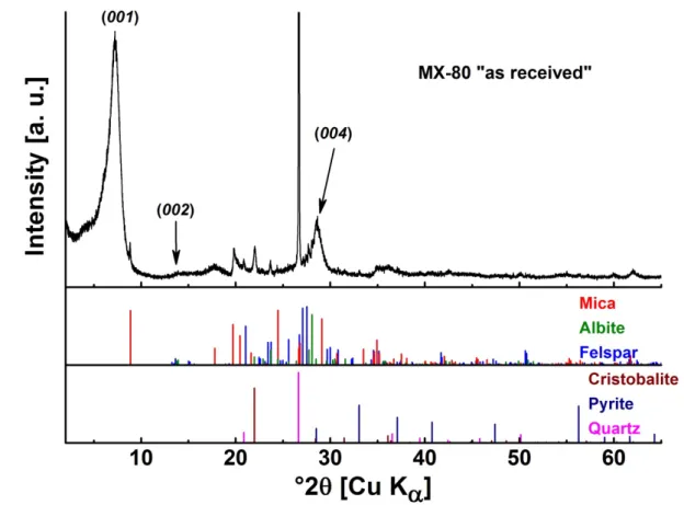
The as-received material, MX-80, consists mainly of montmorillonite, as indicated by the
336
corresponding X-ray diffractogram (Figure 1). Accessory minerals are present in the
337
unpurified bentonite such as quartz, cristobalite and mica, as well as trace amounts of albite,
338
feldspar and pyrite. No attempt was made to quantify their content. This bentonite
339
composition agrees well with reported data (Hu et al., 2009).
340
341
Figure 1: X-ray diffractogram of the as-received MX-80 and identification of the accessory minerals by
342
comparison with database. Montmorillonite 00l planes are indicated in brackets.
343
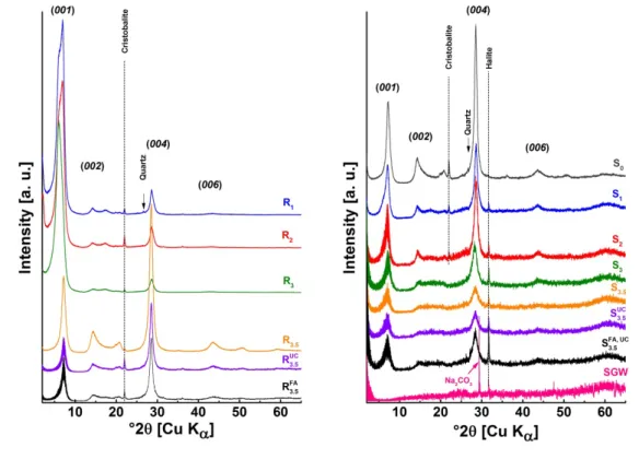
The supernatants and residuals are all analyzed after each fractionation step (Figure 2). The
344
solid material in R0 has identical mineralogical composition as the raw material. Obviously,
345
the accessory phases settled down during the first fractionation step resulting in that
346
cristobalite is detected only in the first sample and that quartz can be detected only in S0 and
347
R1. All samples, both residuals and supernatants, exhibit intense reflections at 12.2–14.6 Å
348
(7.2–6.0° 2θ) and ~3.14 Å (28.6° 2θ) corresponding to 001 and 004 reflections of
17
montmorillonite. The 001 reflection or basal spacing (i.e. d(001)), which corresponds to the c
350
dimension of the elemental unit cell, is dependent on the hydration state (Ferrage et al., 2005;
351
Meunier, 2005). In this study, all supernatants and residuals have a basal spacing
352
corresponding to the presence of one (12.2 Å) and two water molecules (14.6 Å) in the
353
interlayer. In R1 and R2, the clay is obviously heterogeneous in the hydration state as both
354
states may be present as shown by the broad 001 reflection. The clay interlayer hydration state
355
depends on the layer charge and the ambient relative humidity, not on the fractionation
356
procedure. All samples also exhibit less intense 00l reflections typical of clay minerals, such
357
as 002 and 006. Finally, all residues have a similar mineralogical composition except the
358
quartz detected in trace amounts in R1. Likewise, all suspended particles in supernatants have
359
a similar mineralogical composition, except S0, S1 and S2 that contain cristobalite and S0 that
360
contains additionally trace amount of quartz. Finally, only halite (NaCl) and Na2CO3 could be
361
detected in SGW meaning that these phases crystallized upon drying. Halite could be detected
362
in some supernatants. None of these phases (NaCl or Na2CO3) could be detected in the
363
residues.
364
All supernatants and residuals exhibit similar basal spacing after saturation with ethylene
365
glycol (SIF-4). The expansion to 17.0 ± 0.2 Å for d(001) is typical of smectite swelling, and
366
thus consistent with montmorillonite being the main component of MX-80.
18 368
Figure 2: X-ray diffractograms for all residuals (left) and supernatants (right) obtained by fractionation.
369
One can see the similarities between the residuals and supernatants, which implies a similar structure of
370
the montmorillonite in the different samples. In addition, a decrease in accessory minerals with the
371
number of centrifugation steps is seen. The montmorillonite 00l planes are indicated in brackets.
372
3.1.4 Clay aggregate size distribution measurements
373
3.1.4.1 AsFlFFF
374
Since aluminium is one of the main components of montmorillonite, the Al-data obtained
375
from the AsFlFFF/ICP-MS-measurements are used as a clay indicator. All Al-ICP-MS data
376
are presented in Figure 3 after transformation of fractograms in mass versus size by using 1)
377
the mass calibration method (left side, Figure 3a) as developed before in previous studies
378
(Bouby et al., 2008) and 2) the size calibration (right side, figure 3b), according to (Schimpf
379
et al., 2000).
19 381
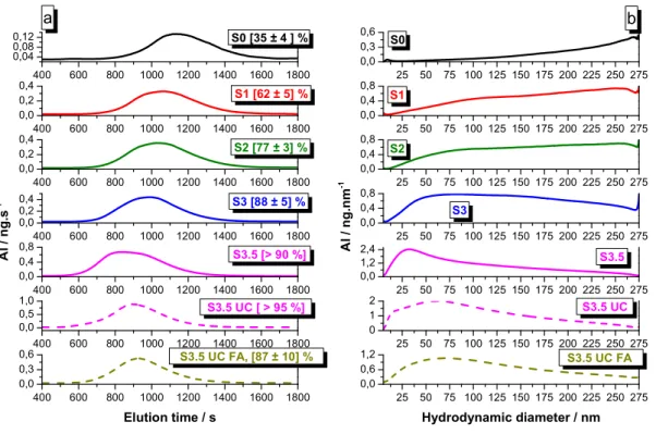
Figure 3: Al-ICP-MS fractograms obtained after injection (100 µL) of the different clay dispersions, all
382
diluted to 20 mg/L clay prior to injection. Left: fractograms transformed using the calibration in mass
383
concentration as a function of elution time (Bouby et al., 2008). Right: fractograms further transformed
384
by using the calibrations to size (Schimpf et al., 2000). The percentage in bracket indicates the colloid
385
recovery in the measurements. These are all smoothed data and a mean result of two measurements.
386
At a first look, a broad size distribution is obtained for each dispersion, ranging from 10 up to
387
275 nm. Some shoulders are clearly visible in the fractograms, indicating the presence of
388
different size fractions in the dispersions. A separation into different well-resolved size
389
fractions is not achieved due to the conditions selected for the AsFlFFF measurements (see
390
SIF-3). Nevertheless, the fractograms show clearly that the mean size of the aggregates in the
391
dispersions is decreasing with the number of fractionation steps. This is clearly evidenced by
392
the significant variation of the fractogram maxima and the mean sizes of the different
393
colloidal dispersions (Figure 3 and Table 3).
394 400 600 800 1000 1200 1400 1600 1800 0,04 0,08 0,12 S0 [35 ± 4 ] % 400 600 800 1000 1200 1400 1600 1800 0,0 0,2 0,4 S1 [62 ± 5] % 400 600 800 1000 1200 1400 1600 1800 0,0 0,2 0,4 S2 [77 ± 3] % 400 600 800 1000 1200 1400 1600 1800 0,0 0,2 0,4 A l / n g .s -1 S3 [88 ± 5] % 400 600 800 1000 1200 1400 1600 1800 0,0 0,4 0,8 S3.5 [> 90 %] 400 600 800 1000 1200 1400 1600 1800 0,0 0,5 1,0 S3.5 UC [ > 95 %] 400 600 800 1000 1200 1400 1600 1800 0,0 0,3 0,6 S3.5 UC FA, [87 ± 10] % Elution time / s a 25 50 75 100 125 150 175 200 225 250 275 0,0 0,3 0,6 S0 25 50 75 100 125 150 175 200 225 250 275 0,0 0,4 0,8 S1 25 50 75 100 125 150 175 200 225 250 275 0,0 0,4 0,8 S2 25 50 75 100 125 150 175 200 225 250 275 0,0 0,4 0,8 A l / n g .n m -1 S3 25 50 75 100 125 150 175 200 225 250 275 0,0 1,2 2,4 S3.5 25 50 75 100 125 150 175 200 225 250 275 0 1 2 S3.5 UC 25 50 75 100 125 150 175 200 225 250 275 0,0 0,6 1,2 S3.5 UC FA Hydrodynamic diameter / nm b
20
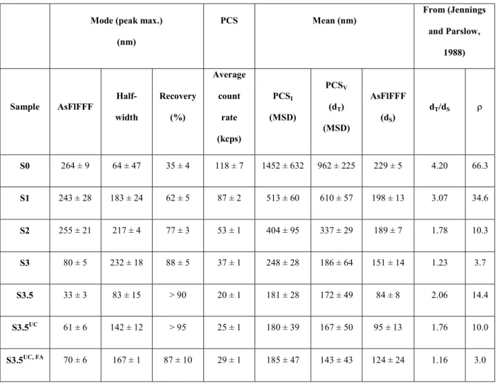
Table 3: Peak maxima and mean aggregate sizes of the dispersions obtained from AsFlFFF-/ICP-MS
395
measurements with the corresponding mean intensity (I)- and volume (V)-weighted sizes determined from
396
PCS analysis from the multimodal size distribution (MSD). The colloid recovery in the
AsFlFFF-397
measurements increases with decreasing sizes. dT/dS: equivalent spherical diameter (ESD) ratios, where dT
398
is the ESD for a translating disc-shaped particle determined by PCS (mean volume-weighted value, PCSV)
399
and dS is the equivalent Stokes’ spherical diameter for a sedimenting particle determined by AsFlFFF
400
(mean value); : calculated axial ratio, see section 3.1.4.2 for details.
401
Mode (peak max.) (nm) PCS Mean (nm) From (Jennings and Parslow, 1988) Sample AsFlFFF Half-width Recovery (%) Average count rate (kcps) PCSI (MSD) PCSV (dT) (MSD) AsFlFFF (dS) dT/dS S0 264 ± 9 64 ± 47 35 ± 4 118 ± 7 1452 ± 632 962 ± 225 229 ± 5 4.20 66.3 S1 243 ± 28 183 ± 24 62 ± 5 87 ± 2 513 ± 60 610 ± 57 198 ± 13 3.07 34.6 S2 255 ± 21 217 ± 4 77 ± 3 53 ± 1 404 ± 95 337 ± 29 189 ± 7 1.78 10.3 S3 80 ± 5 232 ± 18 88 ± 5 37 ± 1 248 ± 28 186 ± 64 151 ± 14 1.23 3.7 S3.5 33 ± 3 83 ± 15 > 90 20 ± 1 181 ± 28 172 ± 49 84 ± 8 2.06 14.4 S3.5UC 61 ± 6 142 ± 12 > 95 25 ± 1 180 ± 39 167 ± 50 95 ± 13 1.76 10.0 S3.5UC, FA 70 ± 6 167 ± 1 87 ± 10 29 ± 1 185 ± 47 143 ± 43 124 ± 24 1.16 3.0 402
The half-width values decrease only slightly for the dispersions S0 to S3.5 indicating that a
403
rather broad character of the size distributions remains. In addition, it should be noted that the
404
mean clay aggregate sizes obtained in the dispersions is higher than expected (Table 1),
405
especially for the dispersions where the smallest size is expected, i.e. in S3 and all S3.5
406
dispersions. This may be interpreted as an incomplete sedimentation during the centrifugation
21
due to the inaccurate assumption made considering a spherical shape of the particles in the
408
Stokes’ law calculation, since the particle shape is of high importance while included in
409
Stokes’ law (Kunkel, 1948).
410
The colloid recovery for each AsFlFFF-measurement (indicated in brackets in the legend in
411
Figure 3a and in Table 3, 4th column) can also help to understand the results. One explanation
412
for the low recoveries in S0 to S2 runs is the loss of particles in the AsFlFFF-channel due to
413
an irreversible attachment of notably larger sized aggregates to the membrane during the
414
fractionation process. The lower recovery of the Al-mass especially for the dispersions S0 and
415
S1 indicates the presence of large aggregates attaching to the accumulation wall in the
416
channel or moving too slowly to be detected under these conditions. This is in agreement with
417
the slow sedimentation process observed in the unstirred dispersions S0 and S1 over time
418
(Table 2). The recovery increases significantly with higher centrifugation forces, where higher
419
recoveries are reached for the dispersions obtained after the ultra-centrifugation step (S3.5 and
420 S3.5UC). 421 422 3.1.4.2 PCS 423
To complement the AsFlFFF analysis, the dispersions are monitored by PCS after dilution to
424
10 mg/L clay. The results of the PCS analyses are presented in Table 3. The table presents the
425
average count rates (in kilo counts per second (kcps)) which clearly decrease for
426
centrifugation steps with higher rotation rates, even though the colloid mass concentrations
427
are the same. Since the scattered intensity is highly dependent on the particle size, this is in
428
line with the size variations seen in the AsFlFFF-measurements (Table 3). The corresponding
429
values for the mean diameters of the clay aggregates are given, both as intensity-weighted
430
(PCSI) and as volume-weighted (PCSV) in Table 3 as obtained from the measurements by
22
considering the multimodal size distribution using the Non-Negatively constrained Least
432
Squares (NNLS) algorithm to fit the data (Bro and De Jong, 1997). The volume-weighted
433
diameter values (PCSV) are those which can be compared directly with the AsFlFFF data.
434
Looking into Table 3 (column 7 and 8), the results are comparable. The differences are
435
explained by losses of large particles in the AsFlFFF channel (especially for samples S0 and
436
S1) and by recalling that the PCS preferentially detect larger sized entities.
437
Nowadays, it is recognized that several techniques have to be used to combine the results
438
from particle size measurements and draw a more realistic description of a natural or synthetic
439
sample, containing particles of irregular shapes, especially clay nanoparticles (Beckett et al.,
440
1997; Bowen, 2002; Bowen et al., 2002; Cadene et al., 2005; Gallego-Urrea et al., 2014;
441
Gantenbein et al., 2011; Plaschke et al., 2001; Veghte and Freedman, 2014). More
442
information can be obtained from the AsFlFFF and PCS data following the development of
443
(Jennings and Parslow, 1988) extended by e.g. (Bowen et al., 2002), (Pabst and Berthold,
444
2007) and (Gantenbein et al., 2011). In brief, whatever equipment is used, the dimensions
445
obtained are equivalent sphere diameters (ESD) i.e. the diameters of spheres that would
446
behave the same as the particles in the sample, as a function of the method used. One should
447
have in mind that the ESD describes a 3-dimensional object with only one number. Flow FFF
448
provides a direct access to the Stokes’ diameter dS (Schimpf et al., 2000). “Particles under the
449
influence of Brownian agitation translate for all orientations and it is the random orientation
450
translation that is analysed in the PCS method” (Jennings and Parslow, 1988). Accordingly,
451
the PCS gives access to the equivalent diameter from frictional translatory diffusion data, dT.
452
Consequently, except for spherical particles, one cannot expect the derived ESD to be
453
identical from the two techniques as different physical phenomena are the basis of the
454
measurements. This is used presently as an advantage considering that no identical results
455
reveal the non-sphericity of the particles to be analysed and can thus serve to measure it. We
23
develop that possibility in the following discussion by comparing the ESD values (dS)
457
obtained with the AsFlFFF and the ESD values (dT) obtained with the PCS, i.e. the
volume-458
weighted ones from the MSD fitting.
459
According to Jennings (Jennings, 1993), a comparison between the ESD values from the
460
AsFlFFF (dS) and PCS (dT) gives access to the mean clay axial ratio (ρ) for the aggregates in
461
each dispersions defined as the aggregate surface diameter to thickness ratio for each
462
dispersions. In previous works (Jennings, 1993; Jennings and Parslow, 1988), Jennings
463
presents the mathematical expressions of the equivalent spherical diameter (ESD) according
464
to the analytical method used for its determination which are functions of the axial ratio. The
465
equations are given primarily for oblate and prolate spheroids with two limiting geometry
466
cases considered: the rod and the disc (to which the clay aggregate geometry may be
467
simplified). The ESD for a translating disc-shaped particle (dT) and the equivalent Stokes’
468
diameter (dS) for a sedimenting particle are expressed in equation (4) and (5) as (Jennings and
469 Parslow, 1988): 470 = ∙ Equation 4 471 = Equation 5 472
where = /t is the axial ratio of the disc-shaped particle, with being the surface diameter
473
of the disc-shaped particle and t its thickness.
474
Consequently, for a given particle, the ratio of these two ESD expressions may be used
475
inversely a posteriori to evaluate the axial or aspect ratio () of the particle and thus to obtain
476
the value of and t, if the clay aggregate is approximated by a disc of diameter and
477
thickness t. In the present work, the ratio dT/dS correspond to the ratio of the ESD determined
24
by AsFlFFF (dS) and PCS (dT) (volume-weighted mean value, PCSv). The calculated dT/dS
479
from the experimental mean diameters are presented in Table 3. The theoretical curve
480
d /d = f() obtained from Equation 4 and Equation 5 is plotted in Figure 4 and is used to
481
deduce the axial ratio () for each clay colloid dispersion reported in Table 3.
482
483
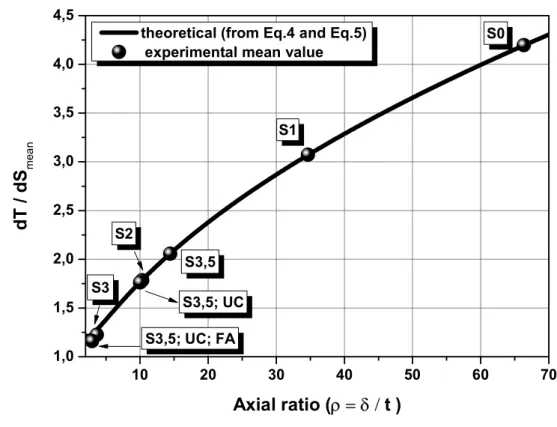
Figure 4: Theoretical dT/dS-ratio values calculated as a function of the axial ratio (black line) using
484
equations (4) and (5). The dT/dS-ratio values determined from the experimental mean PCS and AsFlFFF
485
ESD data are reported for each dispersion. A posteriori, the corresponding axial ratio is obtained and
486
presented in Table 3.
487
Obviously, > 1 for each dispersion as expected for clay aggregates having a disc-shaped
488
geometry. Interestingly, the -values are decreasing with increasing fractionation steps from
489
~35 (S1) down to ~3.7 (S3). (Note: due to the low AsFlFFF recovery, the -value obtained for
490 S0 (~66) is biased). 491 10 20 30 40 50 60 70 1,0 1,5 2,0 2,5 3,0 3,5 4,0 4,5 S3,5; UC; FA S3,5; UC S3 S2 S3,5 S1
theoretical (from Eq.4 and Eq.5) experimental mean value
d T / d S m ea n Axial ratio (t) S0
25
Once -values are known for each dispersion, one can back-calculate the corresponding mean
492
surface diameter, , and thickness, t, by using Equation 4 and Equation 5. The number of clay
493
layers is calculated by taking 1.3 nm as the thickness of one single clay mineral layer (basal
494
spacing) obtained by XRD results and according to (Meunier, 2005). The results are
495
summarized in Table 4. According to literature, the clay aggregates dimensions reported in
496
this work are plausible (Bergaya et al., 2006; Bouby et al., 2011; Hauser et al., 2002; Missana
497
et al., 2003; Plaschke et al., 2001; Schramm and Kwak, 1982a, b; Sposito, 1992; Tournassat et
498
al., 2011; Tournassat et al., 2003). The aspect ratio values determined agree with literature
499
data (Ali and Bandyopadhyay, 2013; Cadene et al., 2005; Gélinas and Vidal, 2010; Plaschke
500
et al., 2001; Tournassat et al., 2011; Tournassat et al., 2003; Weber et al., 2014; Veghte and
501
Freedman, 2014). Pictures obtained from SEM analysis of the dispersions S0 to S3 are
502
presented in the supporting file (see SIF-5). A raw evaluation of the AsFlFFF/MALLS data
503
according to (Baalousha et al., 2005; Baalousha et al., 2006; Kammer et al., 2005) allows to
504
compare the hydrodynamic (Rh) versus gyration (Rg) radius. The corresponding ratio (Rg/Rh),
505
called the shape factor, varies in the range [1.5-4] for the present measurements, and equals to
506
1 for a spherical particle. The shape factor increases as soon as the particles deviate from a
507
spherical shape, indicating that the montmorillonite aggregates are non-spherical.
508
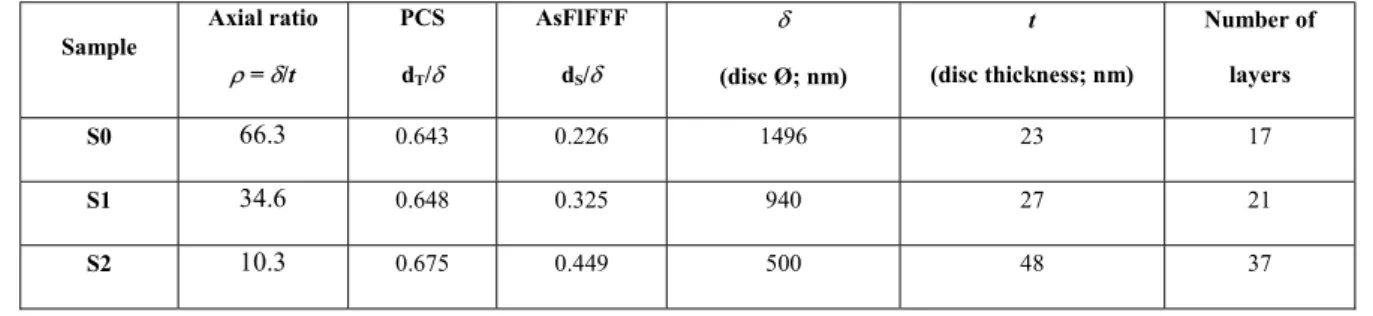
Table 4: Mean disc surface diameters () and number of layers calculated from PCS and AsFlFFF mean
509
equivalent sphere diameters (ESD) and the mathematical equations 4 and 5, according to (Jennings and
510
Parslow, 1988) for the clay aggregates. The number of layers is calculated by taking 1.3 nm as the
511
thickness, t, of one clay sheet, according to XRD results when considering one water layer.
512 Sample Axial ratio = /t PCS dT/ AsFlFFF dS/ (disc Ø; nm) t (disc thickness; nm) Number of layers S0 66.3 0.643 0.226 1496 23 17 S1 34.6 0.648 0.325 940 27 21 S2 10.3 0.675 0.449 500 48 37
26 S3 3.7 0.743 0.546 250 68 52 S3.5 14.4 0.664 0.303 258 18 14 S3.5UC 10.0 0.676 0.385 246 25 19 S3.5UC,FA 3.0 0.767 0.546 187 63 48 513
By plotting the oblate spheroid ESD as a function of the axial ratio (Jennings and Parslow,
514
1988), the ESD is found to always be smaller than the true dimension, . This is true for both
515
measurement techniques used in this study as well (Table 4). From S0 to S3, there is a clear
516
trend in decreasing surface diameter, and increasing thickness, t. Nevertheless, the AsFlFFF
517
results are obtained from measurements with rather low recoveries while the PCS is detecting
518
all aggregates in the dispersion. Consequently, the results presented in Table 4 can only be
519
considered as partly representative of the complete samples due to the low recoveries in the
520
AsFlFFF-measurements. If one considers the dispersions where ≥ 50% of the mass is
521
recovered (S1 and smaller), the mean disc surface diameter () of the clay aggregates is
522
decreasing, whereas the thickness (t) is increasing with further fractionation steps. The
523
difference between the dispersion S3 and S3.5 appears only in the thickness of the clay
524
aggregates. As expected, comparable results are obtained for the dispersions S3.5 (obtained
525
after continuous (ultra-)centrifugation steps) and S3.5UC (obtained after one single
ultra-526
centrifugation step). Interestingly, the thickness, and thus number of clay sheets, appears
527
slightly higher in presence of FA during the fractionation, which may indicate that the
528
presence of FA could stabilize thicker clay aggregates, i.e. maintain a larger number of
529
stacked clay mineral layers together.
530
In conclusion, the fractionation protocol developed in the present study enables to obtain
531
heterogeneous dispersions of clay aggregates. Assimilating the clay aggregates to discs of
532
surface diameter and thickness t, the results indicate presence of aggregates with mean
27
surface diameters ranging from ~245 nm up to 1500 nm and with mean thicknesses ranging
534
from ~18 up to 70 nm (~14 to 52 clay layers). In presence of FA during the fractionation, clay
535
aggregates with a surface diameter of ~190 nm can be isolated, but with a slightly larger
536
thickness (~63 nm) as those obtained under the same fractionation conditions in absence of
537
FA. The present results would greatly benefit of complementary investigations involving the
538
use of other microscopy techniques like AFM.
539
3.1.5 An attempt to estimate the mean number of edge sites
540
By approximating clay aggregates to discs of mean diameter , estimations of the mean
541
number of edge sites in each clay dispersion were performed. This will be used in an attempt
542
for better interpretation of the data for radionuclides sorption by surface complexation and
543
sorption reversibility (manuscripts in preparation).
544
Estimations of the number of edge sites are performed according to the work of White and
545
Zelazny (White and Zelazny, 1988) and Tournassat et al. (Tournassat et al., 2003), assuming a
546
clay density of 2.7 g/cm³, and are presented in Table 5. It is considered that the stacking of
547
clay mineral layers does not change the accessibility to the lateral surfaces, only the interlayer
548
basal surfaces are not accessible.
549
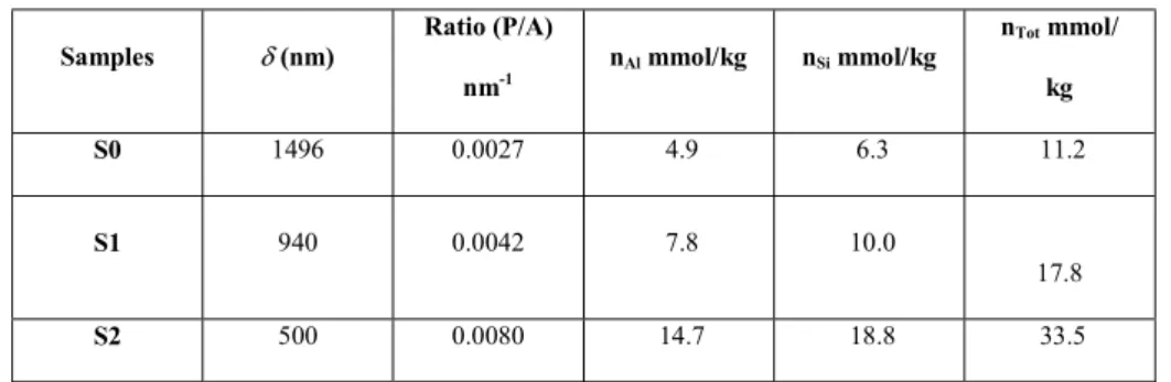
Table 5: Estimation of the mean number of edge sites for each clay dispersion from PCS- and
AsFlFFF-550
data. The perimeter of a clay stack is noted as P and is calculated by using the clay aggregate disc
551
diameter . The clay disc area (A) is calculated by using as the mean diameter of the clay aggregate as
552
well. .
553
Samples (nm) Ratio (P/A)
nm-1 nAl mmol/kg nSi mmol/kg
nTot mmol/ kg S0 1496 0.0027 4.9 6.3 11.2 S1 940 0.0042 7.8 10.0 17.8 S2 500 0.0080 14.7 18.8 33.5
28 S3 250 0.0161 29.4 37.6 67.0 S3.5 258 0.0152 28.4 36.3 64.7 S3.5UC 246 0.0162 29.8 38.1 67.9 S3.5UC,FA 187 0.0214 39.3 50.2 89.5 554
The results show variations up to a factor ~8, but they are only considered as approximations
555
since the aggregate dimensions are underestimated. Taking a regular disc to mimic smectite
556
aggregates does not take into account their convexities and concavities which lead to an
557
increase in their surface area and perimeter. When considering the dispersions with the
558
smaller mean clay size (S3.5, S3.5UC and S3.5UC,FA), the results are in agreement with those of
559
Tournassat et al. (Tournassat et al., 2003).
560
3.2 Stability studies
561
Evaluation of the Al-AsFlFFF/ICP-MS fractograms for the montmorillonite fractions reveals
562
broad clay aggregate size distributions that might be constituted by several different clay size
563
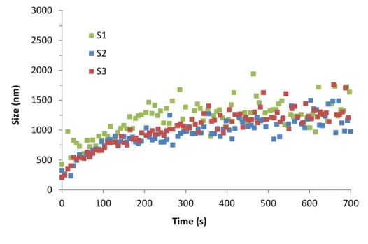
fractions (Figure 3). Consequently, it is not surprising that the data obtained from the stability
564
studies are very scattered (Figure 5). Therefore, it becomes challenging to clearly observe the
565
increase in mean particle size which reflects the agglomeration rate (especially for the
566
dispersion S0 which will not be further considered). In addition, one has to consider that the
567
agglomeration behavior of smaller sized particles are probably hidden by the dominant
568
scattered light intensities from larger particles as the PCS preferentially detect those larger
569
sized entities. Nevertheless, the results from the data evaluation are less scattered for the
570
dispersions obtained after several centrifugation steps (S3 and S3.5).
29 572
Figure 5: Increase in hydrodynamic diameter for three of the montmorillonite dispersions while adding
573
0.01 M CaCl2 to the dispersions at pH 7.
574
575
The calculated stability ratios (W) for all dispersions at pH 7 and for different ionic strengths
576
are presented in Figure 6. The presented W-values are obtained for an ionic strength set by
577
addition of the electrolytes NaCl, CaCl2 or MgCl2. As expected, W decreases with increasing
578
ionic strength. This is clearly seen after addition of NaCl (Figure 6a) and is consistent with
579
the DLVO-theory. Furthermore, addition of CaCl2 and MgCl2 affects the montmorillonite
580
particles more strongly than addition of the same ionic strength set by NaCl since the lowest
581
concentrations of CaCl2 and MgCl2 are already enough to destabilize the montmorillonite
582
particles (Figure 6b and 6c), as expected from previous studies (Schudel et al., 1997). This is
583
in line with the well-known Shulze-Hardy rule (Overbeek, 1980). The decrease in stability
584
ratio in presence of divalent cations is partly explained by specific interaction of divalent
585
cations as previously reported in the literature (French et al., 2009; Keiding and Nielsen,
586
1997; Norrfors, 2015; Oncsik et al., 2014; Pantina and Furst, 2006).
587 0 500 1000 1500 2000 2500 3000 0 100 200 300 400 500 600 700 Si ze (n m ) Time (s) S1 S2 S3
30
According to the DVLO-theory, considering the interaction between two identical spherical
588
particles, the calculated Van der Waals (VdW)-forces increase for increasing particle size
589
(Ottewill and Shaw, 1966; Reerink and Overbeek, 1954; Shah et al., 2002). However, it has
590
been found previously that in a system of high ionic strength, i.e. where no electrostatic
591
repulsions are present, the kinetic energy dominates over the VdW-forces and the
592
agglomeration rate constants of spherical latex particles are therefore independent of the
593
particle size (Norrfors, 2015). Even though clay aggregates are known to have different
594
shapes and compositions than the latex particles present in the previous study (Norrfors,
595
2015), the domination of the kinetic energy can be one explanation of the absence of
596
significant differences between the colloidal dispersions in this study (Figure 6). The absence
597
of particle size dependency on the stability ratios is further in agreement with previous studies
598
(Behrens et al., 2000; Ottewill and Shaw, 1966) but once again, one should have in mind that
599
PCS measurements in polydisperse dispersions favour larger sized particles and thereby
600
hiding the agglomeration behaviour of the smaller sized ones. Previous studies of
601
polydisperse dispersions (Chang and Wang, 2004; Jia and Iwata, 2010) indicate that their
602
stability ratio is smaller than for a mono disperse system, which may be seen in this study.
31 604
605
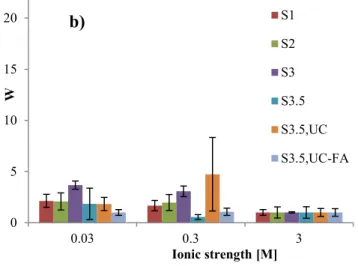
606
Figure 6: Stability ratios for the colloidal dispersions after addition of a) NaCl b) CaCl2 or c) MgCl2, at pH
607
7. Infinity is set to 20 in the figures.
608
609
Finally, no significant differences in stability are observed in presence or absence of FA in the
610
dispersions. Previous studies present a stabilization of the clay particles in presence of FA
611
(Kretzschmar et al., 1998) and notice that the stabilization properties of FA decreases with
612
increasing pH, due to the lower FA adsorption to clay surfaces. In the present study of
613
agglomeration, coursed by addition of CaCl2, the relative high concentration of divalent ions,
614 0 5 10 15 20 25 0.01 0.1 1 3 W Ionic strength [M] S1 S2 S3 S3.5 S3.5,UC S3.5,UC-FA a) 0 5 10 15 20 0.03 0.3 3 W Ionic strength [M] S1 S2 S3 S3.5 S3.5,UC S3.5,UC-FA b) 0 5 10 15 20 0.03 0.3 3 W Ionic strength [M] c) S1 S2 S3 S3.5 S3.5,UC S3.5,UC-FA
32
Ca2+, induced agglomeration with the same agglomeration rate in both presence and absence
615
of FA.
616
4 Conclusions
617
A protocol to obtain montmorillonite colloid dispersions with different size fractions
618
is developed in this study. It is based on a sedimentation step followed by sequential
619
or direct (ultra-)centrifugation.
620
Montmorillonite aggregates of same composition are proved to be present in the
621
different dispersions as concluded from both the chemical analysis and the XRD
622
results. Calcium is associated to the clay particles as natural calcite or due to the fast
623
ionic exchange processes arising under the present experimental conditions. An instant
624
release of sodium and sulfate occurs when the bentonite is suspended in the SGW.
625
This is explained by dissolution of gypsum or/and celestite naturally present in the
626
unpurified MX-80 bentonite.
627
Mean equivalent sphere diameters (EDS) values obtained by different methods agree
628
when normalized to comparable physical properties, leading to a mean hydrodynamic
629
size of the clay aggregates from ~960 nm down to ~ 85 nm. Nevertheless, after
630
applying mathematical treatments, the differences recorded in the initial data between
631
the AsFlFFF (giving the Stokes’ diameter) and the PCS (giving a frictional translatory
632
diffusion diameter) are used to estimate the mean diameter and the thickness t of the
633
clay aggregates in the different dispersions after approximating those to regular
disc-634
shaped aggregates consisting of stacked clay mineral layers. According to our
635
calculation, varies from 1.5 µm down to ~190 nm and t lies in the range of 18 to 70
636
nm. The number of sheets (clay mineral layers) is determined by dividing the
637
thickness t by 1.3 nm (thickness of one single clay layer in basal spacing). The