Modelling photochemistry in alpine valleys

HAL Id: hal-00328401

https://hal.archives-ouvertes.fr/hal-00328401

Submitted on 12 Sep 2005

HAL is a multi-disciplinary open access

archive for the deposit and dissemination of

sci-entific research documents, whether they are

pub-lished or not. The documents may come from

teaching and research institutions in France or

abroad, or from public or private research centers.

L’archive ouverte pluridisciplinaire HAL, est

destinée au dépôt et à la diffusion de documents

scientifiques de niveau recherche, publiés ou non,

émanant des établissements d’enseignement et de

recherche français ou étrangers, des laboratoires

publics ou privés.

Modelling photochemistry in alpine valleys

G. Brulfert, C. Chemel, E. Chaxel, J. P. Chollet

To cite this version:

G. Brulfert, C. Chemel, E. Chaxel, J. P. Chollet. Modelling photochemistry in alpine valleys.

Atmo-spheric Chemistry and Physics, European Geosciences Union, 2005, 5 (9), pp.2355. �hal-00328401�

European Geosciences Union

and Physics

Modelling photochemistry in alpine valleys

G. Brulfert, C. Chemel, E. Chaxel, and J. P. Chollet

Laboratory of Geophysical and industrial Fluid Flows (University J. Fourier, INP Grenoble, CNRS), BP53, 38 041 Grenoble cedex, France

Received: 1 July 2004 – Published in Atmos. Chem. Phys. Discuss.: 21 March 2005 Revised: 19 July 2005 – Accepted: 11 August 2005 – Published: 12 September 2005

Abstract. Road traffic is a serious problem in the Chamonix Valley, France: traffic, noise and above all air pollution worry the inhabitants. The big fire in the Mont-Blanc tunnel made it possible, in the framework of the POVA project (POllution in Alpine Valleys), to undertake measurement campaigns with and without heavy-vehicle traffic through the Chamonix and Maurienne valleys, towards Italy (before and after the tun-nel re-opening). Modelling is one of the aspects of POVA and should make it possible to explain the processes leading to episodes of atmospheric pollution, both in summer and in winter. Atmospheric prediction model ARPS 4.5.2 (Ad-vanced Regional Prediction System), developed at the CAPS (Center for Analysis and Prediction of Storms) of the Univer-sity of Oklahoma, enables to resolve the dynamics above a complex terrain. This model is coupled to the TAPOM 1.5.2 atmospheric chemistry (Transport and Air POllution Model) code developed at the Air and Soil Pollution Laboratory of the Ecole Polytechnique F´ed´erale de Lausanne. The numer-ical codes MM5 and CHIMERE are used to compute large scale boundary forcing.

This paper focuses on modelling Chamonix valley using 300-m grid cells to calculate the dynamics and the reactive chemistry which makes possible to accurately represent the dynamics in the Chamonix valley (slope and valley winds) and to process chemistry at fine scale. The summer 2003 in-tensive campaign was used to validate the model and to study

chemistry. NOyaccording to O3reduction demonstrates a

VOC controlled regime, different from the NOx controlled

regime expected and observed in the nearby city of Greno-ble.

Correspondence to: G. Brulfert

([email protected])

1 Introduction

Alpine valleys are sensitive to air pollution due to emission sources (traffic, industries, individual heating), morphology (narrow valley surrounded by high ridge), and local meteo-rology (temperature inversions and slope winds). Such situa-tions are rarely investigated with specific research programs taking into account detailed gas atmospheric chemistry. Sev-eral studies of the influence of atmospheric dynamics over complex terrain on air quality took place with field cam-paigns in the Alpine area over the last two decades. The pro-gram TRANSALP (a component of EUROTRAC-TRACT) included several field campaigns, with, among others, (i) an intensive sampling campaign with high density network for

ozone measurements on a 300×300 km2area (L¨offler-Mang

et al., 1998), (ii) an intensive sampling campaign with the follow up of the dispersion of a passive tracer released in the Rhine valley (which is about 40 km width on average) (Am-brosseti et al., 1998). The POLLUMET program (Lehning et al., 1996) focused on processes controlling oxidant con-centrations in the Swiss Plateau. These two programs mostly dwelt with meso scale processes, and did not take into ac-count in detail atmospheric dynamics in narrow valleys. In the same way, one of the objectives of the MAP program (http://www.map.meteoswiss.ch) was devoted to the study of the evolution of the planetary boundary layer in complex ter-rain at the meso scale, but no measurements were conducted

in parallel on any aspect of atmospheric chemistry. The

programs VOTALP I (Wotawa and Kromp-Kolb, 2000) and VOTALP II (http://www.boku.ac.at/imp/votalp/votalpII.pdf) were essentially devoted to the study of ozone production and vertical transport over the Alps. The modelling in this pro-gram (Grell et al., 2000), coupling a non hydrostatic model with a photochemistry model at a resolution of 1×1 km for the inner domain, showed, among other, the influence of the valley wind in the advection of chemical species from the foreland to the inner valley. The authors conclude that the

2342 G. Brulfert et al.: Modelling photochemistry in alpine valleys evaluation of the pollutant budget in the valley requires a

finer grid as well as a detailed emission inventory. Couach et al. (2003) present a modelling study coupling atmospheric dynamics and photochemistry (at a 2×2 km scale) in the case of the Grenoble (France) area, which is a large glacial val-ley in the French Alps. This study is connected to a 3-day field campaign conducted in summer 1999, including a large array of ground and 3-D measurements dedicated to ozone and its precursors. Again, this study showed the large in-fluence of the valley wind on the distribution of ozone con-centrations. The modelled ozone concentrations were in rea-sonable agreement with 3-D measurements. Finally, the Air Espace Mont Blanc study (Espace Mont Blanc, 2003) was conducted by the Air Quality networks in France, Italy, and Switzerland. The field study was based on a 1 year moni-toring (June 2000–May 2001) at stations around the “Massif

du Mont Blanc”, for regulated species (SO2, NOx, O3, PM10

and PM2.5).

These previous studies underlined the limitations of the models in handling detailed atmospheric dynamics in com-plex terrain when using only 1×1 km resolution, while these processes are the dominant factors controlling the concentra-tions fields.

Following the accident under the Mont Blanc tunnel (Fig. 1) on 24 March 1999, international traffic between France and Italy was stopped through the Chamonix valley (France). The heavy-duty traffic (about 2130 trucks per day) has been diverted to the Maurienne Valley, with up to 4250 trucks per day. The campaigns were scheduled both before and after the reopening of the tunnel in order to directly in-vestigate the impact of international heavy duty traffic on air quality. However, the reopening of the tunnel was staged in different phases from March 2002 (for personal vehicles only) until March 2003 (open to all vehicles without restric-tion). International traffic through the tunnel during the last two intensive observation periods of observations (IOP) had not returned to the level of the period before the accident, with only about 1840 personal vehicles and 590 trucks/day on average during the winter 2003 IOP and about 4180 per-sonal vehicles and 910 trucks/day on average during the sum-mer 2003 IOP.

The general topics of the POVA program (launched in 2000) are the comparative studies of air quality and the mod-elling of atmospheric emissions and transport in these two French alpine valleys before and after the reopening of the tunnel to heavy duty traffic to identify the sources and char-acterize the dispersion of pollutants. The program includes several field campaigns, associated with 3-D modelling in order to study impact of traffic and local development sce-narios.

Firstly the area of interest and numerical models in use are presented together with methods to prescribe boundary con-ditions. Main features of the emission inventory are given. After a validation from comparison with field experiments for dynamic and chemistry, computations of photochemical

indicators during a summer IPO conclude to a VOC sensitive regime.

2 The area of interest

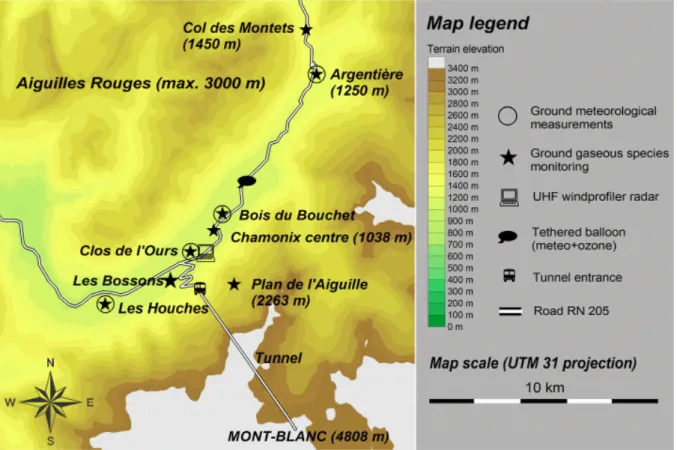
The Chamonix valley is 23 km long, closed in its lower end by a narrow defile (the Cluse pass) and at the upper side by the Col des Montets (1464 m a.s.l.) leading to Switzerland (Fig. 1). The general orientation of the valley is globally

NE-SW. With North latitude of 45.92◦ _{and East longitude}

of 6.87◦_{, the centre of the area is at approximately 200 km}

from Lyon (France), 80 km from Gen`eve (Switzerland) and 100 km from Torino (Italy). The valley is rather narrow (1 to 2 km on average on the bottom part) and 5 km from ridge to ridge, with the valley floor at 1000 m a.s.l. on average, surrounded by mountains culminating with the Mont Blanc peak (4810 m a.s.l.). Vegetation is relatively dense with many grassland and forest areas (Fig. 2).

There are no industries or waste incinerators in the valley, and the main anthropogenic sources of emissions are vehicle traffic, residential heating (mostly with fuel and wood burn-ing), and some agricultural activities. The resident popula-tion is about 12 000 but tourism brings in many people (on average 100 000 person/day in summer, and about 5 millions overnight stays per year), mainly for short term visits. There is only one main road supporting all of the traffic in and out of the valley, but secondary roads spread over all of the val-ley floor and on the lower slopes. During the closing of the Mont-Blanc tunnel leading to Italy, the traffic at the entrance of the valley (14 400 vehicles/day on average) was mostly composed of cars (91% of the total, including 50% diesel powered), with a low contribution of local trucks (5%) and of buses for tourism (1%). Natural sources of emissions are limited to the forested areas, with mainly coniferous species (95% of spruce, larch and fir).

3 Model for simulation

Because of the orography, slope winds are observed. Their thickness is around 50 to 200 m and depends on local orog-raphy effects. Horizontal resolution must be under 1 km to describe correctly meteorological and chemistry processes. A terrain following coordinate is appropriate to the vertical resolution. Non-hydrostatic models have to be used at meso-scale. The influence of regional meteorology and ozone con-centration is important, overlapping models give boundary conditions.

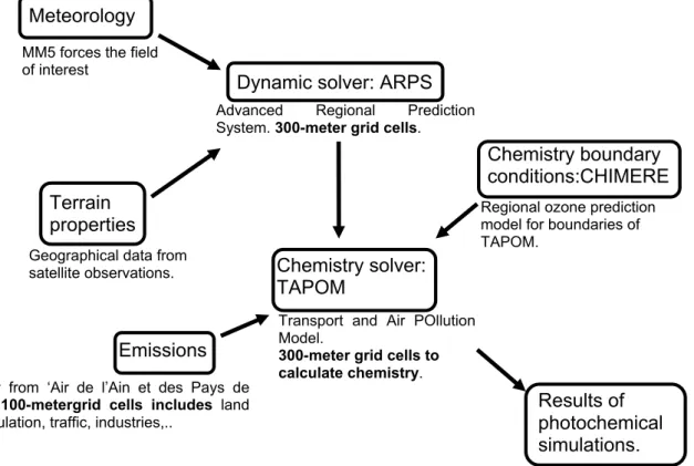
To sum up, the modelling system for the valley itself is made of the meso-scale atmosphere model ARPS 4.5.2 and the troposphere chemistry model TAPOM 1.5.2.

Fig. 1. Topography of Chamonix valley: main measurement sites (centre of the valley: Latitude 45.92◦N, longitude 6.87◦E). Road is the white line.

Table 1. Hierarchy of computational domains.

Typical extend Grid nodes Grid size Code in use Code in use nx E-W×ny N-S 1x=1y (km) for dynamics for chemistry

Domain 1 France 1500 km 45×51 27 MM5 CHIMERE

Domain 2 Southeastern France 650 km 69×63 9 MM5 CHIMERE

Domain 3 Savoie mountains 350 km 96×96 3 MM5

Domain 4 Haute-Savoie Dept. 50 km 67×71 1 ARPS TAPOM

Domain 5 Chamonix valley 25 km 93×103 0.3 ARPS TAPOM

4 Model for atmosphere dynamics

Large eddy simulation was used to study meso-scale flow fields in both valleys. The numerical simulations presented here have been conducted with the Advanced Regional Pre-diction System (ARPS), version 4.5.2 (Xue et al., 2000, 2001). Lateral boundary conditions were externally-forced from the output of larger-scale simulations performed with the Fifth-Generation Penn State/NCAR Mesoscale Model

(MM5) version 3 (Grell et al., 1995). MM5 is a

non-hydrostatic code which allows meteorological calculation at

various scales with a two-way nesting technique. In the

present study three different domains were used with MM5

(Table 1). ARPS is used at finer grids because MM5 was ob-served not to be accurate enough at resolution less than 1 km (Chaxel et al., 2004). For the Chamonix valley modelling with ARPS, two grid nesting levels were used as shown in Table 1. A geographical description of domains is available in Fig. 3.

4.1 Model for atmosphere chemistry

ARPS is coupled off-line with the TAPOM 1.5.2 code of at-mospheric chemistry (Transport and Air POllution Model) developed at the LPAS of the EPFLausanne (Clappier, 1998;

2344 G. Brulfert et al.: Modelling photochemistry in alpine valleys

Fig. 2. Landuse of Chamonix valley in summer. Red is infrastructure, yellow is grassland, dark green is forest, pale green is high altitude

vegetation, white-grey is rock and snow, the dark line is the main road.

Fig. 3. Geographical description of MM5 (D1, D2, D3) domains over Europe and ARPS (D4, D5) domains over Haute-Savoie department.

Chemistry solver:

TAPOM

Emissions

Dynamic solver: ARPS

Meteorology

Terrain

properties

Results of

photochemical

simulations.

Advanced Regional Prediction System. 300-meter grid cells.

Transport and Air POllution Model.

300-meter grid cells to calculate chemistry.

Geographical data from satellite observations.

Inventory from ‘Air de l’Ain et des Pays de Savoie’. 100-metergrid cells includes land use, population, traffic, industries,..

Chemistry boundary

conditions:CHIMERE

Regional ozone prediction model for boundaries of TAPOM.

MM5 forces the field of interest

Fig. 4. Description of the modelling system for photochemical simulations.

dynamics and reactive chemistry make possible to accurately represent dynamics in the valley (slope winds) (Anquetin et al., 1999) and to process chemistry at fine scale.

TAPOM is a three dimensional eulerian model with ter-rain following mesh using the finite volume discretisation. It includes modules for transport, gaseous and aerosols chem-istry, dry deposition and solar radiation. It takes into ac-count the extinction of solar radiation by gases and aerosols in the gaseous chemistry calculation. Chemistry and pol-lutant transport are not expected to significantly change at-mosphere radiative properties. Hence chemistry is consid-ered not to modify dynamics which allows off-line coupling: meteorological data computed from ARPS are passed on to TAPOM every 20 min with linearly interpolating data in be-tween. A full description of the ARPS-TAPOM coupling is given in Brulfert (2004). TAPOM uses the Regional At-mospheric Chemistry Modelling (RACM) scheme

(Stock-well et al., 1997). RACM is a completely revised

ver-sion of RADM2. The mechanism includes 17 stable

in-organic species, four inin-organic intermediates, 32 stable or-ganic species (four of these are primarily of biogenic

ori-gin) and 24 organic intermediates, in 237 reactions. In

RACM, the VOCs are aggregated into 16 anthropogenic and three biogenic model species. The grouping of chemical or-ganic species into the RACM model species is based on the magnitudes of the emissions rates, similarities in functional

groups and the compound’s reactivity toward OH (Middleton et al., 1990). RACM was compared with other

photochem-ical mechanisms and it gives very good results for O3 with

regards to the percentage of deviation of individual mecha-nisms from average values (Jimenez et al., 2003).

For the boundary conditions, CHIMERE, a regional ozone prediction model, from the Institut Pierre Simon Laplace, gives concentrations of chemical species at five altitude lev-els (Schmidt et al., 2001) using its recent multi-scale nested version.. Then, CHIMERE is used at a space resolution of 27 km and 6 km to give chemical species initialisation and boundaries. Chemical concentrations calculated on a large scale domain are used at the boundaries of a smaller one. Then, we can have a very good description of the temporal variation of the background concentrations of ozone and of other secondary species. It is possible to use CHIMERE data for TAPOM because the chemical mechanism (respectively MELCHIOR and RACM) are close on to the other.

The whole methodology of modelling system to obtain photochemical simulations is described in Fig. 4.

5 Emission inventory

The emission inventory is based on the CORINAIR methodology and SNAPS’s codes, with a 100×100 m grid and includes information (land use, population, traffic,

2346 G. Brulfert et al.: Modelling photochemistry in alpine valleys

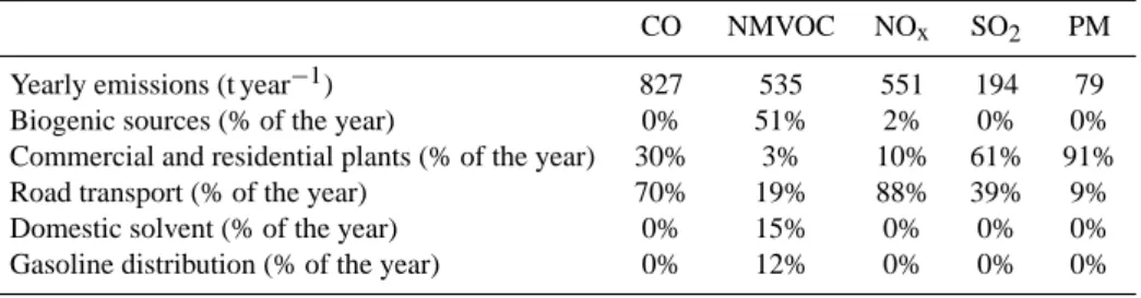
Table 2. Emission inventory for 1998 in the area of interest (t year−1).

CO NMVOC NOx SO2 PM

Yearly emissions (t year−1) 827 535 551 194 79 Biogenic sources (% of the year) 0% 51% 2% 0% 0% Commercial and residential plants (% of the year) 30% 3% 10% 61% 91% Road transport (% of the year) 70% 19% 88% 39% 9% Domestic solvent (% of the year) 0% 15% 0% 0% 0% Gasoline distribution (% of the year) 0% 12% 0% 0% 0%

Table 3. Classes of the emission inventory.

Traffic sources Anthropogenic Biogenic

sources sources

Heavy vehicles Commercial boiler Forest Utilitarian vehicles on motorway Residential boiler Grassland Utilitarian vehicles on road Domestic solvent

Cars Gas station Cars in city

Aerial traffic

industries...) gathered from administrations and field

investi-gations. The area covers 695 km2. The emission inventory is

space and time-resolved and includes the emissions of NOx,

CO, CH4, SO2and non methane volatile organic compounds

(NMVOC). As expected, the result which includes both bio-genic and anthropobio-genic sources, shows large emissions of pollutants due mainly to the presence of road transport and plants (Table 2).

These emissions are lumped into 19 classes of VOC as re-quired by the Regional Atmospheric Chemistry Mechanism (RACM) (Stockwell et al., 1997).

Emission classes are given in the Table 3. The emission inventory takes into account roads and access ramps to the tunnel adjusting emissions to the slope of the road. A spe-cific feature of emission is the significant contribution of heavy vehicles (>32 tons). The emissions are distributed at the hourly level by taking account of the season and the day of the week. Further details on this emission inventory are given (Brulfert et al., 2005).

6 Validation

The simulations presented here take a full account of the real meteorology of the week of computation during the summer POVA IPO (5 July 2003 to 11 July 2003).

6.1 High-resolution meteorological simulation:

compari-son with surface and wind profiler data

The redistribution of pollutants and therefore the ozone pro-duction is very dependent on meteorological conditions. The observed meteorological situation during the 7 days of inten-sive period of observation (IPO) is summarized in Table 4. A north westerly wind with sun prevailed. In this complex mountainous area, wind balance and slope winds are impor-tant for the transport of chemical species.

To validate the simulated meteorological fields, we com-pare the model results to surface observations (Fig. 5). Temperature at sites “Les Houches”, “Chamonix” and “Ar-genti`ere” shows reasonable agreement for the minimum and maximum, respectively at 01:00 and 13:00 TU. A slight dis-crepancy at minimal value may be attributed to the difficul-ties in accurately modelling cooling of lower layer and hu-midity content of soil canopy at night. One of the difficulties was to parameter the humidity and the soil temperature with-out measurements. Furthermore, the real soil of these valleys is heterogeneously distributed in small parcels strongly dif-fering one from the other: grassland, rocks, forests, ice.

Results in Fig. 5 are given from the very beginning of the computation, significant discrepancies on the first day are then to be attributed to the spin-up from initial conditions. Discrepancies on 9 July are due to a stormy day (Table 4) since ARPS was run in fine weather conditions without acti-vating nebulosity and detailed micro physics. Maxima values of temperature are often overestimated partly due to inaccu-racies in detailed soil description, partly because of the shift from computed value at the centre of the first mesh to ground level.

Wind force at site “Clos de l’ours” corresponds to mea-surement with maximum at 13:00 TU, nocturnal cycle is present. The computed wind velocity at the station “Bois du Bouchet” is more important than the real velocity because of a local effect with this station: trees are very close and slow down wind at ground level especially when flowing down valley.

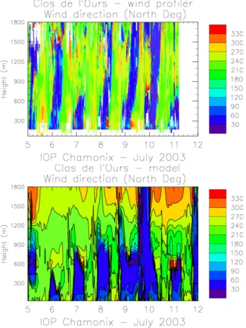
Shifts in wind direction occur at the right times at sites “Bois du Bouchet”, “Argenti`ere” and “Clos de l’ours” at 08:00 and 20:00 TU. Discrepancies in wind direction at the

2348 G. Brulfert et al.: Modelling photochemistry in alpine valleys

Table 4. IOP 2003 meteorology from 5 July to 11 July.

19

at 4500 m asl 2.5 m/s NW 4 m/s NW 4 m/s W (<1m/s)Not significant (<1m/s)Not significant N to NW 5.5 m/s 7 m/s NW

Table 4. IOP 2003 meteorology from July 5 to July 11.

Fig. 6a. Wind force from the wind profiler (top) compared to results

(bottom) from the computation.

beginning and end of each shift in Fig. 5 are non significant since corresponding to weak and therefore inaccurately mea-sured wind.

Profiler data are in good agreement with values from the model (Figs. 6a and b): wind reversal starts and stops at the same time. The altitude of the synoptic wind is well repre-sented. Model results taken into account come from the first layer above the topography. ARPS works with a terrain

fol-Fig. 6b. Wind direction from the wind profiler (top) compared to

results from the computation (bottom).

lowing coordinate. As above mentioned, wind direction has

not to be considered for weak (e.g. less than 1 m s−1) wind.

The boundary layer thickness can be estimated from wind profiler data. It is well simulated all along the day, except on 9 July because of stormy instable weather. Further discussion about measurements and layer thickness assessment is given

in (Chemel and Chollet., 20051).

1_{Chemel, C., Chollet, J. P.: Observations of the daytime}

at-mospheric boundary layer in deep alpine valleys,Boundary-Layer

fields are very realistic: temperature does not show signif-icant bias. The evolution of the thickness of the inversion layer is well simulated. Wind direction and forces are well reproduced with wind reversal observed at the same times in the model and from measurements. Therefore, meteorologi-cal fields may be viewed as realistic enough to drive transport and mixing of chemical species.

6.2 High-resolution chemistry simulation: comparison

with surface data

Concentrations of pollutants in the valley (such as O3 or

NO2) are rather low at least when compared with large cities:

values peak at 75 ppb for O3and 40 ppb for NO2compared to

100 ppb for O3and 50 ppb for NO2in nearby city of Lyon or

Grenoble. To validate the simulated chemical fields, model results and surface observations are compared during the summer 2003 IPO. Model results taken into account come from the first layer above the topography. TAPOM works with a terrain following coordinate.

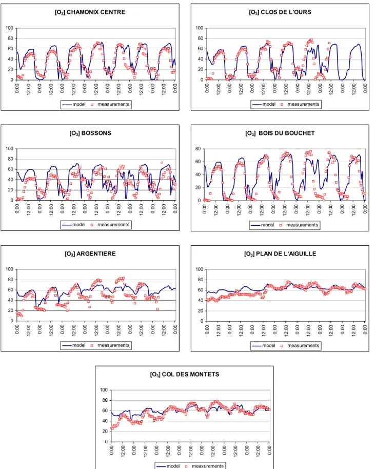
Ozone from the observation and from the model is in good agreement in both urban and rural stations (Fig. 7). Both spatial and temporal variability of the simulated ozone con-centrations correspond reasonably well to the measured val-ues. Figure 9 shows the correlations between the measured and simulated ozone concentrations for all the IPO days ex-cept for the stormy day (9 July, 2003). Values of correlation

coefficients are significantly high with 0.73<R2<0.76. The

correlation coefficient R between results from the model (f) and measurements (r) is defined as:

R = 1 N N P n=1 (fn−f )(rn−r) σfσr , (1)

where f and r are the mean values and σf and σr are the

standard deviations of f and r, respectively.

These results can be compared to the same correlations

in Grenoble during a high ozone episode with R2=0.64 for

urban station and R2=0.42 for suburban stations (Couach et

al., 2004).

The model significantly underestimates O3at night in “Les

Bossons”. It may be attributed to the proximity of the mo-torway (120 m) and the tunnel entrance (240 m). Because

of poor mixing at night, NOxmay be overestimated by the

model. The overestimation observed at station “Argenti`ere”

is due to NOx emissions which are presumably

underesti-mated in this rural part of the valley because of a lack of any local traffic record.

Background stations (“Col des Montets” and “Plan de l’aiguille”) are directly under regional influence. The ampli-tude of the variation of ozone concentrations are low, it does not make sense to give correlation coefficient. The relative

Meteorology, in review, 2005.

the stormy day) is 14% at the site “Plan de l’aiguille” and 6% for the site “Col des Montets” (respectively 12 and 3% without the first day spin up).

It is possible to observe a more important effect of lo-cal sources in the south part of the valley: amplitude of ozone concentration is more important for “Chamonix cen-tre”, “Clos de l’ours”, “Bossons” and “Bois du Bouchet”. There is a titration of ozone by NO emissions. In the north part of the valley, amplitude of concentration is less impor-tant, with values of background at site “Argenti`ere” and “Col des Montets”. Road traffic is less important there.

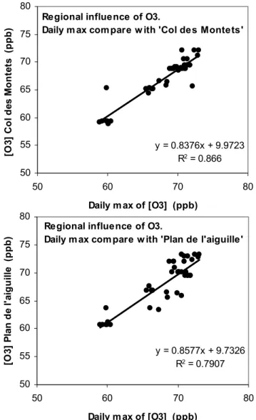
The influence of regional ozone in the valley is prepon-derant. If we correlate daily maximum of ozone concentra-tion at every site with the concentraconcentra-tion of background sta-tions at the same hour, high values of coefficients of

corre-lation are obtained (R2=0.87 for “Col des Montets” station

and R2=0.79 for “Plan de l’aiguille” station) as shown with

Fig. 10.

Ratio of regional O3concentration to urban stations daily

maximum (at the hour of the maximum) gives important

information about regional influence of O3. High values

(≈1) are associated with regional preponderance and low val-ues with local influence. Here, we have important valval-ues (ratio>0.96 when compared with the two background sta-tions).

In order to illustrate how ozone concentration distributes in space according to wind regime, Fig. 11 shows the wind and ozone concentration fields, at first grid level, at 12:00 and 21:00, corresponding to daytime and night time regimes, re-spectively. At 12:00 the ozone concentration at the bottom of the valley is driven by regional level owing to mixing through thermal convection. At 21:00, ozone level decays along the main road and around Chamonix because of titration by traf-fic emissions. The upper part of the valley is less affected by

NOxemission (there is no titration of ozone).

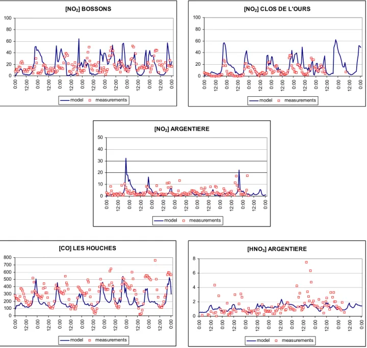
NO2 concentration at sites “Bossons”, “Clos de l’Ours”

and “Argenti`eres” leads to the same conclusion as for ozone (Fig. 8): only the south part of the valley is really affected

by traffic emissions. Concentrations of NO2decrease when

going to the north of the valley. Dilution of pollutants by wind transport is weak: important concentrations are

ob-served only close to the sources. NO2 correlations are

sat-isfactory but an improvement of the emission inventory for city and secondary traffic should improve results.

Nitric acid levels are low but well simulated (Fig. 8). CO concentration (Fig. 8) measured and simulated are more than 15 times inferior to the air quality norm (8591 ppb, on 8 h).

7 Photochemical indicators to distinguish ozone pro-duction regime

Narrow valleys in mountainous environment are very spe-cific areas when it comes to air quality. Emission sources

2350 G. Brulfert et al.: Modelling photochemistry in alpine valleys [O3] CHAMONIX CENTRE 0 20 40 60 80 100 0: 00 12 :0 0 0: 00 12 :0 0 0: 00 12 :0 0 0: 00 12 :0 0 0: 00 12 :0 0 0: 00 12 :0 0 0: 00 12 :0 0 0: 00 model measurements [O3] CLOS DE L'OURS 0 20 40 60 80 100 0: 00 12 :0 0 0: 00 12 :0 0 0: 00 12 :0 0 0: 00 12 :0 0 0: 00 12 :0 0 0: 00 12 :0 0 0: 00 12 :0 0 0: 00 model measurements [O3] BOSSONS 0 20 40 60 80 100 0: 00 12 :0 0 0: 00 12 :0 0 0: 00 12 :0 0 0: 00 12 :0 0 0: 00 12 :0 0 0: 00 12 :0 0 0: 00 12 :0 0 0: 00 model measurements [O3] BOIS DU BOUCHET 0 20 40 60 80 0: 00 12 :0 0 0: 00 12 :0 0 0: 00 12 :0 0 0: 00 12 :0 0 0: 00 12 :0 0 0: 00 12 :0 0 0: 00 12 :0 0 0: 00 model measurements [O3] ARGENTIERE 0 20 40 60 80 100 0: 00 12 :0 0 0: 00 12 :0 0 0: 00 12 :0 0 0: 00 12 :0 0 0: 00 12 :0 0 0: 00 12 :0 0 0: 00 12 :0 0 0: 00 model measurements [O3] PLAN DE L'AIGUILLE 0 20 40 60 80 100 0: 00 12 :0 0 0: 00 12 :0 0 0: 00 12 :0 0 0: 00 12 :0 0 0: 00 12 :0 0 0: 00 12 :0 0 0: 00 12 :0 0 0: 00 model measurements

[O3] COL DES MONTETS

0 20 40 60 80 100 0: 00 12 :0 0 0: 00 12 :0 0 0: 00 12 :0 0 0: 00 12 :0 0 0: 00 12 :0 0 0: 00 12 :0 0 0: 00 12 :0 0 0: 00 model measurements

Fig. 7. Concentrations of O3at different ground stations compared to results of the model (ppbV). Time on figures is universal time from 5

July to 11 July 2003 (IOP period).

[NO2] BOSSONS 0 20 40 60 80 100 0: 00 12 :0 0 0: 00 12 :0 0 0: 00 12 :0 0 0: 00 12 :0 0 0: 00 12 :0 0 0: 00 12 :0 0 0: 00 12 :0 0 0: 00 model measurements

[NO2] CLOS DE L'OURS

0 20 40 60 80 100 0: 00 12 :0 0 0: 00 12 :0 0 0: 00 12 :0 0 0: 00 12 :0 0 0: 00 12 :0 0 0: 00 12 :0 0 0: 00 12 :0 0 0: 00 model measurements [NO2] ARGENTIERE 0 10 20 30 40 50 0: 00 12 :0 0 0: 00 12 :0 0 0: 00 12 :0 0 0: 00 12 :0 0 0: 00 12 :0 0 0: 00 12 :0 0 0: 00 12 :0 0 0: 00 model measurements

[CO] LES HOUCHES

0 100 200 300 400 500 600 700 800 0: 00 12 :0 0 0: 00 12 :0 0 0: 00 12 :0 0 0: 00 12 :0 0 0: 00 12 :0 0 0: 00 12 :0 0 0: 00 12 :0 0 0: 00 model measurements [HNO3] ARGENTIERE 0 2 4 6 8 0: 00 12 :0 0 0: 00 12 :0 0 0: 00 12 :0 0 0: 00 12 :0 0 0: 00 12 :0 0 0: 00 12 :0 0 0: 00 12 :0 0 0: 00 model measurements

Fig. 8. Concentrations of CO, NO₂, HNO₃at different ground stations compared to results of the model (ppbV). Time on figures is universal time from 5 July to 11 July 2003 (IOP period).

are generally concentrated close to the valley floor, and very often include industries and transport infrastructures. For de-veloping ozone abatement strategies in a specific area, it is important to know whether the ozone production is limited

by VOC or NOx. In order to understand the impact of the

emissions sources on ozone production regime, three simu-lations are performed. All of them are based on meteorology and emission inventory of 6 July, 2003. Run B is the simu-lation of 7 July. Run N corresponds to an arbitrary reduction

in NOxemissions of 50%. Run V is obtained with an

arbi-trary reduction in VOC emissions of 50%. The three runs are described in Table 5.

This reduction of 50% of NOxcan be compared with the

traffic reduction between 1998 and 2001. The 50% decrease

in NOx roughly corresponds to the reduction observed

be-tween 1998 (with full transit traffic through the valley) and

2001 (no transit traffic): the main source of NOx in

sum-mer is traffic (Table 2). But a 10% VOC reduction only is associated to this traffic reduction.

7 July, 2003 is representative of a summer sunny day with mean pollution level. Photochemical indicators are

consid-ered in order to distinguishing NOxlimited and VOC limited

2352 G. Brulfert et al.: Modelling photochemistry in alpine valleys Bois du Bouchet y = 0.9895x - 1.7017 R2 _{= 0.7607} 0 10 20 30 40 50 60 70 80 0 20 40 60 80 ozone simulated (ppb) oz on e m es u re d (ppb)

Centre of Cham onix

y = 0.7869x + 8.5422 R2 _{= 0.7339} 0 10 20 30 40 50 60 70 80 0 20 40 60 80

ozone sim ulated (ppb)

oz on e me su re d (ppb) Clos de l'ours y = 0.9603x + 5.4484 R2 _{= 0.749} 0 10 20 30 40 50 60 70 80 0 20 40 60 80 ozone simulated (ppb) oz one m es u ra te d (ppb) Bois du Bouchet y = 0.9895x - 1.7017 R2 _{= 0.7607} 0 10 20 30 40 50 60 70 80 0 20 40 60 80 ozone simulated (ppb) oz on e m es u re d (ppb)

Centre of Cham onix

y = 0.7869x + 8.5422 R2 _{= 0.7339} 0 10 20 30 40 50 60 70 80 0 20 40 60 80

ozone sim ulated (ppb)

oz on e me su re d (ppb) Clos de l'ours y = 0.9603x + 5.4484 R2 _{= 0.749} 0 10 20 30 40 50 60 70 80 0 20 40 60 80 ozone simulated (ppb) oz one m es u ra te d (ppb) Bois du Bouchet y = 0.9895x - 1.7017 R2 _{= 0.7607} 0 10 20 30 40 50 60 70 80 0 20 40 60 80 ozone simulated (ppb) oz on e m es u re d (ppb)

Centre of Cham onix

y = 0.7869x + 8.5422 R2 _{= 0.7339} 0 10 20 30 40 50 60 70 80 0 20 40 60 80

ozone sim ulated (ppb)

oz on e me su re d (ppb) Clos de l'ours y = 0.9603x + 5.4484 R2 _{= 0.749} 0 10 20 30 40 50 60 70 80 0 20 40 60 80 ozone simulated (ppb) oz one m es u ra te d (ppb)

Fig. 9. Comparison between measured and simulated ozone in three

sites for the IPO.

Regional influence of O3.

Daily m ax compare w ith 'Col des Montets'

y = 0.8376x + 9.9723 R2 _{= 0.866} 50 55 60 65 70 75 80 50 60 70 80 Daily m ax of [O3] (ppb) [O 3] C o l d es Mo n tet s ( p p b )

Regional influence of O3.

Daily max compare w ith 'Plan de l'aiguille'

y = 0.8577x + 9.7326 R2 _{= 0.7907} 50 55 60 65 70 75 80 50 60 70 80

Daily max of [O3] (ppb)

[O 3] P la n d e l' ai g u ille ( ppb)

Regional influence of O3.

Daily m ax compare w ith 'Col des Montets'

y = 0.8376x + 9.9723 R2 _{= 0.866} 50 55 60 65 70 75 80 50 60 70 80 Daily m ax of [O3] (ppb) [O 3] C o l d es Mo n tet s ( p p b )

Regional influence of O3.

Daily max compare w ith 'Plan de l'aiguille'

y = 0.8577x + 9.7326 R2 _{= 0.7907} 50 55 60 65 70 75 80 50 60 70 80

Daily max of [O3] (ppb)

[O 3] P la n d e l' ai g u ille ( ppb)

Fig. 10. Comparison between daily maximum of O3(6 sites) and

concentration of O3at the same hour for background stations during

the IPO.

The indicators under consideration is NOy

(NOy=NOx+HNO3+PAN) (Milford et al., 1994). The

rationale for NOy as an indicator is based in part on the

impact of stagnant meteorology on NOx-VOC sensitivity.

Stagnant meteorology and associated high NOx, VOC, and

NOy cause an increase in the photochemical life times of

NOx and VOC, with the result that an aging urban plume

remains in the VOC-sensitive regime for a longer period of time. With more vigorous meteorological dispersion and

lower NOx, VOC and NOy an aging urban plume would

rapidly become NOxsensitive (Milford et al., 1994).

Figure 12 illustrates the NOx-VOC sensitivity for the

sim-ulations (runs N and V) in the bottom of the valley, every half an hour from 10:00 to 16:00 TU. Only meshes of the terrain with an altitude less than 1500 m above sea level are considered in order to include all the anthropogenic sources.

Fig. 11. Ozone concentration [ppb] and wind fields over Chamonix

valley at 12:00 (top) and 21:00 (bottom); 10 July 2003.

Although a significant part of the domain area is rural-type, effects of non rural emission predominate.

The Fig. 12 shows the change in ozone concentrations

as-sociated with either reduced VOC (run V) or reduced NOx

(run N) relative to the domain. The positive values represent locations where, by decreasing the emission, a reduction in ozone is obtained while negative values result from locations where reduced emissions cause more ozone.

According to the results, the ozone production is VOC lim-ited: only a diminution of VOC leads to a reduction of ozone concentration (run V).This conclusion differs from what was observed in the nearby city of Grenoble (100 km from the valley in a Y shape convergence of three deep valleys) where

a NOxcontrolled regime was observed (Couach et al., 2004).

Measurements of ozone between 1998 and 2001 in the town of Chamonix agree with this result with a 5 ppb increase of ozone concentration in summer. Nevertheless, this augmen-tation could be partly due to slight increase of regional con-centration.

Table 5. Runs to determine ozone production regime. The

reduc-tion of NOxor VOC emissions is applied to both anthropogenic and

biogenic sources.

Date Duration Emissions Run B 7 July 2003 24 h All

Run N 7 July 2003 24 h Run B – 50% NOx

Run V 7 July 2003 24 h Run B – 50% VOC

8 Conclusions

A system of models has been built to model dispersion and evolution of pollutants in narrow valleys. The methodology is applied to Chamonix valley but similar results were ob-tained, still in the frame of the POVA program, in Maurienne valley which lies 80 km from Chamonix but with signifi-cantly different topography (lower summits, wider extension, west-east oriented) (Brulfert, 2004). This system is based on several atmosphere dynamics and gas chemistry numerical codes selected for their ability to deal with processes devel-oping at different length and time scales. TAPOM and ARPS codes are used for fine space resolution when CHIMERE and MM5 are used at larger scales.

Three-dimensional photochemical simulations have been performed for a 7-day period with this system of models, during the POVA intensive period of observation in the topo-graphically complex and narrow Chamonix valley. Results from the numerical simulation are in good agreement with observations. Wind direction and forces are well reproduced with wind reversal observed at the same times in the model and from measurements. The evolution of the mixed layer thickness induced by thermal convection is well represented with growth in the morning and decay at night. These fea-tures of atmosphere dynamics are of major importance for transport and dilution of pollutants. Discrepancies on tem-perature and time of the wind shift are often due to the diffi-culties in parameterizing humidity and soil temperature. The model well simulates clear sky conditions which are predom-inant in summer polluted events.

Computed concentrations are in good agreement with measured values, for both primary and secondary pollutants. Correlation between maximum of ozone and background values (0.8) suggests the regional origin of the pollutant.

Di-lution of pollutants by wind transport (e.g. NO2) is weak:

im-portant concentrations are observed only close to the sources. In the upper valley, simulated and observed ozone concen-trations agree less than for the other stations, especially at night where the model underestimates the values because of

an overestimation of NOxin the emission inventory. Some

discrepancies in measurements and model results may be at-tributed to the “proximity” character of the station with high emissions and measurements in the same mesh of the model.

2354 G. Brulfert et al.: Modelling photochemistry in alpine valleys

NOy

-25

-20

-15

-10

-5

0

5

10

15

20

0

50

100

150

200

250

oz

o

n

e r

ed

u

ct

io

n (

p

pb

)

VOC controls

NOx controls

Fig. 12. NOyaccording to ozone reduction with NOxand VOC decrease (from 10:00 to 16:00 TU).

For a later purpose of suggesting reduction strategy, the general trend of chemical process has to be characterized. Well chosen indicators based on some species concentrations

allow to determine a prevailing mechanism. The NOy

indi-cator shows that the region of the maximum ozone is VOC saturated.

With the transfer of traffic from Chamonix to Maurienne valley because of the accident of Mont-Blanc tunnel, pro-gram POVA investigates also Maurienne. As for Chamonix valley, primary and secondary pollution is considered with measurements and numerical simulations based on the very same system of models. Ozone production regime and indi-cators obtained in the two valleys will be compared.

Acknowledgements. The program POVA is supported by “Air de l’Ain et des Pays de Savoie”, R´egion Rhˆone Alpes, ADEME, Primequal 2, METL, MEDD. Meteorological data are provided by M´et´eo France and ECMWF, traffic data by STFTR, ATMB, DDE Savoie et Haute Savoie. Computations were done on Mirage. TAPOM comes from the Air and Soil Pollution Laboratory of the Ecole Polytechnique F´ed´erale de Lausanne.

Edited by: L. M. Frohn

References

Ambrosetti, P., Anfossi, D., Cieslik, S., Graziani, G., Lamprecht, R., Marzorati, A., Nodop, K., Sandroni, S., Stingele, A., and Zimmermann, H.: Mesoscale transport of atmospheric trace

con-stituents across the central alps: TRANSALP tracer experiments, Atmos. Environ., 32(7), 1257–1272, 1998.

Anquetin, S., Guilbaud, C., and Chollet, J. P.: Thermal valley inver-sion impact on the disperinver-sion of a passive polluant in a complex mountainous area, Atmos. Environ., 33, 3953–3959, 1999. Brulfert, G., Chollet, J. P., Jouve, B., and Villard, H.: Atmospheric

emission inventory of the Maurienne valley for an atmospheric numerical model, Sci. Total Environ., in press, 2005.

Brulfert, G.: Mod´elisation des circulations atmosph´eriques pour l’´etude de la pollution des vall´ees alpines, Thesis manuscript, 263 pp., available on http://tel.ccsd.cnrs.fr/documents/archives0/ 00/00/79/82/index fr.html, University Joseph Fourier, Grenoble, France, 2004.

Chaxel, E., Brulfert, G., Chemel, C., and Chollet, J. P.: Evalua-tion of local ozone producEvalua-tion of Chamonix valley (France) dur-ing a regional smog episode. 27th NATO/CCMS International Technical Meeting on Air Pollution Modelling and its Applica-tion Banff, Canada, available on: http://www.dao.ua.pt/itm/27th/ Presentations, 25–29 October 2004.

Clappier, A.: A correction method for use in multidimensional time splitting advection algorithms: application to two and three di-mensional transport, Mon. Wea. Rev., 126, 232–242, 1998. Couach, O., Balin, I., Jim´enez, R., Ristori, R., Kirchner, F., Perego,

S., Simeonov, V., Calpini, B., and Van den Bergh, H: Investiga-tion of the ozone and planetary boundary layer dynamics on the topographically-complex area of Grenoble by measurements and modeling, Atmos. Chem. Phys., 3, 549–562, 2003,

SRef-ID: 1680-7324/acp/2003-3-549.

Couach, O., Kirchner, F., Jimenez, R., Balin, I., Perego, S., and Van den Bergh, H.: A development of ozone abatement strategies

Environ., 38, 1425–1436, 2004.

Espace Mont Blanc: Technical report of the study Air Espace Mont Blanc, 147 pp., available at http://www.espace-mont-blanc.com, 2003.

Gong, W. and Cho, H.-R.: A numerical scheme for the integration of the gas phase chemical rate equations in a thre-dimensional at-mospheric models, Atmos. Environ., 27A(14), 2147–2160, 1993. Grell, G. A., Dudhia, J., and Stauffer, D. R.: A description of the Fifth-Generation Penn State/ NCAR Mesosale Model (MM5). NCAR technical note NCAR/TN-398+STR, NCAR, Boulder, CO. 117 pp., 1995.

Grell, G. A., Emeis, S., Stockwell, W. R., Schoenemeyer, T., Forkel, R., Michalakes, J., Knoche, R., and Seidl, W.: Application of a multiscale coupled MM5/chemistry model to the complex terrain of the VOTALP valley campaign, Atmos. Environ., 34(9), 1435– 1453, 2000.

Jimenez, P., Baldasano, J. M, Dabdub, D.: Comparaison of photo-chemical mechanisms for air quality modeling, Atmos. Environ., 37, 4179–4194, 2003.

Lehning, M., Richner, H., and Kok, G. L.: Pollutant transport over complex terrain: flux and budget calculations fort he POL-LUMET field campaign, Atmos. Environ., 30(17), 3027–3044, 1996.

L¨offler-Mang, M., Zimmermann, H., and Fiedler, F.: Analysis of ground based operational network data acquired during the September 1992 TRACT campaign, Atmos. Environ., 32(7), 1229–1240, 1998.

and analysis of volatile organic compound emissions for regional modeling, Atmos. Environ., 241(5), 1107–1133, 1990.

Milford, J. B. and Gao, D.: Total reactive nitrogen (NOy) as an

indicator of the sensitivity of ozone to reductions in hydrocarbon and NOxemissions, J. Geophys. Res., 99(D2), 3533–3542, 1994.

Schmidt, H., Derognat, C., Vautard, R., and Beekmann, M.: A com-parison of simulated and observed ozone mixing ratios for the summer of 1998 in Western Europe, Atmos. Environ., 35, 6277– 6297, 2001.

Stockwell, R., Kirchner, F., Kuhn, M., and Seefeld, S.: A new mechanism for atmospheric chemistry modelling, J. Geophys. Res., 102(D22), 25 847–25 879, 1997.

Wotawa, G. and Kromp-Kolb, H.: The research project VOTALP – general objectives and main results, Atmos. Environ., 34(9), 1319–1322, 2000.

Xue, M., Droegemeir, V., and Wong, V.: The Advanced Regional Prediction System (ARPS)– A multi-scale nonhydrostatic atmo-spheric simulation and prediction model. Part I: Model dynamics and verification, Met. Atm. Phys., 75(3), 161–193, 2000. Xue, M., Droegemeir, K. K., Wong, V., Shapiro, A., Brewster, K.,

Carr, F., Weber, D., Liu, Y., and Wang, D.: The advanced re-gional prediction system (arps) – a multi-scale non hydrostatic at-mospheric simulation and prediction tool. Part ii: Model physics and applications, Met. Atm. Phys., 76, 143–165, 2001.