Down-the-barrel observations of a multi-phase quasar outflow at high redshift

HAL Id: hal-03143632

https://hal.archives-ouvertes.fr/hal-03143632

Submitted on 16 Feb 2021

HAL is a multi-disciplinary open access

archive for the deposit and dissemination of

sci-entific research documents, whether they are

pub-lished or not. The documents may come from

teaching and research institutions in France or

abroad, or from public or private research centers.

L’archive ouverte pluridisciplinaire HAL, est

destinée au dépôt et à la diffusion de documents

scientifiques de niveau recherche, publiés ou non,

émanant des établissements d’enseignement et de

recherche français ou étrangers, des laboratoires

publics ou privés.

Down-the-barrel observations of a multi-phase quasar

outflow at high redshift

P. Noterdaeme, S. Balashev, J.-K. Krogager, P. Laursen, R. Srianand, N.

Gupta, P. Petitjean, J. P. U. Fynbo

To cite this version:

P. Noterdaeme, S. Balashev, J.-K. Krogager, P. Laursen, R. Srianand, et al.. Down-the-barrel

observa-tions of a multi-phase quasar outflow at high redshift: VLT/X-shooter spectroscopy of the proximate

molecular absorber at z = 2.631 towards SDSS J001514+184212. Astronomy and Astrophysics - A&A,

EDP Sciences, 2021, 646, pp.A108. �10.1051/0004-6361/202038877�. �hal-03143632�

https://doi.org/10.1051/0004-6361/202038877 c P. Noterdaeme et al. 2021

Astronomy

&

Astrophysics

Down-the-barrel observations of a multi-phase quasar outflow at

high redshift

VLT/X-shooter spectroscopy of the proximate molecular absorber at z = 2.631

towards SDSS J001514+184212

?

P. Noterdaeme

1

, S. Balashev

2

, J.-K. Krogager

1

, P. Laursen

3,4

, R. Srianand

5

, N. Gupta

5

,

P. Petitjean

1

, and J. P. U. Fynbo

4,6

1 _{Institut d’Astrophysique de Paris, CNRS-SU, UMR 7095, 98bis bd Arago, 75014 Paris, France}

e-mail: noterdaeme@iap.fr

2 _{Ioffe Institute, Polyteknicheskaya 26, 194021 Saint-Petersburg, Russia}

3 _{Institute of Theoretical Astrophysics, University of Oslo, PO Box 1029, Blindern 0315, Oslo, Norway} 4 _{Cosmic Dawn Center (DAWN), University of Copenhagen, Jagtvej 128, 2200 Copenhagen N, Denmark}

5 _{Inter-University Centre for Astronomy and Astrophysics, Pune University Campus, Ganeshkhind, Pune 411007, India} 6 _{Niels Bohr Institute, University of Copenhagen, Jagtvej 128, 2200 Copenhagen N, Denmark}

Received 8 July 2020/ Accepted 3 December 2020

ABSTRACT

We present ultraviolet to near infrared spectroscopic observations of the quasar SDSS J001514+184212 and its proximate molecu-lar absorber at z = 2.631. The [O

_iii

] emission line of the quasar is composed of a broad (FWHM ∼ 1600 km s−1_{), spatially}

unre-solved component, blueshifted by about 600 km s−1_{from a narrow, spatially-resolved component (FWHM ∼ 650 km s}−1_{). The wide,}

blueshifted, unresolved component is consistent with the presence of outflowing gas in the nuclear region. The narrow component can be further decomposed into a blue and a red blob with a velocity width of several hundred km s−1_{each, seen ∼5 pkpc on opposite}

spatial locations from the nuclear continuum emission, indicating outflows on galactic scales. The presence of ionised gas on kpc scales is also seen from a weak C

_iv

emission component, detected in the trough of a saturated C

_iv

absorption that removes the strong nuclear emission from the quasar. Towards the nuclear emission, we observe absorption lines from atomic species in various ionisation and excitation stages and confirm the presence of strong H2lines originally detected in the SDSS spectrum. The overall

absorption profile is very wide, spread over ∼600 km s−1_{, and it roughly matches the velocities of the narrow blue [O}

iii

] blob. From a detailed investigation of the chemical and physical conditions in the absorbing gas, we infer densities of about nH∼ 104−105cm−3in

the cold (T ∼ 100 K) H2-bearing gas, which we find to be located at ∼10 kpc distances from the central UV source. We conjecture that

we are witnessing different manifestations of a same AGN-driven multi-phase outflow, where approaching gas is intercepted by the line of sight to the nucleus. We corroborate this picture by modelling the scattering of Ly-α photons from the central source through the outflowing gas, reproducing the peculiar Ly-α absorption-emission profile, with a damped Ly-α absorption in which red-peaked, spatially offset, and extended Ly-α emission is seen. Our observations open up a new way to investigate quasar outflows at high redshift and shed light on the complex issue of AGN feedback.

Key words. quasars: emission lines – quasars: absorption lines – quasars: individual: SDSS J001514.82+184212.34

1. Introduction

Feedback from active galactic nuclei (AGN) is an essential element in modern models of galaxy formation and evolu-tion (e.g., Silk & Rees 1998). It may quench star formation (e.g.,Zubovas & King 2012;Pontzen et al. 2017;Terrazas et al. 2020), impact galaxy morphology (Dubois et al. 2016), regu-late the growth of the supermassive black holes (Volonteri et al. 2016), and so on. It may also have positive feedback on star formation through compression of the gas (e.g.,Zubovas et al. 2013; Richings & Faucher-Giguère 2018). The most support-ive evidence for AGN feedback is the presence of kiloparsec-scale outflows, which result from the propagation of energy and momentum from accretion disc winds to the host galaxy ? _{Based on observations collected at the European Organisation for}

Astronomical Research in the Southern Hemisphere under ESO pro-gramme 103.B-0260(A).

interstellar medium (e.g., Fabian 2012; Costa et al. 2015). At low and intermediate redshifts, such outflows have been observed in ionised and molecular phases, with many stud-ies focusing on Type 2 quasars, where the obscuration of the nuclear emission facilitates the observations (e.g., Sun et al. 2017). Outflows have also been observed in unobscured, lumi-nous AGN (Type 1 quasars), but mostly at low redshift, such as the well-known Mrk 231 at z = 0.04 (Rupke & Veilleux 2011; Feruglio et al. 2015). Naturally, observational constraints on hot and cold outflows in high-redshift Type 1 quasars are much harder to obtain, not only because of the dimming of the light, but also because the coarser angular resolution impedes obser-vations close to the bright nucleus.

In turn, the cosmological distances and high luminosity of the nuclear emission of high-z quasars make them excellent background sources against which gas in any phase can be stud-ied in absorption. This includes not only gas at any place along

Open Access article,published by EDP Sciences, under the terms of the Creative Commons Attribution License (https://creativecommons.org/licenses/by/4.0),

Table 1. Log of observations and atmospheric parameters.

Date Slit position angle (PA) Seeing Airmass R(H2O)(a) R(CO2)(a) FWHM(NIR)(b)

(deg E. of N.) (arcsec) (pixel)

2019-07-29 +166 1.67 1.48 1.10 1.44 4.3

2019-08-31 −164 0.75 1.39 0.86 1.25 3.0

2019-08-31 +177 0.65 1.41 0.91 1.30 2.9

2019-09-28 −155 0.53 1.42 0.94 1.04 3.8

Notes.(a)_{Best-fitting relative abundance compared to the default template in molecfit: N(H}

2O)= 2.725 × 104ppmv and N(CO2)= 368.5 ppmv.

Typical uncertainties of ∼0.01.(b)_{Best-fit spectral resolution of the NIR spectrum from molecfit with typical uncertainties of 0.1 pixel.}

the line of sight (from the intergalactic medium, giving rise to the Ly-α forest or closer to intervening galaxies, producing damped Ly-α systems (DLAs) in the quasar spectrum), but also gas close to the supermassive black hole, in the quasar host galaxy or in galaxies belonging to the quasar group environment. While broad absorption lines have long been associated with gas flows close to the central engine (e.g.,Weymann et al. 1991; Arav et al. 2018), large-scale outflows, when intercepted by the line of sight to the nucleus, should also produce a detectable sig-nature in absorption.

Absorption spectroscopy has proven to provide very detailed information about the kinematics, chemical composition, and physical conditions in the absorbing gas, in particular when molecules are detected. Indeed, the formation, survival, and excitation of molecules is very sensitive to the prevailing physi-cal conditions, such as abundance of dust, temperature, density, and ambient UV field (e.g.,Reimers et al. 2003;Srianand et al. 2005;Cui et al. 2005;Guillard et al. 2009;Balashev et al. 2017; Wakelam et al. 2017, among many others).

Combining information from both emission and absorption line measurements could hence provide us with a fresh view of quasar outflows and feedback at high redshift. We recently embarked on a search for damped molecular hydrogen (H2)

absorption lines at the quasar redshift in low-resolution spec-tra from the Sloan Digital Sky Survey (SDSS) III (BOSS) Data Release 14. Through this targeted search, we discovered a popu-lation of strong proximate H2absorption systems at z > 2.5 with

log N(H2) > 19 (Noterdaeme et al. 2019). Detailed follow-up

observations are currently on-going using the multi-wavelength spectrograph X-shooter on the Very Large Telescope (VLT).

In this paper, we report on the observations of the first object in our sample, the quasar SDSS J001514.82+184212.34 (here-after J0015+1842) at z = 2.63. We interpret the observations as evidence of kilo-parsec scale, multi-phase, biconical out-flows that are mainly orientated along the line of sight and also probed in absorption against the nucleus. We present the obser-vations and data reduction in Sect.2, the analysis of spatially-resolved emission lines in Sect. 3, and that of absorption lines and dust extinction towards the nucleus in Sect. 4. We discuss our results in Sect.5, along with the derivation of the chemical and physical conditions in the absorbing clouds and the mod-elling of leaking Ly-α emission. We summarise our findings in Sect.6. Throughout this paper, we assume a flatΛCDM cosmol-ogy with H0 = 68 km s−1Mpc−1,ΩΛ = 0.69, and Ωm = 0.31

(Planck Collaboration XIII 2016).

2. Observations and data reduction

J0015+1842 was observed in stare mode with the X-shooter spectrograph at the VLT at the Paranal Observatory in Chile

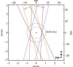
−3 −2 −1 0 1 2 3 arcsec −3 −2 −1 0 1 2 3 arcsec −155 o N E +177o N E −164o N E +166o N E −20 −10 kpc0 10 20 −20 −10 0 10 20 kpc BOSS fiber Fig. 1.Layout of 1.200

-wide X-shooter slits in the NIR. The small dotted circle represents a projected area of radius 5 kpc (at the redshift of the quasar) with 100% coverage by all our X-shooter slit positions, and the larger dashed circle represents the BOSS fibre aperture.

between July and September 2019. The log of observations is provided in Table1.

The X-shooter spectrograph simultaneously covers the wavelength range from 0.3 to 2.5 µm in three separate spectro-graphs, which are the so-called arms: UVB ranging from 0.3 to 0.6 µm; VIS ranging from 0.6 to 1.0 µm; and NIR ranging from 1.0 to 2.5 µm. For all observations, slit widths of 1.0, 0.9, and 1.2 arcsec were used for the UVB, VIS, and NIR arms, respec-tively. The slit was aligned to the parallactic angle at the start to minimise slit losses of the exposure, and it was kept fixed on sky during the ∼1 h long exposure (see Fig. 1). The obser-vation from August 30 failed due to an error in the atmospheric dispersion corrector (ADC), and exposures from this date were therefore not included in the analysis. For one other observation (July 29), we noted a strong chromatic suppression of flux in the UVB arm1_{, hence the UVB spectrum from this observation}

has been discarded from our analysis. As the loss of flux in the VIS and NIR arms is much less severe, we used these spectra in our analysis but weighted them appropriately (using the inverse variance) when combining the individual spectra.

The raw spectra were processed using the official esorex pipeline for X-shooter version 2.6.8. Before passing the raw spectra through the pipeline, we corrected cosmic ray hits using 1 _{The chromatic slit loss is most likely due to the poor seeing (1.7}00

); however, it may also be related to a partial failure of the ADC for the UVB arm.

the code A

_stroscrappy

(McCully et al. 2018), which is a Python implementation of the algorithm byvan Dokkum(2001). The pipeline then performed subtraction of bias and dark levels on the CCD, spectral flat fielding, tracing of the curved echelle orders, and computation of the wavelength solution. The indi-vidual curved 2D orders were then rectified onto a straightened grid. The sky background was subsequently subtracted before the individual orders were combined. The full spectrum was flux-calibrated using a sensitivity function calculated for each observation using a spectroscopic standard star observed during the same night. The three spectra (UVB, VIS, NIR) were stitched together in the overlapping regions, correcting for any small o ff-sets between the absolute flux calibration of the individual arms. Lastly, in order to correct for possible slit loss, we scaled the cal-ibrated spectra to match the SDSS i band photometry. Because of the possible variation of the quasar brightness between the time of observation for the SDSS photometry and our data, the abso-lute flux calibration has a systematic uncertainty of order 20%, which corresponds to the typical long-term variability of quasars (Hook et al. 1994).

From the 2D spectra produced by the pipeline, we per-formed an optimal extraction (Horne 1986) to obtain 1D spec-tra. The 1D and 2D spectra were subsequently corrected to vacuum wavelengths and shifted to the heliocentric reference frame before being corrected for Galactic extinction using the maps bySchlafly & Finkbeiner(2011). Lastly, we combined the individual observations for each arm into final 1D spectra using a weighted mean.

Telluric correction. The NIR spectra were corrected for tel-luric absorption using the software tool molecfit (Smette et al. 2015;Kausch et al. 2015). The code fits a synthetic absorption profile to the telluric absorption features in the data. For the NIR spectra, the dominant molecular species giving strong telluric absorption lines are H2O and CO2. The relative abundances of

these two species were fitted together with a fifth-order poly-nomial model for the intrinsic spectrum in order to reproduce the shape of the wings of the quasar emission lines. We fitted the telluric model using seven narrow bands of the spectra dom-inated by telluric absorption features only. These seven regions were chosen to encompass regions of interest, that is, the regions around the quasar emission lines from oxygen. The wavelength intervals used were as follows: 1.13–1.14, 1.37–1.39, 1.44–1.45, 1.75–1.76, 1.82–1.83, 1.94–1.97, and 2.02–2.03 µm. For each region, we iteratively masked out pixels affected by skyline residuals or bad pixels. The optimal parameters for each spec-trum are given in Table 1. The optimised telluric absorption model for each spectrum was then used to correct the corre-sponding 1D and 2D spectra.

3. Emission line analysis

We analysed the 1D and 2D together spectra to extract infor-mation about the spatial and spectral properties of the vari-ous emission lines of interest. In addition to the 1D spectrum obtained through the optimal extraction method, which mostly samples the unresolved nuclear emission (due to the weighting profile), we also constructed a total 1D NIR spectrum directly extracted from the combined 2D data over a wider spatial range of ±9 pixels (or equivalently 1.9 arcsec) around the quasar trace without weighting. This is specifically constructed for the anal-ysis of spatially extended emission lines such as [O

_iii

]. In sum-mary, we therefore consider three kinds of 1D spectra in the fol-lowing: (i) the on-trace spectrum, which is obtained from the

1.33 1.34 1.35 1.36 1.37 1.38 Observed wavelength (µm) 0 1 2 3 Fλ (10 −17 erg s −1 cm −2 Å −1) [OII]

Fig. 2.Portion of combined 1D NIR spectrum around the [O

_ii

] dou-blet emission line. The 1D spectrum with (without) telluric correction is shown in black (orange) together with the fitted profile in red.

trace by optimal extraction; (ii) the overall spectrum, which is extracted within wide spatial range; and (iii) the off-trace spec-trum, which is the difference between the two others.

3.1. [O ii]

The [O

_ii

]λλ3727, 3729 doublet is redshifted into a strong tel-luric band and not directly visible in the original data. However, applying the telluric correction described in Sect.2 allowed us to recover the lines, which, given their large velocity width, are strongly blended and appear as a single line in Fig.2. To esti-mate the intrinsic line width we fitted the [O

_ii

] doublet using the sum of two Gaussians plus a linear continuum in that region. The relative positions of the Gaussians were kept fixed to the doublet wavelength ratio, and their widths were forced to be the same. In principle, the amplitude ratio for the [O

_ii

] doublet can vary between 0.35 and 1.5, depending on the kinetic temperature of the gas and the electron density (e.g.,Kisielius et al. 2009). However, because this region of the spectrum is quite noisy, we assumed a fixed ratio of 1.3. This assumption has almost no influence on the total line flux and width. The obtained parame-ters are given in Table2. We measured the [O

_ii

] emission red-shift to be z= 2.631.

3.2. [O iii] and H β

We analysed the H β and [O

_iii

]λλ4960,5008 lines simultane-ously, since these lines are located in the same region from 1.74 to 1.84 µm. Both the Hβ and the [O

_iii

] profiles are found to be non-Gaussian and spread over about 2000 km s−1. The forbid-den [O

_iii

]λλ4960, 5008 emission lines are clearly asymmetric, and composed of a broad and ‘narrow’ component separated by about 600 km s−1_{. We found that the overall Hβ+[O}

iii

] complex can be well modelled by the sum of a smooth continuum com-ponent (green line in Fig.3) and six Gaussian profiles, two for each spectral line (purple and brown for Hβ; orange and blue for the [O

_iii

] doublet). Because [O

_iii

] lines can only be deex-cited radiatively and since their upper energy levels are only slightly different, the [O

_iii

] line ratio remains constant. There-fore, to fit these lines we tied the redshifts and line widths for the two [O

_iii

] lines and imposed their amplitude to follow the theo-retical 1:3 ratio (e.g.,Storey & Zeippen 2000;Dimitrijevi´c et al. 2007). Since the narrow [O

_iii

] component is spatially resolved (see Sect.3.4), we considered the overall 1D spectrum instead of the on-trace spectrum when fitting this line. We also used the off-trace spectrum to obtain an initial guess for the parameters of the narrow component free from contamination by the broad

Table 2. Emission line parameters. Line z FWHM L (km s−1) (1044erg s−1) Hβ, comp 1 2.6252 5700 ± 430 0.9 Hβ, comp 2 2.6273 1960 ± 150 0.5 [O

_iii

]λ5008, broad 2.6233 1600 ± 60 1.1 [O

_iii

]λ5008, narrow 2.6309 630 ± 50 0.6 [O

_ii

] 2.6310 950 ± 80 0.15 C

_iv

, comp 1 2.6149 5620 ± 170 1.3 C

_iv

, comp 2 2.6221 2050 ± 50 0.6 Leaking Lyα 2.634 600 1.4

Notes. The apparent peak and FWHM of the leaking Ly-α emission were estimated visually from the non-Gaussian spectral profile and the luminosity from direct integration. For the other lines, these parameters were obtained from fitting the Gaussian profiles as described in the text. Statistical uncertainties on the line luminosities are about 10% for NIR lines and 5% for UVB lines. However, the uncertainty on the absolute flux calibration is about 20%. This has no effect on the line ratios.

1.74 1.76 1.78 1.80 1.82 1.84 Observed wavelength (µm) 0 2 4 6 8 Fλ (10 −17 erg s −1 cm −2 Å −1) overall overall Hβ Hβ [OIII] [OIII] 0 1 2 3 4 off−trace only off−trace only

Fig. 3.Portion of combined 1D NIR spectrum around Hβ and [O

_iii

] emission lines. Top panel: contribution from the off-trace spatially extended emission, which is apparent in both [O

_iii

] lines. Bottom panel: spectrum collapsed over its full spatial extent at wavelengths 1.790 < λ(µm) < 1.825 and the optimal extraction elsewhere, for pre-sentation purposes. The green line shows our estimate of featureless continuum emission. Individual Gaussians constrained during the fit are shown in different colours, with the total fitted profile shown in red.

nuclear component (top panel of Fig.3). We then fitted the over-all spectral profile relaxing over-all parameters and rejecting deviating pixels iteratively. The corresponding line parameters are given in Table2.

The peak of the narrow [O

_iii

] emission provides us with an estimate of the quasar host’s systemic redshift, which also matches that obtained from [O

_ii

]. Given the associated uncer-tainty of about 100 km s−1, we rounded the value to z= 2.631, which we take as a convenient reference redshift to define the zero point of our velocity scale throughout this work.

3.3. C iv emission

The region of 1D spectrum around the C

_iv

emission line is shown in Fig. 4. Strong absorption from the proximate DLA

Observed wavelength (Å) 5600 5610 5620 5630 5640 5650 −3 −2 −10 1 2 3 arcsec 5500 5550 5600 5650 5700 5750 Observed wavelength (Å) 0 2 4 6 8 Fλ (10 −17 erg s −1 cm −2 Å −1) CIV 5615 5620 5625 5630 −0.10.0 0.1 0.2 0.3

Fig. 4.Bottom: portion of 1D X-shooter spectrum around the C

_iv

emis-sion line, median-smoothed using a 5-pixel sliding window for presen-tation purposes (black, with 1σ error level in green). The inset shows an unsmoothed zoom-in on the C

_iv

absorption, with the blue region high-lighting the residual emission. The best-fit model is shown by the red solid line and the individual Gaussians as red dotted lines. The down-wards arrow indicates the systemic redshift. Top: 2D spectrum in the region featuring the C

_iv

absorption line as well as residual C

_iv

emis-sion in the trough.

(PDLA) is observed in the red wing of the emission line. We fitted the emission line using the sum of two Gaussians plus a linear continuum in that region, excluding the region affected by absorption. The C

_iv

emission peaks at ∼5611 Å, while the C

_iv

absorption is centred at ∼5625 Å. Furthermore, the C

_iv

emis-sion is shifted by about 700 km s−1 _{bluewards of the systemic}

redshift but matches the location of the broad [O

_iii

] compo-nent well. Interestingly, while the shape and strength of the C

_iv

absorption profile indicate strong saturation, a residual emis-sion is seen in the trough, with a possible peak at the systemic velocity. Even though the value for each pixel remains rela-tively close to the noise level, the residual emission is consis-tently seen above zero for almost all pixels, with integrated flux Fresi∼ (1.3 ± 0.1) × 10−17erg s−1cm−2, that is, 13σ significance.

In principle, we cannot rule out that this is due to the absorption profile being composed of a blend of many narrow unsaturated components. We note, however, that reproducing the sharp edges and the width of the profile while keeping the non-zero absorp-tion in the centre is very difficult, even more so with the condi-tion that the C

_iv

column density be bounded by the metallicity. A more likely explanation is that the C

_iv

emission is not fully covered by the C

_iv

absorbing gas. This is corroborated by the spatial extent of the residual emission, which is discussed in the following sub-section.

3.4. Spatial extent of line-emitting regions

The spatial profiles of the [O

_ii

], [O

_iii

], Hβ and C

_iv

emission lines are compared to that of the continuum in Fig.5. These were obtained by collapsing the combined 2D spectrum along the wavelength axis around each line, while rejecting outlying pixels (due to telluric residuals or bad pixels). The regions for collaps-ing the data were chosen as follows. For [O

_ii

] and Hβ, we col-lapsed the data in a region centred at the peak of each line using a width matching the measured FWHM. Since the [O

_iii

] profile

is very asymmetric, we considered two regions representative of the broad and narrow components separately. To investigate the spatial profile around the narrow [O

_iii

] component, we again used a region centred at the peak position within one FWHM. However, to assess whether the photons from the broad com-ponent come from compact (unresolved) or spatially extended regions, we restricted the region to 1.805−1.815 µm. This avoids contamination by the narrow component. In the case of C

_iv

, we collapsed the data over the 5580−5650 Å region, which roughly corresponds to the FWHM centred at the line peak. We also col-lapsed the data in the 5619−5628 Å region, corresponding to the region of the C

_iv

absorption trough where some residual emis-sion is seen (Fig.4).

We found that the spatial profiles of [O

_ii

], H β the broad [O

_iii

], and the overall C

_iv

emission are unresolved, perfectly matching the spatial profile of the continuum and hence mostly originating from the nuclear region. In turn, the narrow [O

_iii

] line is significantly extended, over several kpc, on both sides of the trace of the continuum. The C

_iv

absorption trough acts like a natural coronagraph, removing the bright quasar glow at these wavelengths. This provides easier access to extended but fainter C

_iv

emission. While it is hard to appreciate the spatial profile of the residual (weak) C

_iv

emission from the 2D data (top panel of Fig.4), when collapsing along the wavelength axis, and albeit still noisy, this profile clearly presents a spatial kpc-scale exten-sion below the trace.

In order to further characterise the extension of the narrow [O

_iii

] emission line, we show the individual 2D spectra in Fig.6, with and without subtraction of the smooth continuum and broad emission. The extended narrow [O

_iii

] emission appears as blobs both above and below the quasar trace, with very similar loca-tions and extents for all position angles (PA). This is not very surprising given the small differences in PAs (due to the observa-tions always being taken with the slit aligned to parallactic angle; see Fig. 1). However, we noticed that the observed fluxes are higher for PA= +177 deg and PA = −164 deg than for the other position angles. This suggests that slit losses could be at play for PA= 155 deg and +166 deg, and hence the extended emission is oriented close to the north-south direction.

In Fig. 7, we show the average spatial profile in three velocity bins around our reference redshift (v (km s−1) = [−300, −100]; [−100,+100]; [+100, +300]) after removing the unresolved continuum+broad [O

_iii

] emission. The centroids of the both blue and red blobs are at projected distances ∼4−6 pkpc from the nuclear emission. In addition, the centre and the blue wing of the narrow [O

_iii

] emission extend from the nucleus up to large distances. While part of these spatial extents are due to the smearing effect of the seeing, it clearly indicates that [O

_iii

] emission extends over at least ∼10 pkpc from the central engine. We remark that the [O

_iii

] emission extends above and below the trace for roughly negative and positive velocities (according to our reference redshift), respectively.

3.5. The Ly-α emission

The spectrum of J0015+1842 in the Ly-α region is the sum of the quasar emission absorbed by the proximate DLA and the leak-ing Ly-α emission superimposed on the DLA trough, as already mentioned in our discovery work (Noterdaeme et al. 2019). One difficulty with the low-resolution, low signal-to-noise ratio (S/N) BOSS fibre spectrum was to ascertain the combined model of absorption and emission since the quasar redshift was not easily determined and the wings of the DLA were not clearly detected. The higher quality X-shooter spectrum confirms our previous

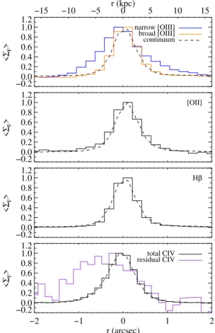
−0.20.0 0.2 0.4 0.6 0.8 1.0 1.2 < ΣF > narrow [OIII] broad [OIII] continuum −15 −10 −5 r (kpc)0 5 10 15 −0.20.0 0.2 0.4 0.6 0.8 1.0 1.2 < ΣF > [OII] −0.20.0 0.2 0.4 0.6 0.8 1.0 1.2 < ΣF > Hβ −2 −1 0 1 2 r (arcsec) −0.20.0 0.2 0.4 0.6 0.8 1.0 1.2 < ΣF > total CIV residual CIV

Fig. 5.Average observed spatial profiles at the location of different

emission lines. In each panel, the dashed curve shows the spatial point spread function obtained from the quasar continuum in a nearby region. We note that the profile around the narrow [O

_iii

] emission still contains a contribution from the continuum and the broad [O

_iii

] emission. For the sake of easy comparison, each profile is normalised by its maximum value.

decomposition (see Fig.8). The absorption profile is well con-strained by the damping wings of the DLA as well as other lines from the Lyman series, which were fitted simultaneously with H2

lines (Fig.10). The intrinsic quasar emission profile was recon-structed simultaneously using a smooth spline profile, aided by the quasar template matching (see Sect.4.5); however, the exact shape of the peak is highly uncertain since it is positioned at the same place as the DLA trough. Nonetheless, we note that the exact shape and strength of the intrinsic, broad Ly-α emission line has little influence on the analysis presented in this paper.

In Fig. 8, we also show the original BOSS spectrum. The residual Ly-α emission appears nearly two times stronger in the BOSS spectrum than in the X-shooter spectrum. The reason is that the optimal extraction method used for the X-shooter spec-trum gives lower weight to the extended and spatially offset Ly-α emission. Instead, the 2D spectra clearly show that the residual Ly-α emission is spatially offset and extended (Fig.9), and the overall (non-optimal) X-shooter extraction does match the SDSS data (top-right panel of that figure) much better. This will be dis-cussed in the following.

Since the system was identified through its H2 absorption

lines imprinted on the quasar continuum, the absorbing gas inter-cepts the line of sight to the central engine, removing the unre-solved emission and leaving us with a perfect PSF subtraction of the nuclear emission over the saturated region (∼4405−4420 Å

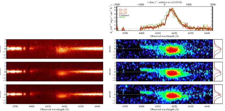
0 2 4 6 8 Fλ (10 −17 erg s −1 cm −2 Å −1) −2000 −1500 −1000 −500 0 500 1000 1500 2000 v (km s−1_{, relative to z=2.6310)} 1.810 1.815 1.820 1.825 1.830 −2 −1 0 1 2 arcsec −2000 −1500 −1000 −500 0 500 1000 1500 2000 1.810 1.815 1.820 1.825 1.830 −2 −1 0 1 2 arcsec −2000 −1500 −1000 −500 0 500 1000 1500 2000 1.810 1.815 1.820 1.825 1.830 −2 −1 0 1 2 arcsec −2000 −1500 −1000 −500 0 500 1000 1500 2000 1.810 1.815 1.820 1.825 1.830 −2 −1 0 1 2 arcsec −2000 −1500 −1000 −500 0 500 1000 1500 2000 1.810 1.815 1.820 1.825 1.830 −2 −1 0 1 2 arcsec −2000 −1500 −1000 −500 0 500 1000 1500 2000 1.810 1.815 1.820 1.825 1.830 −2 −1 0 1 2 arcsec −2000 −1500 −1000 −500 0 500 1000 1500 2000 Observed wavelength (µm) 1.810 1.815 1.820 1.825 1.830 −2 −1 0 1 2 3 arcsec −2000 −1500 −1000 −500 0 500 1000 1500 2000 Observed wavelength (µm) 1.810 1.815 1.820 1.825 1.830 −2 −1 0 1 2 3 arcsec −2000 −1500 −1000 −500 0 500 1000 1500 2000

Fig. 6.Individual 2D spectra around the [O

iii

]λ5008 region (from top to bottom: PA= −155 deg, −164 deg, +177 deg, and +166 deg east of north, i.e. in these figures, north is down and south is up). The total observed emission is shown in the left panels, while the unresolved emission (continuum+broad component) has been subtracted in the right panels to better highlight the spatially-extended narrow [O

iii

] emission alone. Each panel is 4000 km s−1_{wide. The main skyline residuals are masked out by a white hashed grid. Top-left panel: total extracted 1D spectrum,}

with the corresponding Gaussian fits. The coloured regions show the velocity bins used in Fig.7.

−20 −10 0 10 20 r (kpc) 0 5 10 15 20 25 ΣF −300< v (km s−1_{) <−100} −100< v (km s−1_{) <+100} +100< v (km s−1_{) <+300} Narrow [OIII]

Fig. 7.Total spatial profile of narrow [O

iii

] emission (black) and in three velocity bins (with colours indicated in the legend) after sub-tracting the unresolved broad [O

iii

] and continuum emission. The dot-ted line shows the spectral PSF obtained from the trace of the quasar continuum.

observed) of the DLA trough. In other words, the DLA acts as a natural coronagraph (see e.g., Finley et al. 2013; Jiang et al. 2016). However, the leaking Ly-α emission remains partly blended with light from the quasar nucleus in the wings of the DLA (mostly in the red wing, λobs ∼ 4420−4430 Å). We

therefore subtracted the nuclear emission over a wider region in order to isolate the extended emission. For this purpose, we constructed a 2D model of the nuclear emission using a Moffat profile to describe the spatial point spread function (SPSF). The shape and position of the SPSF is constrained by the continuum emission far from the Ly-α region. The amplitude of the spatial

4360 4380 4400 4420 4440 4460 Observed wavelength (Å) 0 2 4 6 8 10 12 14 Fλ (10 −17 erg s −1 cm −2 Å −1 ) 1205 1210 1215 1220 1225 Rest−frame wavelength at z=2.631 (Å) log N(HI)=20.71

Fig. 8.Decomposition of rest-frame Ly-α region. The observed on-trace X-shooter spectrum is shown in black with uncertainties as grey error bars. The reconstructed unabsorbed quasar emission line is shown as the dashed purple curve. The red curve is the combination of this unab-sorbed emission together with the modelled DLA absorption profile with log N(H

_i

) = 20.71. Subtracting the absorption profile from the intrinsic emission profile provides us with the residual emission shown in blue, over the 4400−4440 Å wavelength interval. The BOSS fibre spectrum is shown in green.

profile is then multiplied by the combined 1D spectral model for the nuclear emission and Ly-α absorption (i.e. the red line in Fig.8). The resulting core-subtracted 2D spectra are shown in the right-hand panels of Fig.9. The right-most panels indi-cate the corresponding spatial profiles for the nuclear (red) and residual (black) emission.

4390 4400 4410 4420 4430 4440 Observed wavelength (Å) 0 1 2 3 4 5 6 Fλ (10 −17 erg s −1 cm −2 Å −1) −2000 −1000 0 1000 2000 v (km s−1_{, relative to z=2.6310)} PA−155 PA−164 PA+177 Combined BOSS 4390 4400 4410 4420 4430 4440 −3 −2 −10 1 2 3 arcsec 4390 4400 4410 4420 4430 4440 −3 −2 −10 1 2 3 arcsec −2000 −1000 0 1000 2000 4390 4400 4410 4420 4430 4440 −3 −2 −10 1 2 3 arcsec 4390 4400 4410 4420 4430 4440 −3 −2 −10 1 2 3 arcsec −2000 −1000 0 1000 2000 Observed wavelength (Å) 4390 4400 4410 4420 4430 4440 −3 −2 −10 1 2 3 arcsec Observed wavelength (Å) 4390 4400 4410 4420 4430 4440 −3 −2 −10 1 2 3 arcsec −2000 −1000 0 1000 2000

Fig. 9.Ly-α emission in PDLA core before (left) and after (right) subtraction of the unresolved quasar continuum emission. From top to bottom: PAs= −155, −164 and +177 deg. Top-right panel: spectral profile of the extended Ly-α emission for each position angle as well as their average, collapsing over the full spatial range shown in the 2D panels (hence an aperture of 6 × 1 arcsec). The SDSS-III/BOSS spectrum is shown in green. The small side panels show the spatial profiles of the unresolved quasar continuum emission (red) and the extended Ly-α emission (black).

In the top-right panel of Fig.9, we show the collapsed 1D spectra of the extended Ly-α emission over the full spatial range presented in the 2D panels (i.e. ∼6 arcsec). The individual spec-tra for the different position angles are all consistent with one another, indicating that differential slit losses are negligible. Given the observed north-south extension of the emission, the narrow slit width (1 arcsec in UVB), and the position angles of the slits (see Fig.1), this suggests that most of the extended Ly-α emission falls within the region covered by all three slits, with an offset of ∼0.7 arcsec from the nuclear emission, as seen from the side panels of Fig.9. Most of the extended Ly-α emission then corresponds to the same location as the red component of the narrow [O

_iii

] emission. However, the Ly-α flux remains slightly higher in the BOSS spectrum (2 arcsec diameter fibre), in partic-ular bluewards of the Ly-α peak. We note that shifts in the zero level have been observed in BOSS spectra, but on much lower levels. Furthermore, other saturated lines in the BOSS spectrum do not show any residual flux. This means that the excess emis-sion at ∼4400−4420 Å in the BOSS spectrum compared to the X-shooter one is likely real, suggesting that some extended emis-sion is not covered by the X-shooter slits. The emisemis-sion could then extend beyond 5 kpc from the nucleus in the direction per-pendicular to the slits.

4. Absorption line analysis

We analysed the absorption lines using standard multi-component Voigt profile fitting and vpfit v10.3 (Carswell & Webb 2014) to obtain redshifts, Doppler parameters, and column densities of different species. We used both the UVB and VIS spectra with resolving powers of about 5400 and 8900, respectively. While we fitted all absorption lines simultaneously, the description of the analysis is split into sub-sections for convenience.

4.1. Neutral atomic hydrogen

The total H

_i

column density was obtained not only from fit-ting the damped Ly-α absorption together with the unabsorbed quasar continuum (see Sect. 3.5), but also by including other lines from the Lyman series, the central redshift of the over-all H

_i

absorption also being constrained by the metal lines. We obtained a total column density log N(H

_i

)= 20.71 ± 0.02, consistent with the previously estimated value from the low-resolution, low-S/N BOSS data. The region where extended emission is seen was ignored during the fitting process. The result of the fit is shown in Fig.8.

4.2. Molecular hydrogen content

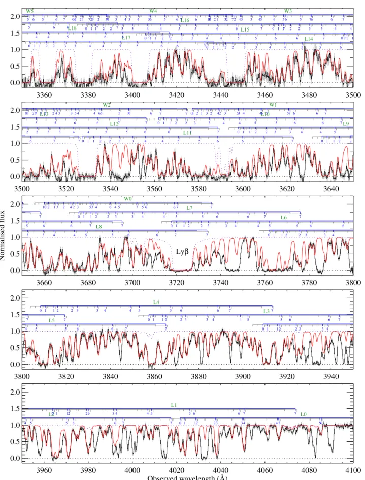
Bluewards of λobs = 4100 Å, the spectrum is crowded with

numerous H2lines from different rotational levels (Fig.10),

con-firming the detection fromNoterdaeme et al.(2019) based on a low-resolution, low-S/N BOSS spectrum. We modelled the H2

absorption profile using three components (which we label A, B, and C from blue to red). The strongest two components (B and C) are located close to each other in velocity space, so their respective absorption lines are strongly blended. Notwithstand-ing, these two components are also seen in the neutral chlorine profile (with total log N(Cl

_i

) ≈ 13.4 ± 0.1, see Fig.11), which is known to be chemically linked to H2(see e.g.,Balashev et al.

2015and references therein).

We first used standard multi-component fitting using vpfit, including rotational levels up to J = 5. Because of the decreas-ing S/N and increasing line blending towards the blue, only the data at λ > 3600 Å was used to constrain the fit of the molecu-lar hydrogen lines. We tied together the redshifts and Doppler parameters between rotational levels for a given component. This implicitly assumes that H2 in different rotational levels is

3360 3380 3400 3420 3440 3460 3480 3500 0.0 0.5 1.0 1.5 2.0 0 1 1 0 1 1 2 2 3 3 4 4 0 1 1 2 2 3 3 4 4 5 5 6 L14 0 1 1 2 2 3 3 4 4 5 5 6 6 7 7 L15 0 1 1 2 2 3 3 4 4 5 5 6 6 7 7 L16 0 1 1 2 2 3 3 4 4 5 5 6 6 7 7 L17 4 4 5 5 6 6 7 7 L18 5 6 6 7 7 10 2 1 32 2 43 3 45 4 5 6 5 76 6 7 W3 0 1 2 1 23 2 34 3 4 5 4 56 5 6 7 6 7 7 W4 5 6 5 6 7 6 7 7 W5 3500 3520 3540 3560 3580 3600 3620 3640 0.0 0.5 1.0 1.5 2.0 0 1 1 2 2 3 3 4 4 5 5 6 6 7 L10 0 1 1 2 2 3 3 4 4 5 5 6 6 7 7 L11 2 2 3 3 4 4 5 5 6 6 7 7 L12 5 5 6 6 7 7 L13 6 7 7 0 1 1 2 2 0 1 1 2 2 3 3 4 4 5 L9 01 2 1 3 2 42 3 53 4 46 5 57 6 6 7 W1 01 2 1 3 2 2 4 3 3 5 4 4 65 5 76 6 7 7 W2 7 3660 3680 3700 3720 3740 3760 3780 3800 0.0 0.5 1.0 1.5 2.0 Normalised flux 7 0 1 1 2 2 3 3 4 0 1 1 2 2 3 3 4 4 5 5 6 6 L6 0 1 1 2 2 3 3 4 4 5 5 6 6 7 7 L7 3 3 4 4 5 5 6 6 7 7 L8 5 6 6 7 7 10 2 1 3 2 4 2 3 53 4 6 4 5 7 5 6 6 7 7 W0 7 Lyβ 3800 3820 3840 3860 3880 3900 3920 3940 0.0 0.5 1.0 1.5 2.0 0 1 1 2 2 3 3 4 0 1 1 2 2 3 3 4 4 5 5 6 6 7 L3 0 1 1 2 2 3 3 4 4 5 5 6 6 7 7 L4 4 5 5 6 6 7 7 L5 7 7 3960 3980 4000 4020 4040 4060 4080 4100 Observed wavelength (Å) 0.0 0.5 1.0 1.5 2.0 0 1 12 23 34 4 5 56 L0 0 1 12 23 3 4 4 5 5 6 6 7 7 L1 4 5 5 6 6 7 7 L27

Fig. 10.Portion of X-shooter UVB spectrum of J0015+1842 (black, with uncertainties in grey). Horizontal blue segments connect rotational levels (short tick marks) from a given Lyman (L) or Werner (W) band of H2for the central H2component. The same is shown in grey for the two other

components, but they are not labelled for visibility. The overall model (MCMC-based) spectrum is over-plotted in red, with contribution from non-H2lines (H

i

and metal lines) shown as a dotted purple line.

−800 −600 −400 −200 0 200 Relative velocity (km s−1₎ 0.0 0.5 1.0 ClI λ1347

Fig. 11.Fit to neutral chlorine absorption line. The observed data are shown in black, with the best-fit profile shown in red. Top panel: resid-uals (black) and 1σ error level (orange). The short tick marks show the location of the H2components, while long dashed blue lines show those

of other metal lines. As for all similar figures in this work, the origin of the velocity scale is set to zref= 2.631.

well mixed, which is not necessarily the case. Indeed, an increase of b with J has been observed with VLT/UVES in a few cases of relatively low H2column densities (e.g.,Noterdaeme et al. 2007;

Balashev et al. 2009;Albornoz Vásquez et al. 2014). However, in this work, the fit to the lower rotational levels is independent of the exact b value since the lines are damped.

Given the complexity of the H2 absorption spectrum and

to account for the possibility of different Doppler parameters, which can have an effect on the high-J levels, we also fitted the H2lines with a Markov chain Monte Carlo (MCMC) procedure.

During this fit, we again tied the Doppler parameters of J = 0 and J = 1, as these levels are mostly co-spatial, but those from other rotational levels were allowed to vary independently. How-ever, we added a penalty function to the likelihood function to favour the solutions where Doppler parameters increase with J. We also included the H2absorption from J = 6 and J = 7

lev-els: these are albeit marginally detected. To get posteriors on fit-ting parameters, we used an affine sampler (Goodman & Weare 2010) with a flat prior on log N, b, and z. The result from the MCMC fit is shown in Fig.10, but we note that the standard vpfit procedure provides a visually almost indistinguishable profile. Indeed, higher spectral resolution remains necessary to ascertain the velocity structure and widths of the lines. Hence, we provide the best-fit parameters from both fitting methods in Table3.

In all three components, the column densities of high rota-tional levels (J & 2) are significantly enhanced compared to what is seen in typical H2-bearing DLAs at high redshifts. The

observed T01temperatures (∼100 K for components B and C and

closer to ∼200 K for component A) remain consistent with what is seen for intervening systems, albeit with a small tendency to be in the upper range for the observed column densities (e.g., Balashev et al. 2019). This could result from an enhanced heat-ing of the gas through photoelectric effect of UV photons on dust grains. We discuss the observed H2excitation diagrams

quanti-tatively in Sect.5.2. 4.3. Chemical enrichment

Metal absorption lines are seen spread over 600 km s−1mostly bluewards of the systemic redshift. Since the H

_i

column den-sity is large enough for self-shielding from ionising photons, we focused our analysis on the low-ionisation species in order to estimate the gas phase metallicity, since these are in their domi-nant ionisation stage in the neutral gas.

The initial guess for the velocity decomposition was obtained from the absorption lines of singly ionised silicon and iron that have several transitions with a wide range of oscillator strengths.

Singly ionised sulphur and zinc were subsequently added to the model, and finally, all parameters were fitted simultaneously under the usual assumption that Zn

_ii

, S

_ii

, Si

_ii

, and Fe

_ii

are located in the same gas (i.e. we tied their Doppler parameters and redshifts). Since Zn

_ii

λ2026 is blended with Mg

_i

λ2026, we also included this line in the fit with an independent Doppler parame-ter and redshift. We note that Si

_ii

λ1526 is detected in the overlap between the UVB and VIS spectra. We therefore included both these spectral regions to constrain the fit.

The result of the fits are shown in Fig. 12 and the corre-sponding parameters are provided in Table 4. The total col-umn densities are log N(cm−2_{) = 15.52 ± 0.03 (Si}

ii

), 14.46 ± 0.02 (Fe

_ii

), 15.39 ± 0.08 (S

_ii

), and 13.34 ± 0.07 (Zn

_ii

). Using the total H (H

_i

+ H2) column density, log N(H)= 20.75 ±

0.02, these values translate to overall gas-phase abundances of [Si/H] = −0.74 ± 0.04, [Fe/H] = −1.77 ± 0.03, [S/H] = −0.49 ± 0.08, and [Zn/H] = −0.39 ± 0.05, where ionisation corrections were assumed to be negligible, and the solar reference values were taken fromAsplund et al.(2009) following the recommen-dation ofLodders et al.(2009) on whether to use photospheric, meteoritic, or average values. Both zinc and sulphur are known to be volatile species and hence provide a good estimate of the metallicity, which is about 40% solar. In turn, silicon and iron tend to deplete more onto dust grains (e.g.,De Cia et al. 2016). Indeed, we measured depletion by a factor of two for silicon, while 96% of iron is locked into dust grains.

4.4. Excited carbon and silicon

Neutral carbon absorption lines are detected in the spectrum of J0015+1842. This is not surprising given the presence of H2 and the high metallicity of the system (Noterdaeme et al.

2018). Three components are detected, matching those seen in H2, and we detect all three fine structure levels of the ground

state triplet (2s2_2p2 3_P

J=0,1,2). All C

i

(J = 0), C

i

* (J = 1),

and C

_i

** (J = 2) lines were first fitted together using the bands at 1277, 1280, 1328, 1560, and 1656 Å, avoiding regions affected by blends (in particular for the 1328 Å band) and tying the redshifts and Doppler parameters for each component. The result of the fit is shown in Fig. 13, and the corresponding parameters are summarised in Table5. The Doppler parameters are found to be as small as 1 km s−1. While such small values are similar to what is seen in H2, and not uncommon for C

i

-absorbers (e.g.,Noterdaeme et al. 2017), here they are observed far below the spectral resolution, implying large uncertainties on the column densities. We therefore repeated the fit using the MCMC method, which suggested that the uncertainties on the b-values provided by vpfit were likely underestimated. Finally, we performed a final test assuming a fixed, somehow higher b = 3.5 km s−1 _{value. The column densities obtained from the}

different methods remain similar, although differing in some cases by up to ∼0.5 dex. Nevertheless, all results indicate higher excited-to-ground, fine-structure level ratios than usually seen in intervening systems. We caution, however, that high spectral resolution observations remain vital to accurately measuring the corresponding column densities.

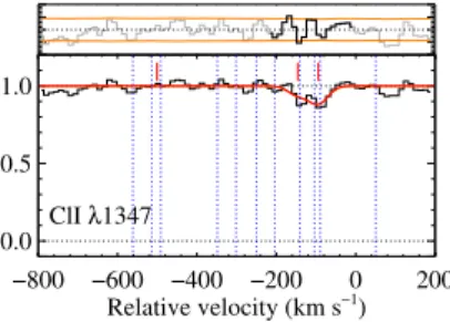
Singly ionised carbon and silicon are also detected in excited fine-structure states (C

_ii

* and Si

_ii

*, respectively). While C

_ii

* is in principle useful in estimating the cooling rate of the gas through [C

_ii

]158 µm emission (Pottasch et al. 1979), the corre-sponding absorption lines here are saturated, impeding the mea-surement of the C

_ii

* column density.

The Si

_ii

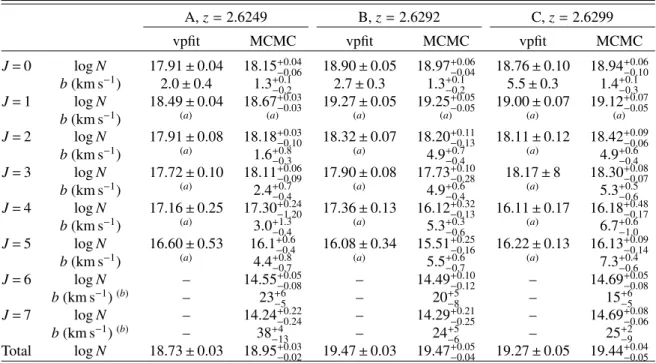
* absorption is in turn much weaker but clearly detected in its strongest line at 1264 Å. We identify three main

Table 3. Result of Voigt profile fitting to molecular hydrogen lines.

A, z= 2.6249 B, z= 2.6292 C, z= 2.6299

vpfit MCMC vpfit MCMC vpfit MCMC

J= 0 log N 17.91 ± 0.04 18.15+0.04_−0.06 18.90 ± 0.05 18.97+0.06_−0.04 18.76 ± 0.10 18.94+0.06_−0.10 b(km s−1) 2.0 ± 0.4 1.3+0.1_−0.2 2.7 ± 0.3 1.3+0.1_−0.2 5.5 ± 0.3 1.4+0.1_−0.3 J= 1 log N 18.49 ± 0.04 18.67+0.03_−0.03 19.27 ± 0.05 19.25+0.05_−0.05 19.00 ± 0.07 19.12+0.07_−0.05

b(km s−1₎ (a) (a) (a) (a) (a) (a)

J= 2 log N 17.91 ± 0.08 18.18+0.03_−0.10 18.32 ± 0.07 18.20+0.11_−0.13 18.11 ± 0.12 18.42+0.09_−0.06

b(km s−1) (a) 1.6+0.8_−0.3 (a) 4.9+0.7_−0.4 (a) 4.9+0.6_−0.4

J= 3 log N 17.72 ± 0.10 18.11+0.06_−0.09 17.90 ± 0.08 17.73+0.10_−0.28 18.17 ± 8 18.30+0.08_−0.07 b(km s−1₎ (a) _2.4+0.7 −0.4 (a) _4.9+0.6 −0.4 (a) _5.3+0.5 −0.6 J= 4 log N 17.16 ± 0.25 17.30+0.24_−1.20 17.36 ± 0.13 16.12+0.32_−0.13 16.11 ± 0.17 16.18+0.48_−0.17

b(km s−1) (a) 3.0+1.3_−0.4 (a) 5.3+0.3_−0.6 (a) 6.7+0.6_−1.0

J= 5 log N 16.60 ± 0.53 16.1+0.6_−0.4 16.08 ± 0.34 15.51+0.25_−0.16 16.22 ± 0.13 16.13+0.09_−0.14

b(km s−1) (a) 4.4+0.8_−0.7 (a) 5.5+0.6_−0.7 (a) 7.3+0.4_−0.6

J= 6 log N – 14.55+0.05_−0.08 – 14.49+0.10_−0.12 – 14.69+0.05_−0.08 b(km s−1₎(b) _{– 23}+6 −5 – 20+5−8 – 15+6−5 J= 7 log N – 14.24+0.22_−0.24 – 14.29+0.21_−0.25 – 14.69+0.08_−0.06 b(km s−1)(b) _{– 38}+4 −13 – 24+5−6 – 25+2−9 Total log N 18.73 ± 0.03 18.95+0.03_−0.02 19.47 ± 0.03 19.47+0.05_−0.04 19.27 ± 0.05 19.44+0.04_−0.05

Notes.(a)_{Doppler parameter tied for all rotational levels (vpfit) and for J= 0 and J = 1 (MCMC).}(b)_{The absorption lines corresponding to these}

levels are little sensitive on the Doppler parameter.

components that correspond to those seen in the metal lines. We also used the weaker 1309 Å line to ascertain the detection and constrain the fit, shown in Fig.14. The corresponding parameters are given in Table4.

4.5. Dust extinction

We fitted the dust reddening using the formalism by Fitzpatrick & Massa (2007) assuming various fixed extinction laws (Gordon et al. 2003) to identify the overall shape of the dust reddening law applied to the composite X-shooter spectrum from Selsing et al. (2016). The details of the method are pre-sented byNoterdaeme et al.(2017). We found a best match using a rather shallow extinction curve like the one observed towards the Large Magellanic super-shell (LMC2). However, we needed to vary the strength of the extinction bump at 2175 Å in order to properly match the observed spectrum. The spectrum exhibits significant variations of the iron emission lines in the region between the C

_iv

and Mg

_ii

lines. We included a model of these iron lines using the template given by Vestergaard & Wilkes (2001). While this template improves the overall fit, the exact variations of the myriad of iron lines cannot be captured by a fixed line template. Taking systematic uncertainties due to vari-ations in the intrinsic quasar shape into account, we found a best-fit solution of A(V) = 0.4 ± 0.1 mag, Fe2 = 0.5 ± 0.2,

Fe3 = −1.5 ± 0.5, c3 = 0.7 ± 0.1, where A(V) is the amount

of extinction and Fe2and Fe3multiplicative factors

parametris-ing the strengths of the Fe

_ii

and Fe

_iii

lines with respect to the template. The inferred strength of the 2175 Å bump is Abump =

πc3/(2γ) = 1.2 ± 0.2, where γ = 0.95 is the width of the bump

(Gordon et al. 2003). The best-fit solution is shown in Fig.15. Based on the inferred extinction law from the spectral fitting, we constructed a dust model to reproduce this extinction law by varying the dust-grain size distribution and the ratio of sil-icate to graphite grains (Si/C). The grain size distribution was

assumed to be a power-law distribution with a slope of −3.5 and a maximum grain size of 0.25 µm similar to the standard ISM size distribution (e.g.,Nozawa & Fukugita 2013). The best match to the extinction law was found for a minimum dust grain size of 0.01 µm (compared to 0.005 µm for standard ISM dust grains) and a silicate-to-graphite ratio of Si/C = 2 relative to the standard ISM abundance ratio.

5. Results and discussions

In this section, we first discuss the implications of the emis-sion line properties and why this suggests that we are observing galactic-scale outflows, and we show that the absorbing gas is likely a different manifestation of the same galactic-scale out-flows, intercepted by the line of sight to the nucleus. We then derive the physical conditions in the absorbing gas and its dis-tance to the central engine. Finally, we substantiate the overall picture by modelling the Ly-α absorption-emission profile both spatially and spectrally.

5.1. Evidence of galactic-scale outflows 5.1.1. The extended emission from ionised gas

According to the standard paradigm of AGN, the broad emis-sion lines of quasars arise from dense regions with high veloc-ities close to the central engine. Since these regions are far too small (∼1 pc, e.g.,Kaspi et al. 2007) to be resolved at cos-mological distances, information about their sizes is generally obtained through reverberation mapping (Blandford & McKee 1982). However, valuable constraints can also be obtained from partial coverage by a foreground absorber (e.g.,Balashev et al. 2011).

The narrow emission lines are in turn expected to arise fur-ther away from the obscuring torus, from gas at sufficiently low density where the emission is dominated by forbidden-line

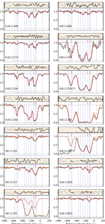
0.0 0.5 1.0 FeII λ1608 0.0 0.5 1.0 SiII λ1808 0.0 0.5 1.0 FeII λ2374 0.0 0.5 1.0 SiII λ1526 0.0 0.5 1.0 FeII λ2344 0.0 0.5 1.0 SiII λ1526UV 0.0 0.5 1.0 FeII λ2382 0.0 0.5 1.0 SiII λ1260 0.0 0.5 1.0 SII λ1250 0.0 0.5 1.0 SiII λ1304 0.0 0.5 1.0 SII λ1253 0.0 0.5 1.0 ZnII λ2026 −800 −600 −400 −200 0 200 Relative velocity (km s−1₎ 0.0 0.5 1.0 SII λ1259 −800 −600 −400 −200 0 200 Relative velocity (km s−1₎ 0.0 0.5 1.0 ZnII λ2062

Fig. 12.Fit to metal absorption lines. The observed data are shown in black with the synthetic profile for each given species overplotted in red. In case of several lines contributing to the observed profile (see e.g., S

_ii

λ1259 and Si

_ii

λ1260), the contribution for the labelled line alone is shown in red, while the total synthetic profile is shown in orange. Resid-uals are shown in the small panel above each line, with the orange line showing the 1σ error level. The location of the different components of the model are indicated by blue vertical dashed lines, with short red marks showing the position of H2components. The zero of the velocity

scale is set to zref= 2.631.

transitions. While initially thought to be less than kpc-sized, evi-dence of the presence of extended narrow line regions (NLR) around diverse types of AGN has increased. This is particularly evident for low redshift Type 2 AGN, where the observations are facilitated by larger angular sizes and obscuration of the nucleus

emission (e.g.,Sun et al. 2017). However, evidence for kpc-scale emission is also seen in high-redshift quasars (e.g.,Rupke et al. 2017). This also includes the ubiquity of giant (&100 kpc) Lyα nebulae around luminous quasars at 3 < z < 4 (Borisova et al. 2016). The narrow emission lines therefore contain important information for the study of ionised gas on large scales.

If the energy from accretion disc winds propagates to the host galaxy ISM, then we expect to observe some connection between the properties of the different types of emission lines. For exam-ple, Coatman et al.(2019) observed a correlation between the blueshifts of the overall C

_iv

and [O

_iii

] emissions, as well as an anti-correlation between [O

_iii

] equivalent width and C

_iv

blueshift. This suggests that high-velocity accretion disc winds, arising in a compact region very close (<1 pc) to the supermas-sive black hole (Netzer 2015) can influence the host-galaxy on kpc-scales, assuming [O

_iii

] is extended over such scales2_{. While}

our observation here concerns a single object, the observed kinematics and equivalent width are in agreement with those observed by these authors. More importantly, we also confirm that most of the C

_iv

emission arises from the broad nuclear region, but we observe a weak C

_iv

emission at least as extended as the narrow [O

_iii

] emission, supporting the above picture. Finally,Tombesi et al.(2015) found evidence for accretion-disc winds driving galactic-scale molecular outflows, as later con-firmed by Veilleux et al. (2017). Taken together, these works suggest that the H2 absorption system observed here could be

linked to the same outflow process.

The commonly-used Baldwin et al. (1981, BPT) diagram provides a useful diagnostic to discriminate between photoioni-sation by AGN or star formation. While we do not have access to the [N

_ii

] or Hα lines, the fact that [O

_iii

] is detected outside the unresolved nuclear region while Hβ is not (see Figs.3and5) suggests a very high [O

_iii

]/Hβ ratio, as expected in the case of ionisation by AGN (e.g., Kewley et al. 2001; Kauffmann et al. 2003). This ionisation mechanism is further supported by the large velocity dispersion, FWHM ∼ 600 km s−1, of the extended [O

_iii

] emission (see e.g.,Zhang & Hao 2018).

As shown in Sect.3.4, the narrow [O

_iii

] emission presents two blobs on both sides of the nucleus (at a distance of ∼5 kpc projected on the plane of the sky) and with opposite line-of-sight velocities with respect to our reference redshift. The bulk veloc-ities of the emission are of several hundred km s−1. These are at the limit between what is expected from rotational and non-gravitational velocities (e.g.,Comerford et al. 2018). However, the emission is well detached from the nucleus (in particular the red lobe, see Fig.7) which is better explained by an outflow. This is also consistent with the presence of blueshifted broad [O

_iii

] emission closer to the nucleus, following the picture of energy propagation from the inner to the outer regions (e.g., Fabian 2012). Since the [O

_iii

] emissivity scales with the square of the density, the observed [O

_iii

] emission traces the densest ionised gas clouds, which, being detached, could indicate com-pressed regions at the front of the outflow. Furthermore, a careful look at Fig.6reveals that as the distance from the nuclear emis-sion increases, the line width of the narrow emisemis-sion decreases, and the centroid of the emission approaches the systemic veloc-ity (see right panels of that figure). These kinematic signatures are consistent with a decelerating outflow and a possible com-pression at the front of the outflow. However, this interpreta-tion remains tentative and requires confirmainterpreta-tion through deeper

2 _{This was actually not constrained by the data obtained by}

Table 4. Result of Voigt profile fitting to singly ionised metal lines. z b(km s−1_{) log N(cm}−2₎ Si

_ii

Fe

_ii

S

_ii

Zn

_ii

Si

_ii

* 2.624197 6.6 ± 2.2 13.30 ± 0.13 – – – – 2.624772 13.1 ± 1.4 14.41 ± 0.10 13.32 ± 0.03 14.48 ± 0.05 11.81 ± 0.20 11.81 ± 0.27 2.625051 58.9 ± 3.2 13.83 ± 0.05 12.88 ± 0.08 – – – 2.626781 12.3 ± 1.6 13.98 ± 0.10 13.10 ± 0.06 – – – 2.627347 24.6 ± 4.9 14.48 ± 0.04 13.34 ± 0.05 14.32 ± 0.11 – 12.66 ± 0.05 2.627968 12.4 ± 0.9 14.99 ± 0.05 13.89 ± 0.02 14.66 ± 0.07 12.25 ± 0.06 12.97 ± 0.06 2.628528 14.7 ± 1.1 14.37 ± 0.04 13.44 ± 0.02 13.81 ± 0.28 10.84 ± 1.44 11.49 ± 0.67 2.629299 14.9 ± 1.2 14.52 ± 0.08 13.82 ± 0.04 14.65 ± 0.08 12.27 ± 0.08 12.44 ± 0.09 2.629742 5.1 ± 1.2 14.59 ± 0.15 13.63 ± 0.07 14.99 ± 0.20 12.73 ± 0.08 12.62 ± 0.32 2.629918 32.3 ± 2.2 14.76 ± 0.07 – – – – 2.631610 24.5 ± 1.1 13.64 ± 0.02 12.95 ± 0.03 – – – Total 15.52 ± 0.03 14.46 ± 0.02 15.39 ± 0.08 12.99 ± 0.05 13.34 ± 0.07 6000 6005 6010 6015 6020 6025 Observed wavelength (Å) 0.2 0.4 0.6 0.8 1.0 1.2 Norm. flux _CIλ1656 J=2 J=1 J=0 −0.10.0 0.1 5650 5655 5660 5665 5670 5675 Observed wavelength (Å) 0.4 0.5 0.6 0.7 0.8 0.9 1.0 1.1 Norm. flux _CIλ1560 J=2 J=1 J=0 −0.10.0 0.1 4810 4815 4820 4825 4830 4835 Observed wavelength (Å) 0.4 0.5 0.6 0.7 0.8 0.9 1.0 1.1 Norm. flux _CIλ1328 J=2 J=1 J=0 −0.10.0 0.1 4620 4625 4630 4635 4640 4645 4650 4655 Observed wavelength (Å) 0.4 0.5 0.6 0.7 0.8 0.9 1.0 1.1 Norm. flux _{CIλ1277 1280} J=2 J=1 J=0 −0.10.0 0.1

Fig. 13.Fit to C

i

absorption lines. The data are shown in black with the best-fit over-plotted in red. The contribution from individual fine-structure levels are shown in orange (C

_i

), green (C

_i

*), and purple (C

_i

**). Top panels: residuals.

observations with higher spatial resolution, ideally using integral field spectroscopy.

5.1.2. Kinematics: Absorption and emission as different manifestations of the same wind

While the velocity profile of neutral hydrogen seen in absorp-tion is not directly accessible because of saturaabsorp-tion of H

_i

lines, from Fig. 16 it is clear that the profiles of low-ionisation and high-ionisation metal species share the same overall structure, with several components spread over about 600 km s−1, almost completely blueshifted with respect to the assumed systemic redshift. Such a broad, blueshifted structure is consistent with the expected signature of outflowing gas. The kinematics con-trast what is usually seen in intervening DLAs, where the veloc-ity spread of low-ionisation metals are generally much smaller (Ledoux et al. 2006) and systematically less extended than more ionised species (see Fig. 4 of Fox et al. 2007). The profiles observed here suggest that ionised and neutral phases could be well mixed up within the gross structure of the outflowing gas.

The absorption line kinematics observed in the spectrum of J0015+1842 also corresponds well to the kinematics of the blueshifted, extended, ionised gas seen in emission (the blue component of the extended [O

_iii

] emission), indicating that we are looking at the same phenomenon both in emission and absorption and that the kpc-scale outflowing gas likely contains a mixture of different phases. A similar interpretation has recently been put forward byXu et al.(2020). Based on the kinematics of [O

_iii

] emission and C

_iv

absorption in seven quasars, the authors suggest that outflows seen in emission and absorption are likely different manifestations of the same wind.

5.2. Physical conditions in the absorbing gas

If the absorbing gas is also part of the outflow, which can typ-ically span around a few tens of kpc from the AGN, then we expect to see effects of the quasar proximity on the physical conditions. The presence and excitation of atomic and molec-ular species provides a unique opportunity to investigate these physical conditions.

Singly-ionised silicon is an interesting species since its excited fine-structure level has been detected in only a few high-z intervening DLAs to date (e.g., Kulkarni et al. 2012; Noterdaeme et al. 2015) and most likely in regions of high

Table 5. Result of Voigt profile fitting to neutral carbon lines. z b(km s−1_{) log N(cm}−2₎ C

i

, J= 0 C

i

, J= 1 C

i

, J= 2 vpfit, free b 2.62484 0.9 ± 0.5 12.82 ± 0.43 13.39 ± 0.29 12.45 ± 0.48 2.62919 1.3 ± 0.2 13.47 ± 0.28 14.06 ± 0.19 13.13 ± 0.20 2.62973 3.6 ± 0.4 13.41 ± 0.11 14.05 ± 0.07 13.93 ± 0.07 MCMC, free b 2.62482 1.7+2.0_−0.7 12.82+0.30_−0.35 13.30+0.10_−0.14 12.72+0.27_−0.65 2.62914 2.3+7.0_−1.0 13.11+0.15_−0.15 13.50+0.08_−0.09 13.07+0.16_−0.13 2.62973 2.3+0.3_−0.3 13.75+0.34_−0.26 14.66+0.30_−0.15 14.27+0.18_−0.18 vpfit, fixed b 2.62483 3.50 12.59 ± 0.30 13.15 ± 0.10 12.22 ± 0.72 2.62914 3.50 13.15 ± 0.13 13.54 ± 0.08 13.03 ± 0.15 2.62972 3.50 13.44 ± 0.11 14.15 ± 0.07 13.96 ± 0.07

pressure (Neeleman et al. 2015). However, it appears to be more conspicuous in proximate DLAs, where the excitation of sil-icon fine structure could be enhanced by both high densities and strong UV flux (e.g.,Ellison et al. 2010;Fathivavsari et al. 2018). Hence, its presence may indicate close proximity to the quasar central engine. However, in the absence of other informa-tion, it is hard to discriminate between the case of high density or high UV flux.

Molecular hydrogen can provide important information, since both the presence of H2and the excitation of its rotational

levels depend on the strength of the UV field, the gas density and its temperature (e.g., Balashev et al. 2019). Owing to for-mation on dust grains and destruction through line absorption in the Lyman and Werner bands, the presence of molecular hydro-gen mainly depends on the ratio between the UV intensity and the gas density (e.g.,Sternberg et al. 2014). This implies that the density required for an atomic-to-molecular transition to occur follows n ∝ d−2_{, where d is the distance to the central UV source.}

For the H

_i

column density and metallicity (or equivalently dust-to-gas ratio) observed for J0015+1842, the normalisation of this relation3_{is about log n (cm}−3_{) ∼ 4 at d ∼ 10 kpc distances from}

the nucleus (Noterdaeme et al. 2019).

Combining the information from Si

_ii

* and H2, as well as

other species sensitive to the density and UV radiation (e.g., C

_i

fine structure, whether CO molecules are present or not), can therefore provide constraints on the physical state of the gas and its distance to the central UV source. In Fig.17, we compare the apparent optical depths of the Si

_ii

λ1808 and Si

_ii

*λ1264 lines4_,

which are both optically thin. The ground state and excited pro-files of singly-ionised silicon have similar velocity propro-files with three main clumps, two of which coincide with the positions of H2 absorption components. Yet, the strongest bulk

compo-nent of Si

_ii

* does not align with the H2components. In the top

panel of Fig.17, we show the ratio of Si

_ii

*/Si

_ii

. This ratio is not enhanced at the position of H2 absorption, where instead it

tends to be consistently lower than average over several pixels. Since molecular hydrogen traces the high-density regions in the absorbing gas, this may suggest that the high excitation of Si

_ii

* is not due to high density but rather due to strong UV irradiation. 3 _{We note that this simple estimate assumes the transition to occur and}

does not exclude the presence of H2at lower densities (or distances) if

the transition is not complete.

4 _{We caution that Si}

ii

*λ1264 is partly blended with Si

_ii

*λ1265. How-ever, the latter has an oscillator strength ten times smaller than the for-mer, so the impact on the apparent optical depth remains small.

−800 −600 −400 −200 0 200 Relative velocity (km s−1₎ 0.0 0.5 1.0 SiII* λ1264 −800 −600 −400 −200 0 200 Relative velocity (km s−1₎ 0.0 0.5 1.0 SiII* λ1309

Fig. 14.Same as Fig. 12 for the absorption lines from excited fine-structure of singly-ionised silicon.

5.2.1. Modelling warm and cold gas as successive slabs Since the quasar itself is likely the dominant source of pho-tons striking the medium at distances . few tens of kpc, the UV field received by each slab of gas (absorption component) actually depends on the transmitted field through the previous slab of gas on the line of sight. While understanding succes-sive filtering slabs of gas makes the study of proximate systems significantly more complex than intervening ones (where the components can generally be treated independently), advantages are that the observed column densities correspond to the actual layers through which UV photons propagate, and we have prior knowledge about the shape of this field5_{. However, the large}

number of components and their unknown respective physical locations along the line of sight does not allow for a full mod-elling of the system, which would have far too many parameters to vary.

We simplified the problem by considering two successive slabs of gas along the line of sight to get an idea of the physi-cal conditions in the different phases. In this picture, one slab of warm gas, directly illuminated by the quasar, is likely responsi-ble for most of the Si

_ii

*, while the second slab, for which the incident field contains no more H-ionising photons, is in a cold state and contains the H2.

We used the photoionisation code Cloudy v17.1 (Ferland et al. 2017), running grids of constant density models with plane-parallel geometry illuminated on one side by the built-in cloudy AGN spectral energy distribution. The cosmic microwave and cosmic ray backgrounds were included. The gas phase abundances were set to match the observed ones, and we included dust using the grain mixture and size distri-bution described in Sect. 4.5. In the first runs, the abundance of dust was scaled to self-consistently (i.e. conserving mass) match the observed depletion factors of iron and silicon. This in turn implies depletion factors of about 50% and 25% for carbon and oxygen, respectively. We tested and found that the results concerning the first layer are actually little sensitive to the abundance of dust, except, naturally, for the calculated extinction, which tends to strongly exceed the observed one due to the large total column density in the model. However, as we see below, the first layer contains mostly ionised gas, as well as neutral gas with high temperatures (>104K), so it is most likely that grains, in particular small ones, are destroyed. We then assumed no grains in that phase – but these are kept in the second (cold) slab.

The results concerning the excitation of silicon in the first slab are shown in Fig.18, where the UV flux is converted into 5 _{In turn, modelling of intervening DLAs is generally intended to}

reproduce the observed column densities, but the actual incident flux intensity and shape is not known (for example, whether it is attenuated or not before striking the cloud) and there is no reason for its direction to match that of the line of sight.