HAL Id: cea-01004466
https://hal-cea.archives-ouvertes.fr/cea-01004466
Submitted on 3 Nov 2020
HAL is a multi-disciplinary open access
archive for the deposit and dissemination of
sci-entific research documents, whether they are
pub-lished or not. The documents may come from
teaching and research institutions in France or
abroad, or from public or private research centers.
L’archive ouverte pluridisciplinaire HAL, est
destinée au dépôt et à la diffusion de documents
scientifiques de niveau recherche, publiés ou non,
émanant des établissements d’enseignement et de
recherche français ou étrangers, des laboratoires
publics ou privés.
multicolour photometry
C. Maraston, J. Pforr, A. Renzini, Emanuele Daddi, M. Dickinson, Alessandro
Cimatti, C. Tonini
To cite this version:
C. Maraston, J. Pforr, A. Renzini, Emanuele Daddi, M. Dickinson, et al.. Star formation rates and
masses of z
2 galaxies from multicolour photometry. Monthly Notices of the Royal Astronomical
Society, Oxford University Press (OUP): Policy P - Oxford Open Option A, 2010, 407, pp.830-845.
�10.1111/j.1365-2966.2010.16973.x�. �cea-01004466�
arXiv:1004.4546v1 [astro-ph.CO] 26 Apr 2010
Star formation rates and masses of z ∼ 2 galaxies from
multicolour photometry
Claudia Maraston
1⋆, Janine Pforr
1, Alvio Renzini
2, Emanuele Daddi
3,
Mark Dickinson
4, Andrea Cimatti
5, Chiara Tonini
11Institute of Cosmology and Gravitation, University of Portsmouth, Dennis Sciama Building, Burnaby Road, PO1 3FX Portsmouth, UK 2INAF-Osservatorio Astronomico di Padova,Vicolo dell’Osservatorio 5, I-35122 Padova, Italy
3CEA, Irfu/SAp, F-91191 Gif-sur-Yvette, France, France
4National Optical Astronomical Observatory, 950 N. Cherry Avenue, Tucson, AZ 85719, USA 5Dipartimento di Astronomia, Universit`a di Bologna, Via Ranzani, I-40126 Bologna, Italy
in press
ABSTRACT
Fitting synthetic spectral energy distributions (SED) to the multi-band photometry of galaxies to derive their star formation rates (SFR), stellar masses, ages, etc. requires making a priori assumptions about their star formation histories (SFH). A widely adopted parameterization of the SFH, the so-called τ -models where SFR ∝ e−t/τ
is shown to lead to unrealistically low ages when applied to a sample of actively star forming galaxies at z ∼ 2, a problem shared by other SFHs when the age is left as a free parameter in the fitting procedure. This happens because the SED of such galaxies, at all wavelengths, is dominated by their youngest stellar populations, which outshine the older ones. Thus, the SED of such galaxies conveys little information on the beginning of star formation, i.e., on the age of their oldest stellar populations. To cope with this problem, besides τ -models (hereafter called direct-τ models), we explore a variety of SFHs, such as constant SFR and inverted-τ models (with SFR ∝ e+t/τ), along with
various priors on age, including assuming that star formation started at high redshift in all the galaxies in the test sample. We find that inverted-τ models with such latter assumption give SFRs and extinctions in excellent agreement with the values derived using only the UV part of the SED, which is the one most sensitive to ongoing star formation and reddening. These models are also shown to accurately recover the SFRs and masses of mock galaxies at z ∼ 2 constructed from semi-analytic models, which we use as a further test. All other explored SFH templates do not fulfil these two test as well as inverted-τ models do. In particular, direct-τ models with unconstrained age in the fitting procedure overstimate SFRs and underestimate stellar mass, and would exacerbate an apparent mismatch between the cosmic evolution of the volume densities of SFR and stellar mass. We conclude that for high-redshift star forming galaxies an exponentially increasing SFR with a high formation redshift is preferable to other forms of the SFH so far adopted in the literature.
Key words: galaxies: evolution — galaxies: starbursts — galaxies: high-redshift
1 INTRODUCTION
The evolution of the baryonic component in galaxies is the hardest part to model in galaxy formation theories. How gas is accreted onto dark matter halos, its thermal history, how it is turned into stars, and if, how and when such star for-mation is quenched cannot be reliably predicted from first
⋆ E-mail: claudia.maraston@port.ac.uk
principles. The physical processes that are involved are too complex and non linear, with hydrodynamic simulations fail-ing by a large margin to cover the extremely wide dynamical range that would be required to describe phenomena rang-ing from the formation of stars and supermassive black holes to the behaviour of multiphase gas on megaparsec scales. Where it is hard to progress with pure theory alone, obser-vations can help and lead to further advances in our un-derstanding of how galaxies form and evolve. Indeed, over the last two decades a wealth of multiwavelength
observa-tions from both ground and space facilities have provided us with a rich vision of the galaxy populations in the high red-shift universe. Once correctly interpreted, such photometric, spectroscopic, and high spatial resolution data can provide
us with estimates of stellar mass (M∗), star formation rate
(SFR) and star formation history (SFH), structure, dynam-ics and nuclear activity, for a very large number of galaxies, and do so as a function of redshift and environment.
In particular, the accurate measurement of stellar mass and SFR is critical for trying to establish the evolution-ary links connecting galaxy populations at one redshift with those at another redshift. Setting constraints on the previous SFH of individual galaxies is also relevant in this context. All this is currently obtained by fitting the spectral energy dis-tribution (SED) of synthetic stellar populations to the SED of galaxies from their multi-band photometry. In practice, a large set of template synthetic SEDs is constructed with different SFHs, extinctions and metallicities, and a best fit
is sought by picking the SFH that minimises the χ2
r.
In this paper we focus on star forming galaxies at
1.4∼< z∼< 2.5, hence covering the epoch of major star
for-mation activity, and explore a wide set of SFHs showing ad-vantages and disadad-vantages of different parameterizations of
them. The case of passively evolving galaxies at z∼> 1.4 was
already addressed in Maraston et al. (2006).
It is well known that at z ∼ 2 galaxies with SFRs as
high as a few ∼ 100M⊙/yr−1are quite common (e.g., Daddi
et al. 2005), and by analogy with the rare objects at z ≃ 0 with similar SFRs (like Ultra Luminous Infra-Red Galaxies, ULIRGs), it was widely believed that such galaxies were caught in a merging-driven starburst. However, integral-field near-infrared spectroscopy has revealed that at least some of these galaxies have ordered, rotating velocity fields with no kinematic evidence for ongoing merging (Genzel et al. 2006). Still, the disk was shown to harbour several star-forming clumps and to have high velocity dispersion and gas fraction. All this makes such disk quite different from local disk galaxies, and it is now well documented that the same properties apply to many similar objects at z ∼ 2
(F¨orster-Schreiber et al. 2009).
That high SFRs in z ∼ 2 galaxies do not necessarily im-ply starburst activity became clear from a study of galaxies in the GOODS fields (Daddi et al. 2007a). Indeed, for
star-forming galaxies at 1.4∼< z∼< 2.5 the SFR tightly correlates
with stellar mass (with SFR ∝ ∼ M∗), with small
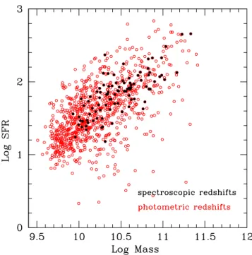
disper-sion (∼ 0.3 dex), as shown in Figure 1. Only a few galaxies lie far away from the correlation: a relatively small number of passive galaxies (with undetectable SFR, not shown in the figure), and sub-mm galaxies (SMG) with much higher SFRs, which may indeed be the result of gas-rich major mergers. Among starforming galaxies, the small dispersion
of the SFR for given M∗ demonstrates that these objects
cannot have been caught in a special, starburst moment of their existence. Rather, they must sustain such high SFRs for a major fraction of the time interval between z = 2.5 and z = 1.4, i.e. for some 1 − 2 Gyr, instead of the order of
one dynamical time (∼ 108 yr) typical of starbursts. Similar
correlations have also been found at lower redshifts, notably at z ∼ 1 (Elbaz et al. 2007), 0.2 ∼ z ∼ 1 (Noeske et al. 2007), and z ∼ 0 (Brinchmann et al. 2004).
In a recent study, Pannella et al. (2009) have measured
the average SFR vs. stellar mass for 1.4∼< z∼< 2.5 galaxies
Figure 1.The SFR vs. stellar mass of star forming BzK-selected galaxies in the GOODS-South field (from Daddi et al. 2007a). The sub-sample with spectroscopic redshifts is indicated, and repre-sents the set of galaxies for which various SED fits are attempted in this paper. The SFRs are in M⊙/yr and masses in M⊙units.
using the 1.4 GHz flux from the VLA coverage of the COS-MOS field (Schinnerer et al. 2007). When combined also with data at lower redshifts (see references above), Pannella et al. derive the following relation for the average SFR as a function of galaxy mass and time:
< SFR >≃ 270 × (M∗/1011M⊙) × (t/3.4 × 109yr)−2.5, (1)
where the SFR is in M⊙/yr units and t is the cosmic time,
i.e., the time since the Big Bang. Beyond z ∼ 2.5 (t∼< 2.7
Gyr) the specific SFR (= SFR/M∗) appears to flatten out
and remain constant all the way to very high redshifts (Daddi et al. 2009; Stark et al. 2009; Gonzalez et al. 2009). In parallel with these observational evidences, theorists are shifting their interests from (major) mergers as the main mechanism to grow galaxies, to continuous cold stream ac-cretion of baryons, that are then turned into stars in a quasi-steady fashion (e.g., Dekel et al. 2009). Clearly, a continuous, albeit fluctuating SFR such as in these cold stream models
provides a far better match to the observed tight SFR−M∗
relation, compared to a scenario in which star formation proceeds through a series of short starbursts interleaved by long periods of reduced activity. This is not to say that ma-jor mergers do not play a role. They certainly exist, and can lead to real giant starbursts bringing galaxies to SFRs as
high as ∼ 1000 M⊙/yr, currently identified with SMGs (e.g.
Tacconi et al. 2008; Menendez-Delmestre et al. 2009). Deriving SFRs, ages, stellar masses, etc. from SED fit-ting requires making assumptions on the previous SFH of galaxies. A widespread approach is to fit the SED of galax-ies at low as well as high redshifts with so called “τ -models”, i.e., synthetic SEDs in which the SFH is described by an
SFR = Ae−(t−t◦)/τ, (2)
where A =SFR(t = t◦). For a galaxy at cosmic time t a χ2
fit then gives the age (i.e., t − t◦, the time elapsed since the
beginning of star formation), the SFR e-folding time τ , the reddening E(B −V ), the metallicity Z and finally the stellar
mass M∗via the scale factor A. The SFR then follows from
Equation (2), where t is the cosmic time corresponding to the observed redshift of each galaxy. Of course, the reliability of the results depends on the extent to which the actual SFH is well represented by a declining exponential.
It is worth recalling that the first applications of τ -models were to figure out the ages of local elliptical galaxies, and the typical result was that the age is of the order of one Hubble time, and τ of the order of 1 Gyr or less (e.g., Bruzual 1983). This approach confirmed that the bulk of stars in local ellipticals are very old, hence formed within a short time interval compared to the present Hubble time. Later, the usage of τ -models was widely extended also to ac-tively star forming galaxies at virtually all redshifts, to the extent that it became the default assumption in this kind of studies (e.g., Papovich et al. 2001; Shapley et al. 2005;
Lee et al. 2009; Pozzetti et al. 2009; F¨oster-Schreiber et al.
2009; Wuyts et al. 2009b). Such an assumed SFH may give reasonable results for local spirals, as their SF activity has been secularly declining for an order of one Hubble time (e.g., Kennicutt 1986), but we shall argue that it may be a rather poor representation of the SFH of high-z galaxies, and may lead to quite unphysical results.
Cimatti et al. (2008) noted that the age of elliptical galaxies at z ∼ 1.6 turns out to be ∼ 1 Gyr both when using only the rest-frame UV part of the SED, and when using the whole optical-to-near-IR SED in conjunction with τ -models. However, they also noted that the former “age” is actually the age of the population formed in the last sig-nificant episode of star formation, while the latter “age” corresponds to the time elapsed since the beginning of star formation. The near equality of these two ages suggests that the SFR peaked shortly before being quenched, rather than having peaked at an earlier time and having declined ever since. Moreover, using τ models one implicitly assumes that galaxies are all caught at their minimum SFR, which is pos-sibly justified for local ellipticals and spirals, but not nec-essarily for star-forming galaxies at high redshifts that may actually be at the peak of their SF activity.
Indeed, an integration of dM∗/dt =< SFR > where
< SFR > is given by Equation (1) shows that the SFR can increase quasi-exponentially with time before the effect
of the declining term t−2.5 takes over, or star formation is
suddenly quenched and the galaxy turns passive (Renzini 2009). Mass and SFR formally increase exponentially when
SFR ∝∼ M∗, independent of time, as appears to be the case
for z∼> 2.5 (Gonzales et al. 2010). Thus, the observations of
both passive and star-forming galaxies at 1.4∼< z∼< 2.5
sug-gest that the SFRs of these galaxies may well have increased with time, rather than decreased. For these reasons, in this paper we use both direct-τ models, with the SFR given by Equation (2), as well as inverted-τ models in which the SFR increases exponentially with time, i.e.:
SFR = Ae+(t−t◦)/τ. (3)
Thus, direct-τ models assume that galaxies are caught
at their minimum SFR and had their maximum SFR at the beginning, whereas inverted-τ models assume that galaxies are caught at their maximum SFR and had their minimum SFR at the beginning. These two extreme assumptions may to some extent bracket the actual SFHs of real galaxies, or at least of the majority of them which, because of the tight
SFR−M∗relation, must have a relatively smooth SFH. Here
we explore which of the two assumptions gives the better fit to the SED of z ∼ 2 galaxies, and discuss the astrophysical plausibility of the relative results. Besides these exponen-tial SFHs we also consider the case of constant SFRs. In principle, other, differently motivated SFHs could also be explored, but in this paper we restrict the comparison to these three simple options, with SFRs increasing with time, decreasing, or constant.
The paper is organised as follows. Section 2 provides information on the galaxy data base that is used for our SED fitting experiments. Section 3 illustrates the procedure of SED fitting and describes the models. Section 4 presents the results we obtain for the different star formation history templates and their comparisons. Section 5 is devoted to a general discussion and presents our conclusions.
Finally, we adopt a cosmology with ΩΛ, ΩM and
h = H0/(100 kms−1Mpc−1) equal to 0.7, 0.3 and 0.75,
respectively, for consistency with most previous works. The age of the best-fit model is required to be lower than the age of the Universe at the given spectroscopic redshift. The SFR
and masses are always in M⊙/yr and M⊙units, respectively.
2 GALAXY DATA
We use a sample of 96 galaxies in the GOODS-South field from Daddi et al. (2007a). These galaxies were selected via the BzK diagram (Daddi et al. 2004) to be star forming, as confirmed by the detection in deep Spitzer+MIPS data at 24µm for > 90% of the galaxies in the sample. We in-clude only objects with accurately determined spectroscopic redshifts at z > 1.4, which were derived from a variety of surveys (see Daddi et al. 2007a for references), including
no-tably ultra-deep spectroscopy from the GMASS project1(J.
Kurk et al. 2009, in preparation) and from the GOODS survey at the Very large Telescope (Vanzella et al. 2008; Popesso et al. 2009). Galaxies in the resulting sample lie in the range 1.4 6 z 6 2.9.
The multicolour photometry was obtained using the 4 bands HST+ACS data in the optical (Giavalisco et al. 2004), the JHK bands in the near-IR from VLT+ISAAC observa-tions (Retzlaff et al. 2010) and from Spitzer+IRAC (Dick-inson et al., in preparation). We used PSF-matched images to build photometric catalogues from B to K. The IRAC
photometry was measured over 4′′ diameter apertures and
corrected to total magnitudes using corrections appropriate for point sources, and matched to the K band using to-tal K-band magnitudes as a comparison. This is the same procedure that was used for the GOODS-S catalogues pre-sented by Cimatti et al. (2008) and Daddi et al. (2007a). In summary, all SED fits make use of the following bands: BV izJHK plus the Spitzer/IRAC channels 1, 2 and 3.
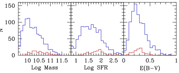
Besides satisfying the BzK criterion, the sample of galaxies used in this paper is subject to the additional selec-tion imposed by the various spectroscopic surveys menselec-tioned above. Figure 2 shows the distribution functions of the mass, SFR, and reddening, as derived by Daddi et al. (2007a),
sep-arately for the full KVega< 22 sample in the GOODS-South
field, and for the sub-sample of 96 objects with spectroscopic redshifts. The sample used here is somewhat biased towards higher masses, SFRs, and extinctions, but by and large for all three quantities it covers a major fraction of the range exhibited by the full sample. This can also be appreciated by inspecting Figure 1, where the 96 galaxies used in the present study are compared to the whole sample in Daddi et al. (2007a). Therefore, we consider that the conclusions drawn from this spectroscopic sample should hold for the full sample, perhaps with the exclusion of some low mass, low SFR objects.
This database allows the sampling of galaxy SEDs up to the rest-frame K band. The SEDs over the whole wave-length range from the rest-frame U V to the K band will be analysed in the next Sections.
3 SED FITTING
3.1 Generalities
The method we adopt for the SED fitting is similar to the one used in Maraston et al. (2006). We construct composite population templates based on the stellar population models of Maraston (2005) and we use an adapted version of the code Hyper-Z (Bolzonella et al. 2000), in which the SED
fitting is performed at fixed spectroscopic redshift2. We use
an updated version of Hyper-Z, kindly provided to us by M. Bolzonella, in which 221 ages (or τ ’s) are used for each kind of SFH, instead of the 51 used in earlier versions. The use of denser grids tends to give somewhat different results, an effect that is explored in detail in a parallel paper (J. Pforr et al. in preparation).
It is important to note that the code does not interpo-late on the tempinterpo-late grids, hence the tempinterpo-late set must be densely populated.
The fitting procedure is based on maximum-likelihood algorithms and the goodness of the fit is quantified via the
χ2r statistics. The code computes χ2r for a large number of
templates, which differ for SFHs, and finds the best-fitting template among them, having the reddening E(B −V ) as an additional free parameter. It is important to note that the code does not interpolate on the template grids, hence the
template set must be densely populated. The extinction AV
is allowed to vary from 0 to 3 in steps of 0.2, which corre-sponds to E(B − V ) from 0 to 0.74 according to the redden-ing law of Calzetti et al. (2000), that we adopt for all fits. By doing so we implicitly assume that the dust composition is the same in all examined galaxies and that there are no ma-jor galaxy to galaxy differences in the relative distribution of dust and young, hot stars. Differences in the extinction curve have been detected among z ∼ 2 galaxies, with some
2 For the fitting procedure we use photometric errors of 0.05 if
the formal error is smaller than that, to account for systematics in photometry and colour matching
galaxies exhibiting the 2175 ˚A UV bump, while others not
showing it (Noll et al. 2009), but such differences appear to have only minor effects on the derived SFR. Extinction is unlikely to be uniform across the surface of galaxies, partic-ularly in extremely dusty ones (e.g., Serjeant, Gruppioni & Oliver 2002). However, the tightness of the SFR-mass rela-tion for z ∼ 2 galaxies (cf. Fig. 1), together with the agree-ment of their UV-derived SFRs with those derived from the radio (Pannella et al. 2009) argues for such average
extinc-tionapproximation to be a fairly good one, at least for the
majority of the galaxies at these redshifts.
For all models we considered only solar metallicity. This is different from the approach adopted by Maraston et al.
(2006) in fitting the near-passive galaxies at z∼< 2, for which
we considered four metallicities and several possible redden-ing laws. Indeed, we have noticed that varyredden-ing the reddenredden-ing law has only a very mild influence on the derived properties of star-forning galaxies, hence for economy we decided to stick to the reddening law that gives the best-fit in most cases, which is the Calzetti law. As for the metallicity, it is known that super-solar metallicities tend to give younger ages and higher masses and vice-versa for sub-solar metal-licities (e.g., Maraston 2005). However, metallicity effects do not change the main results of the present investigation. Indeed, our focus is on exploring the effects of adopting dif-ferent functional forms for the SFHs and we restrict the main analysis at fixed, solar metallicity. On the other hand, metallicity effects over the SED of star forming galaxies are generally less important than age effects.
The main difference with respect to Maraston et al. (2006), which was focused on nearly-passive galaxies, con-sists in the composite population templates that are used in the fits. In particular, besides a constant star formation and direct-τ models, we explore inverted-τ models for various setups of ages and τ ’s. The latter models are quite a novelty in this kind of studies, and we describe them in more detail below.
3.2 Direct and invertedτ models
As mentioned above, besides constant SFR models, in this paper we consider two main sets of SFHs, namely direct-τ and inverted-direct-τ models, where the evolution of the SFR is given by Equation (2) and (3), respectively. For both types of SFHs, we calculate three model flavours which mostly differ with respect to how the parameter age is treated, namely: a) leaving the age as a free parameter;
b) fixing the age by fixing the formation redshift and varying only τ ;
c) constraining the age to be larger than τ .
The age of composite models is the time elapsed since the beginning of star formation, i.e. is the age of the oldest stars
(t − t◦). In the age free case, we simply compute
exponen-tially increasing/decreasing models for various τ ’s, and 221 ages for each τ . The SED fit with these age-free models
re-leases for each galaxy a value of age = t − t◦, E(B − V ), M∗
and of τ .
In the case of fixed age (case b), we assume that all
galaxies started to form stars at the same redshift zf, and
therefore the age of a galaxy follows from the cosmic time difference between its individual spectroscopic redshift and
Figure 2.The distribution functions of the stellar mass, SFR, and reddening of BzK galaxies in the GOODS-South sample as from Daddi et al. (2007a), separately for the full sample, and for the sub-sample with spectroscopic redshifts which is used in this paper.
E(B − V ) and M∗. In this experiment we take zf = 5 for the
formation redshift, which implies that all galaxies are older than ∼ 1 Gyr (ages range between 1 and 3 Gyr, depending on their redshift).
In case c) the age can still vary freely, but only within values that exceed the corresponding τ , so e.g. when τ is 0.5 Gyr, the allowed ages for the fit must be > 0.5 Gyr. In practice, among all the fits attempted for case a) those with age < τ are not considered.
Age is a default free parameter in Hyper-Z, and there-fore the procedure had to be modified to cope with case b), for which age is no longer a free parameter. Thus, for each age we have calculated a grid of models for 221 differ-ent τ ’s ranging from 0.05 to 10.3 Gyr in step of 0.045 Gyr, although the cases with τ < 0.3 Gyr will be discussed sep-arately. The best-fit then finds the preferred τ . If we were to consider all kinds of galaxies, including passive galaxies and low-redshift ones, the exponentially-increasing models should be quenched at some point, which could be done either by SFR truncation, or adding a further exponential decline. We did not quench the models here as the galaxies we focus on are all actively starforming at the epoch of ob-servation. It is worth emphasising that the set-up with fixed age clearly has one degree of freedom less than those with
age free, which will affect their χ2r values.
The quality of the fits is measured, as usual, by their
reduced χ2, but we believe that the plausibility of the fits
can be assessed only considering the broadest possible as-trophysical context. Before presenting our results it is worth adding some final comments on the derived stellar masses and SFRs. In this work we have used templates adopting
a straight Salpeter IMF down to 0.1 M⊙. This is not the
optimal choice as it is generally agreed that an IMF with a flatter slope or cut-off at low masses, like those proposed by Kroupa (2001) or Chabrier (2003), is more appropriate for deriving an absolute value of the stellar mass or of the SFR. However, the focus of this work is in comparing the results obtained with different SFHs, hence the slope of the
IMF below ∼ 1 M⊙is irrelevant. Note also that the reported
stellar mass M∗is the mass that went into stars by the age of
the galaxy. This overestimates the true stellar mass, as stars die leaving remnants whose mass is smaller than the initial one, and the galaxy mass decrement in case of extended star formation histories is ∼ 20 − 30% (see e.g., Maraston 1998; Maraston et al. 2006).
4 RESULTS
In this Section we compare the stellar population proper-ties derived under the three different assumptions for the SFH, namely: direct- and inverted-τ models and constant star formation, both leaving age as a free parameter, and also assuming age (i.e., formation redshift) as a prior, as described above.
4.1 Age as a free parameter
A first set of best fits was performed allowing the procedure to select the preferred galaxy age. The results are reported in Figures 3 to 8, showing the histograms for the resulting
ages, τ ’s, stellar masses, reddening, SFRs and reduced χ2,
respectively.
Surprisingly, all histograms look quite similar, irrespec-tive of the adopted SFH. In particular, the distributions of
the reduced χ2 values are almost identical, indicating that
no adopted functional shape of the SFH gives substantially better fits than another. However, it would be premature to conclude that the resulting physical quantities (ages, masses, etc.) have been reliably determined. Most of the derived ages are indeed very short in all three cases, with the majority of
them being less than ∼ 2 × 10⁸yr, with several galaxies
ap-pearing as young as just ∼ 107yr (see Figure 3). We believe
that these ages - intended to indicate the epoch at which the star formation started - cannot be trusted as such, for the following reasons. First, as we shall show later and as also known in the literature, the latest episode of star for-mation outshines older stars even when composite models
Figure 3.The time elapsed since the beginning of star forma-tion, for models with constant star formation (upper panel), and with star formation proceeding as an inverted and direct-τ model (middle and lower panels, respectively). The age is left free in all three models.
Figure 4.Same as Figure 3 for τ (in Gyr).
Figure 5.Same as Figure 3 for stellar masses.
Figure 6.Same as Figure 3 for the reddening E(B − V ).
Figure 7.Same as Figure 3 for the star formation rates.
are considered. In addition, cosmological arguments render this interpretation suspicious, as we are going to discuss. Figure 9 shows the redshift of each individual galaxy as a function of its formation redshift, the latter being derived by combing the redshift and age of each galaxy. Note that with the derived ages most galaxies would have started to form stars just shortly before we happen to observe them. If this
Figure 8.Same as Figure 3 for the χ2 r.
Figure 9. The spectroscopic redshift of individual galaxies vs, their formation redshift as deduced from their age as derived from inverted-τ models with age as a free parameter. Similar plots could be shown using ages derived from direct-τ models or models with SFR=const.
were true, the implied cosmic SFR should rapidly vanish by z ∼ 3, while this is far from happening: the cosmic SFR at z ∼ 3 is nearly as high as it is at z ∼ 2 (e.g., Hopkins & Beacom 2006), and the specific SFR at a given mass stays at the same high level all the way to z ∼ 7 (Gonzalez et al. 2010).
We consider far more likely that most of the descendants of galaxies responsible for the bulk of cosmic star formation
at z∼> 3 are to be found among the still most actively star
forming galaxies at z ∼ 2, rather than a scenario in which the former galaxies would have faded to unobservability by z ∼ 2, and those we see at z ∼ 2 would have no counterpart
at z∼> 3. In other words, massive star forming galaxies at z ∼
2 must have started to form stars at redshifts well beyond
∼3. Note that some star forming galaxy at z∼> 3 may have
turned passive by z ∼ 2, but the number and mass density of passive galaxies at z ∼ 2 is much lower than that of
z∼> 3 star forming galaxies of similar mass (e.g. Kong et al.
2006; Fontana et al. 2009; Williams et al. 2009; Wuyts et al. 2009b).
Thus, the question is why does the best fit procedure choose such short ages? Clearly, the result is not completely unrealistic, as the bulk of the light must indeed come from very young stars. This is illustrated by the example shown in Figure 10, for a typical case in which very short ages are returned. The main age-sensitive feature in the spectrum is the Balmer break, which for this galaxy as for most others in the sample, is rather weak or absent. With the whole optical-to-near-IR SED being dominated by the stars having formed in the recent past, the spectrum does not convey much age information at all. Figure 10, lower/left panel, shows that if one forces age to be as large as 1.5 Gyr (and fix the forma-tion redshift accordingly), then the Balmer break deepens,
and the χ2r worsens. Figure 11 shows the SED and relative
best fit spectra for one of the few galaxies for which the pro-cedure indicates a large age (∼ 1 Gyr). Clearly, this larger age follows from the much stronger Balmer break present in this galaxy.
Note that for both direct- and inverted-τ models, in
most cases τ >> (t − t◦), i.e., the e-folding time of SFR is
(much) longer than the age, i.e., the SFR does not change
much within the time interval t − t◦. This explains why both
kind of models give results so similar to those in which SFR is assumed to be constant.
We shall show in the next subsections that other fits may actually result in more plausible physical solutions,
even if they have a worse χ2
r.
The extremely young ages and the insensitivity of the fit to different star formation histories when the age is left free should not be so surprising. They are the consequence of the fact that the very young, massive stars just formed
dur-ing the last ∼< few 10
8 yr dominate the light at virtually all
wavelengths in these actively star forming galaxies, even if they represent a relatively small fraction of the stellar mass. The capability of a very young population to outshine previ-ous stellar generations is illustrated in Figure 12. Synthetic spectra are shown for a composite stellar population that has formed stars at constant rate for 1 Gyr, and then separately for the contributions of the stars formed during the first half and the second half of this time interval. The contribution of the young component clearly outshines the old component at all wavelengths, making it difficult to assess the presence and contribution of the latter one, even if it represents half of the total stellar mass. This plot demonstrates why it is not appropriate to interpret the “age” resulting from the previous fits as the time elapsed since the beginning of star formation, as it is formally meant to be in the fitting pro-cedure and as might be suggested by a naive interpretation of the fitting results. It would instead be better interpreted as the age of the stars producing the bulk of the light. In the next subsection we experiment with a different approach that may circumvent this intrinsic problem and get more ro-bust properties of (high-redshift) star-forming galaxies.
4.2 Best fit solutions with fixed formation redshift
Clearly massive star-forming galaxies at z ∼ 2 cannot have started to form stars just shortly before we observe them. In-stead, they must have started long before, as indeed demon-strated by the fact that starforming galaxies are found to much higher redshifts. In this section we arbitrarily assume that all our galaxies have started to form stars at the same cosmic epoch, corresponding to z = 5, i.e. when the Uni-verse was ∼ 1 Gyr old. This implies an age for the galaxy
at redshift z which is given by ∆t = t(z) − t(zf). At first
sight such an assumption may seem a very strong one. Ac-tually this is not the case. We have already argued that our galaxies must have started to form stars at a redshift much
higher than that at which they are observed, i.e., zf >> 2.
Therefore, the prior age changes only marginally (few
per-cent) if instead of zf = 5 we had chosen zf = 6, 7, or more,
and so does the result of the fit, i.e., such result is fairly
insensitive to the precise value of zf, provided it is well in
excess of ∼ 2. Obviously, the effect is especially strong for exponentially increasing SFRs. Incidentally, we note that
Figure 10.The observed spectral energy distributions (filled symbols with error bars) of high-z starforming galaxies. Object ID and spectroscopic redshift are labelled in the top left-hand panel. In each panel the red line corresponds to the best fit solution according to the different templates for the star formation history, namely constant star formation, τ with age free, inverted-τ with age fixed and inverted-τ with age free (from top to bottom and left to right). Several parameters of the fits are labelled, namely the age (in Gyr), the τ (in Gyr), the reddening E(B − V ), the stellar mass (in log M⊙), the Star Formation Rate (SFR) in M⊙/yr, the χ2r, the ’formation
redshift’ zf ormobtained by subtracting the formal age of the object to the look-back time at given spectroscopic redshift.
Figure 12.The effect of outshining by the youngest fraction of a composite population: the synthetic spectrum is shown of a composite population having formed stars at constant rate for 1 Gyr. The contribution of the stars formed during the first and the second half of this period are shown separately as indicated by the colour code, together with the spectrum of the full population.
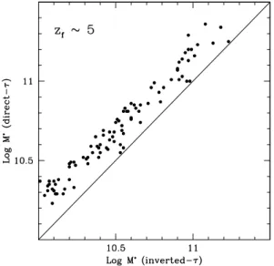
Figure 13.A comparison of the stellar masses derived assuming exponentially decreasing star formation rates (direct-τ models) with those obtained assuming exponentially increasing star for-mation rates (inverted-τ models). The beginning of star forfor-mation is set at the cosmic epoch corresponding to z = 5 for all models.
exponentially decreasing SFRs have been assumed also for galaxies at very high redshifts (e.g., z = 4 − 6; Stark et al. 2009).
For both the exponentially declining and increasing τ models, we identify the best-fitting SFHs, first allowing only values of τ > 0.3 Gyr. The results are shown in Figures 13-16, in which the parameters of the best-fitting models for these two SFHs are compared.
Figure 14.The same as in Figure 13, but for a comparison of the derived star formation rates.
Figure 13 compares the stellar masses obtained with the two SFHs, showing that those obtained with direct-τ models are systematically larger by ∼ 0.2 dex with respect to stellar masses derived using the inverted-τ models. Figure 14 shows the comparison of the SFRs, with the SFR from inverted-τ models being systematically higher by ∼ 0.5 dex, and there-fore the specific SFR turns out to be systematically higher by ∼ 0.7 dex. Figure 15 shows how different the τ values derived using the two SFHs are. Direct-τ models prefer very large τ ’s, up to ∼ 10 Gyr, which is to say that they prefer nearly constant SFRs. On the contrary, inverted-τ models
Figure 15.The same as in Figure 13, but for a comparison of the derived τ values.
Figure 16.The same as in Figure 13, but for a comparison of the derived values of the reddening E(B − V ) .
prefer short τ ’s, typically shorter than ∼ 0.5 Gyr, hence a SFR that is rapidly increasing with time.
Figure 15 gives the key to understand the physical ori-gin of the mass and SFR offsets between the two families of models. Being forced to put more mass at early times, direct-τ models pick very large τ ’s trying to find the best compromise for mass and SFR, and, compared to inverted-τ models, they overproduce mass at early times and not enough star formation at late times. On the other hand, these latter models by construction put very little mass at early times, and most of it is formed at late times. In order to compromise mass and SFR, they may overestimate the current SFR, and may be forced to hide part of it demanding more extinction.
Indeed, Figure 16 compares the reddening obtained with the two opposite SFH assumptions, showing that to obtain a good fit in the rest-frame UV the higher ongoing
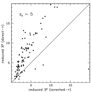
Figure 17.The same as in Figure 13, but for a comparison of the reduced χ2values of the best fit solutions.
SFR derived from inverted-τ models needs to be more dust-obscured than in the case of direct-τ models. Finally,
Fig-ure 17 compares the reduced χ2’s obtained with the two sets
of models. Those relative to inverted-τ models are not very good, but those with direct-τ models are definitely much worse. Still, a robust choice for the SFH cannot rely only on this relatively marginal advantage of inverted-τ models. In the next subsections we try to gather independent evidence that may help favouring one or the other option.
4.3 Comparing SFRs and extinctions from SED
fitting and from rest-frame UV only
The rest-frame UV part of the explored spectrum (from ob-served B band up to Spitzer/IRAC channel 3, i.e., 5.8 µm) is the one which most directly depends on the rate of on-going star formation. On the other hand, when the SFR is estimated with an SED-fitting procedure as in the previ-ous sections, the derived SFR results from the best-possible compromise with all the free parameters, given the adopted templates. In other words, the resulting SFR is
compro-mised relative to the other free parameters of the fit and
the adopted SFHs. SFRs from the UV flux, corrected for extinction using the UV slope (plus a reddening law, such as the Calzetti law, Calzetti et al. 2000) are widely derived in the literature for high redshift galaxies, and shown to be in very good agreement with independent estimates from the radio flux at 1.4 GHz (e.g., Reddy et al. 2004; Daddi et al. 2007a,b; Pannella et al. 2009), and also from the mid-IR (24 µm) and soft X-ray fluxes, for those galaxies with no mid-IR excess (Daddi et al. 2007b). Thus, the SFR derived only from the UV flux represents an uncompromised template (in the sense that it has no covariance with other parameters of the fit), and therefore with respect to which we may gauge the physical plausibility of a whole optical-near-IR SED fit. Figure 18 compares the E(B−V ) vs. SFR relations that are obtained from SED fittings with various SFHs, to those obtained using only the U V part of the spectrum. The latter ones were derived by Daddi et al. (2004, 2007a) using the
Bruzual & Charlot (2003) models for converting LUV into
SFR, following Madau et al (1998). E(B − V ) is derived by mapping the (B −z) colour into E(B −V ) using the Calzetti et al. law. Note that there are no appreciable differences in the UV between the models of Bruzual & Charlot (2003) and those of Maraston (2005) that are used in this paper. As clearly shown, the best agreement is between UV-derived SFRs and those obtained from SED fitting with inverted-τ models and fixed formation redshift. Notice that when leav-ing age as a free parameter several galaxies are found with exceedingly large SFRs and E(B − V ) values (see also Sec-tion 4.1), much at variance with the more robust values de-rived from the UV flux. Direct-τ models with fixed formation redshift are in better agreement with the UV-derived SFRs, yet they systematically underestimate the SFR as already noticed in Section 4.2.
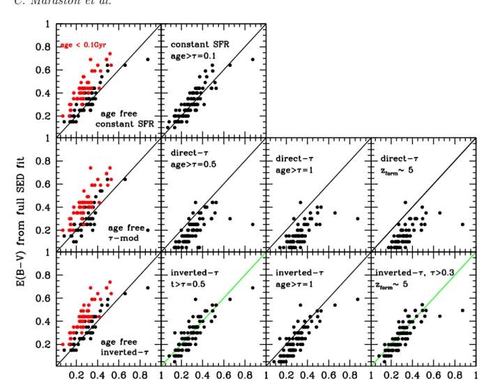
This is further illustrated in Figure 19 and Figure 20 which show the SFR and the reddening E(B − V ) from the SED fits directly compared to those from the UV. Among all explored SFHs, the inverted-τ models clearly are in best agreement with the values derived from the UV flux and slope. We interpret this as an indication that the SFHs of inverted-τ models models are closer to those of real galaxies, compared to the SFHs of direct-τ models.
4.4 Best fit solutions with fixed τ and age > τ
It is easy to realise that in galaxies that follow a SFR such as that given by Equation (1) the SFR tends to increase exponentially with time (Pannella et al. 2009; Renzini 2009). More precisely, if one ignores the t term in this equation the exponential increase proceeds with a τ ≃ 0.7 Gyr. Thus, in this Section we present the results of performing a new set of best fits, this time assuming a fixed τ (namely τ =0.5 and 1 Gyr, that bracket the empirical value), leaving age as a free parameter but constraining it to be larger than τ . We also consider the case of direct-τ models with the same parameters and restrictions. This choice to set limits on age may appear rather artificial, and indeed it is purely meant to avoid the extremely small ages that are found when age is left completely free. In practice, this exercise consists in considering only the cases with age > τ among those already explored in Section 4.1.
The comparison of the SFRs derived from direct- and inverted-τ models (Figure 21) is qualitatively similar to the case of fixed formation redshift (cf. Figure 14), and the same comments apply also here. The SFR and E(B − V ) values that are obtained with these further models are then com-pared to those obtained from the UV in Figures 19 and 20. It is apparent that inverted-τ models with τ =0.5 Gyr and ages larger than τ give results nearly as good as those de-rived for the case of fixed formation redshift. Also the case of SFR = constant and age > 0.1 Gyr SFRs results in reason-able agreement with those derived from the UV. All other explored SFHs give results at variance from those obtained from the UV, that we regard as the most robust method to estimate the SFR and reddening.
Figure 22 shows the derived stellar masses. In this pa-rameterisation there is less difference between the masses that are derived with the age > τ constraint with respect to the case of fixing the formation redshift. This is due to the fact that direct-τ models indicate lower masses compared
to those in the case of fixed formation redshift, because of their lower age, hence shorter duration of the star formation
activity. Note, however, that in most cases the smallest χ2r
are obtained for the smallest possible age, i.e., age≃ τ , or
∼0.5 Gyr, as shown in Figure 23, again a consequence of
the outshining effect.
4.5 Blind diagnostics of the star formation history
of mock galaxies
The ability of an adopted shape of the SFH to recover the ba-sic properties of a composite stellar population can be tested on mock galaxies with known SFHs. In a parallel project (J. Pforr et al., in preparation) we use synthetic galaxies from semi-analytic models (GALICS, Hatton et al. 2003) in which the input SSPs are the Maraston (2005) models in the rendi-tion of Tonini et al. (2009, 2010). Their observed-frame mag-nitudes at the various redshifts are then calculated, fed into Hyper-Z just as if they were relative to real observed galax-ies, and best fits are sought using various template composite
stellar populations.3Here we focus on an experiment
involv-ing the templates used in this paper, namely inverted- and direct-τ models and constant SF models, applied to mock star-forming galaxies at redshift 2. The model spectra are reddened according to the ongoing SFR, using the empiri-cal evidence that the E(B − V ) is proportional to the SFR (e.g., Daddi et al. 2007a) of each individual galaxy, with E(B − V ) = 0.33 × (log SFR − 2) + 1/3. Extinction as a function of wavelength is then applied following the law of Calzetti et al. (2000). Note that we do not take such mock galaxies as representative of real galaxies. The goal of the experiment is to show what happens if the SED of a galaxy with a certain SFH is used to derive its SFR and stellar mass using a different SFH.
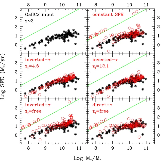
Figures 24 and 25 show the results. The upper left panel of Figure 24 shows the input values, i.e. the distribution of SFRs and masses of the semi-analytic models at redshift 2 (black points). The other panels show the output values, i.e. the SFRs and masses that are obtained by fitting the SED of the mock galaxies with the various templates, as indicated, over-plotted to the input values.
The inverted-τ models with fixed formation redshift can recover the input quantities strikingly well (middle panels).
Towards the low-mass end (M∼< 109M⊙) the SFR is
some-what underestimated, suggesting that the assumed start of SF is too early. Note also, as shown by the two middle pan-els in Figure 24, that the result is almost independent of the assumed formation redshift, as already argued in Section 4.2.
None of the other SFH templates do as well. With the free age mode a substantial number of outliers with very high SFRs are obtained. The green line in Figure 24 and Figure 25 is a fit to the outliers found among the real GOODS galaxies from the direct-τ models (the blue objects in Figure 19 and Figure 20), and it is quite instructive to note that when the
3 A similar project is described in Wuyts et al. (2009a), and a
detailed comparison with their results is given in Pforr et al., in preparation. The systematic offsets introduced by the use of direct-τ models to derive masses and SFRs of mock galaxies at z >3 are also investigated by Lee et al. 2009).
Figure 18.The reddening and SFRs derived under different assumptions on the SFH are compared to those derived using only the rest-frame UV part of the spectrum (red points), i.e., the wavelength range that most directly depends on the ongoing rate of star formation. The upper panel shows a comparison of such UV-derived SFRs with those derived from SED fitting assuming SFR=const and leaving age as a free parameter. In the middle panel the comparison is made with inverted-τ models, with both fixed and free age (black and grey points, respectively). Finally, the lower panel shows the comparison with the direct-τ -models.
fit produces wrong values, those follow the same relation of fake values in mock galaxies. Finally, Figure 25, analogous to Figure 24, shows the result of the same experiment with mock galaxies, but now using the template SFHs discussed in the previous subsection, i.e., with fixed τ and age > τ . The inverted-τ models with age > τ , and τ = 0.5 Gyr give fairly good fits to the actual values in the mock galaxies, but not as good as those with a prior on the formation red-shift (see Figure 24, middle panels). Finally, note that some outliers among the mock galaxies, a few with low SFR for their masses (hence almost passive), are poorly reproduced by the explored SFHs, as all assume that star formation is still going on.
The reason why inverted-τ models fit better is very simple. Most mock galaxies constructed from semi-analytic models exhibit secularly increasing SFRs, as do the cold-stream hydrodynamical models of Dekel et al. (2009) as one expects from the empirical SFR-mass relation (e.g., Ren-zini 2009). Therefore, we believe that quite enough argu-ments militate in favour of preferring exponentially increas-ing SFRs, as opposed to decreasincreas-ing or constant.
4.6 Allowing very small values ofτ
As one can notice from Figure 15, using inverted-τ models the vast majority of the best fits tend to cluster close to the minimum allowed value of τ , i.e., 0.3 Gyr, a limit that was imposed based on the value of τ implied by the empirical
SFR−M∗ relation, as discussed in Section 4.4. But what
happens if this limit is removed, and the best fit procedure is allowed to chose any value of τ down to 0.05 Gyr? The results are shown in Figure 26: several galaxies are now “best fitted” with very small τ ’s, implying SFHs in which most
Figure 21.Comparison of the star formation rates derived as-suming exponentially decreasing star formation rates (direct-τ models) with those obtained assuming exponentially increasing star formation rates (inverted-τ models). In both models, τ has been fixed to two values of 0.5 and 1 Gyr, and the age is con-strained to be larger than τ .
stars formed just shortly before the time at which the galaxy is observed. This is to say that leaving the procedure free to choose very small values of τ results in best fits that closely resemble those obtained with age as a free parameter, that were discussed (and rejected) in Section 4.1. Figure 26 shows that also in this case SFRs well in excess of those derived from the UV are derived for several galaxies. Therefore, also inverted-τ models with unconstrained τ ’s suffer from the outshining phenomenon that plagues models with age as a fully unconstrained free parameter.
Figure 19.The comparison of SFRs derived from SED fitting with those derived from the rest-frame UV only (plus extinction correction). Inverted-τ models with zform= 5 (or inverted-τ s with fixed τ =0.5 Gyr and ages constrained to be larger than τ ) provide the best result
(panels with green lines).
10.5 11
10.5 11
Figure 22.The same as in Figure 21, but for a comparison of the derived stellar masses.
The lesson we learn from these experiments is that only by setting a prior on age one derives astrophysically more acceptable solutions. Depending on the adopted shape of the
Figure 23.Distributions of the ages obtained with models with fixed τ and ages constrained to be larger than τ , for τ = 0.5 Gyr (black histogram) and τ − 1 Gyr (shaded histogram).
SFH, this prior can be a minimum age (for constant SFR models), or setting age> τ (for direct-τ models), or finally
Figure 20.The same as Figure 19 for the reddening E(B − V ). Conclusions are identical.
setting a minimum acceptable value for τ (for inverted-τ models). This kind of fix looks quite artificial, and admit-tedly the resulting procedure is far from being elegant. It is a simple way of avoiding the outshining effect, and obtain SFRs that are in agreement with those derived from other direct methods, such as from UV, radio, or mid-IR (e.g., Daddi et al. 2007a,b; Pannella et al 2009).
4.7 How robust are stellar mass estimates?
While SFR and reddening can be best evaluated by just us-ing the UV part of a galaxy’s spectrum, the determination of the stellar mass, such a crucial quantity for understanding galaxy evolution, requires the full SED fitting. Hence, it re-quires exploring a variety of assumed SFHs. We have shown that there are some adopted SFHs that, constrained to avoid the outshining problem, give SFRs and E(B − V ) values in excellent agreement with those derived from the UV. Now, how different are the derived stellar masses when using these viable options for the SFH? And, ultimately, how much can we trust such derived masses?
Figure 27 - first and second panel - compares the stellar masses that are derived for the real galaxies studied in this paper using these viable SFHs, namely inverted-τ with high
formation redshift, inverted-τ with age constrained, and con-stant SF with age constrained. The corrensponding masses agree with each other quite well, systematic differences are
quite small (∼< 0.1 − 0.2 dex), and also the scatter is quite
modest, of the order of 0.1 dex. Can this consistency suffice to conclude that the adopted procedures give a robust esti-mate of stellar masses? In this respect, the fairly accurate recovery of the masses of mock galaxies should increase our confidence.
Yet, the problem of outshining remains. What we con-sider viable options are SFHs described by extremely sim-ple functions, i.e., either constant or exponential. Nature certainly realises far more complex SFHs. For example, an early burst of star formation, followed by a continuous SFR, could be easily missed by the best fit procedure, by remain-ing out-shined by the successive and ongoremain-ing star formation. Thus, we suspect that derived masses may underestimate the actual stellar mass, at least for those galaxies with early massive starbursts.
We note that Figure 27, third panel compares also the masses derived from direct-τ models with unconstrained age, to those derived from the viable SFHs. Clearly, such direct-τ models can substantially underestimate the stellar mass, while they overestimate the SFR (cf. Figure 19).
To conclude this section, Figure 28 shows the absolute values of the stellar mass of star-forming galaxies at redshift z ∼ 2 that are obtained using our preferred star formation history.
5 DISCUSSION AND CONCLUSIONS
We have tried different priors for the SFH of z ∼ 2 galaxies,
and used a χ2 best fit approach to derive the basic
prop-erties of such galaxies: SFR, stellar mass, reddening, age, etc. We do not expect that any of the simple mathematical forms adopted for the SFH (constant SFR, exponentially de-creasing, exponentially increasing) is strictly followed by real galaxies. We expect, however, that the two opposite choices for the exponential case are sufficiently extreme to encom-pass the real behavior of galaxies, or at least those having experienced a quasi-steady SFR over most of their lifetime. We try various tests to distinguish which of the various op-tions is the most acceptable one (or the least unacceptable) for giving the astrophysically most plausible values for the basic properties of star forming galaxies in the redshift range between ∼ 1.4 and ∼ 2.5.
We find that by leaving age as a free parameter the best fit procedure delivers implausibly short ages, no mat-ter which SFH template is adopted. This is so because the SED is dominated by the stars that have formed most re-cently, and they outshine the older stellar populations that may inhabit these galaxies. Thus, introducing a prior on the beginning of star formation appears to be necessary.
Assuming that star formation started at high redshift (i.e., z >>∼ 2, the precise value being almost irrelevant) provides a more credible framework, with models with ex-ponentially increasing SFR (that we call inverted-τ models) giving systematically higher SFRs for the z ∼ 2 galaxies in the test sample, and lower stellar masses, compared to mod-els with exponentially decreasing SFR. These two systematic differences together imply a specific SFR that is a factor of
∼5 higher in inverted-τ models, compared to direct-τ
mod-els, when star formation is assumed to start at high redshift (e.g., z = 5) in both cases.
On the other hand, inverted-τ models offer various no-table advantages: 1) they indicate SFRs and extinctions in excellent agreement with those derived from the rest-frame UV part of the SED, which most directly relates to the on-going star formation and reddening, 2) they fairly accurately recover the SFRs and masses of mock galaxies constructed from semi-analytic models, in which SFR are indeed secu-larly increasing in most cases, and 3) have systematically
better reduced χ2 values compared to models with
expo-nentially decreasing SFRs, though one cannot consider them fully satisfactory. These advantages are somewhat reduced if the best fit procedure is allowed to pick very small values of τ , down to 0.05 Gyr, as in such case derived SFRs tend to be somewhat overestimated compared to those derived from the UV.
We have also explored star formation histories (such as constant SFR, or exponentially decreasing) in which age is a priori constrained to avoid very small values (e.g., age > 0.1 Gyr, or age > τ , or fixed τ ). Adopting such priors, though it may seem quite artificial, gives more plausible solutions with respect to cases in which age is left fully free. This is due to
the mentioned outshining effect of very young stellar popu-lations over the older ones. Still, models with exponentially increasing SFRs tend to give systematically better results, as judged from the consistency with the UV derived SFRs. Besides the above arguments, there are other reasons to prefer stellar population models constructed with exponen-tially increasing SFRs, including:
1) The almost linear relation between SFR and stellar mass
(SFR ∝ ∼ M∗), and the small scatter about it, that are
empirically established for redshift ∼ 2 galaxies implies that they can indeed experience a quasi-exponential growth at these cosmic epochs. Later, some process may quench their star formation entirely and turn them into passively evolving ellipticals, or keep growing until the secular decrease of the
specific star formation rate (the t−2.5 term in Equation (1))
takes over, and galaxies (such as spirals) continue forming stars at a slowly decreasing rate all the way to the present epoch (Renzini 2009).
2) The direct observation of the evolution of the luminosity function in rest-frame UV (which is directly related to SFR)
shows that the characteristic luminosity at 1600 ˚A (M∗
1600)
brightens by over one magnitude between z = 6 and z = 3 (Bouwens et al. 2007). Since extinction is likely to increase with time following metal enrichment, the increase of the rest-frame UV luminosity can only be due to an increased SFR in individual galaxies.
The aim of this paper is to explore which assumptions and procedures are likely to give the most robust estimates of the basic stellar population parameters, when using data that extend from the rest-frame UV to the neIR. We ar-gue that ongoing SFRs are best derived at wavelengths be-low about one micron by using the UV part of the SED of galaxies, and inverted-τ models give SFRs in excellent agreement with them. However, the fit to the full optical to near-infrared SED is required to derive the mass in stars. We show that the SFHs, with a prior on age or τ to re-duce the outshining effect, give results that agree quite well with each other, giving some confidence on the reliability of the derived masses. However, it is still possible that the mass may be somewhat underestimated for those galaxies in which a substantial fraction of the stellar mass was produced in a strong burst, early in their evolution.
At first sight the higher SFRs and lower stellar masses indicated by inverted-τ models (compared to direct-τ mod-els, both with fixed formation redshift) may exacerbate an apparent mismatch between the cosmic (volume averaged)
SFR history ( ˙ρ∗(z)) and the empirical stellar mass
den-sity (ρ∗(z)), such that the integration of SFR(z) tends to
overproduce the stellar mass density at most/all redshifts (e.g., Wilkins, Trentham & Hopkins 2008). However, SFRs are more often derived from direct SFR indicators, such as the rest-frame UV, radio flux, Hα flux, or mid/far-infrared, rather than from SED fits. Therefore the 0.5 dex effect on the SFRs relative to the direct-τ models should not affect this discrepancy. There may remain the 0.2 dex effect on the masses, but inverted-τ models, by construction minimising star formation at early times, may systematically under-estimate the stellar mass of galaxies, in particular if part of it was formed in early bursts. Thus, with this caveat in mind, the use of inverted-τ models with fixed formation red-shift should not appreciably exacerbate the mismatch prob-lem mentioned above. Instead, direct-τ models with
uncon-Figure 24.Comparison between the input values of SFR and stellar mass of Mock galaxies from semi-analytic models (labelled as GALICS, black points) and the same quantities derived from SED fitting using the various templates (labelled in each panel, red points). The green line highlights the position of the fake outliers.
strained age most certainly worsen this problem as they un-derestimate the stellar mass (see Figure 27, right panel), and overestimate the SFR (see Figure 19).
We conclude that the use of synthetic stellar popula-tions with an exponentially declining SFR should be avoided in the case of star forming galaxies at redshift beyond
∼ 1. Exponentially increasing SFRs, with e-folding times
of ∼ 0.3 − 1 Gyr, and a high starting redshift appear to provide astrophysically more plausible results, and while na-ture may not closely follow such a simple functional behav-ior, they should be preferred in deriving SFRs and stellar masses of high redshift galaxies. In any event, we believe that maximum likelihood parameters are not necessarily unbiased estimators of star formation rates and masses of
high-redshift galaxies, but the broadest possible astrophys-ical context should be considered.
ACKNOWLEDGMENTS
We thank the referee Stephen Serjeant for a prompt and useful report. We are grateful to Andi Burkert for valu-able comments on a very early draft of the paper, and to Laura Greggio and Daniel Thomas for useful discus-sions. We acknowledge Micol Bolzonella for her construc-tive help with the Hyper-Z code. CM, JP, and CT acknowl-edge the Marie-Curie Excellence Team grant ”Unimass”, ref. MEXT-CT-2006-042754 of the Training and Mobility of Re-searchers programme financed by the European Community.
Figure 25.The same as Figure 24, for the cases in which τ has been fixed to the indicated values, with the additional restriction imposing the age to exceed τ .
1 2 3 1 2 3 0 0.2 0.4 0.6 0.8 1 0.2 0.4
Figure 26. Left panel: The SFR from the full optical-to-near-IR SED fit derived from inverted-τ models in which τ is allowed to take very small values, compared to the SFR derived only from the UV part of the SED. Right panel: The frequency histogram of the corresponding values of τ .
ED acknowledges the funding support of the ERC-StG grant UPGAL-240039, ANR-07-BLAN-0228 and ANR-08-JCJC-0008. AR is grateful for the hospitality of the ICG during the final rush for the completion of this paper. Some of the data used here are part of the GOODS Spitzer Space Tele-scope Legacy Science Program, that is supported by NASA
through Contract Number 1224666 issued by the JPL, Cal-tech, under NASA contract 1407.
REFERENCES
Figure 27.A comparison of the stellar masses derived for the GOODS galaxies from inverted-τ models, with zf = 5 and τ > 0.3 Gyr, with those derived from other adopted SFHs. Left panel: vs. inverted-τ models with age > τ = 0.5 Gyr; Central panel: vs. models with SFR=const. and age> 0.1 Gyr; Right panel: vs. direct-τ models and unconstrained age.
Figure 28.Stellar masses for the z ∼ 2 GOODS star-forming galaxies as derived from inverted-τ models, with zf ∼> 5 and τ > 0.3 Gyr.
Bouwens R. J., Illingworth G. D., Franx M., Ford H., 2007, ApJ, 670, 928
Brinchmann J., Charlot S., White S. D. M., Tremonti C., Kauff-mann G., Heckman T., BrinkKauff-mann J., 2004, MNRAS, 351, 1151
Bruzual A. G., 1983, ApJ, 273, 105
Bruzual G., Charlot S., 2003, MNRAS, 344, 1000
Calzetti D., Armus L., Bohlin R. C., Kinney A. L., Koornneef J., Storchi-Bergmann T., 2000, ApJ, 533, 682
Chabrier G., 2003, PASP, 115, 763
Cimatti A., Cassata P., Pozzetti L. et al., 2008, A&A, 482, 21
Daddi E., Cimatti A., Renzini A., Fontana A., Mignoli M., Pozzetti L., Tozzi P., Zamorani G., 2004, ApJ, 617, 746 Daddi E., Dickinson M., Chary R. et al., 2005, ApJ, 631, L13 Daddi E., Renzini A., Pirzkal N. et al., 2005, ApJ, 626, 680 Daddi E., Dickinson M., Morrison G. et al., 2007, ApJ, 670, 156 Daddi E., Alexander D. M., Dickinson M. et al., 2007, ApJ, 670,
173
Daddi E., Dannerbauer H., Stern D. et al., 2009, ApJ, 694, 1517 Dekel A., Birnboim Y., Engel G. et al., 2009, Nat, 457, 451 Elbaz D., Daddi E., Le Borgne D. et al., 2007, A&A, 468, 33 Fontana A., Santini P., Grazian A. et al., 2009, A&A, 501, 15 F¨orster Schreiber N. M., Genzel R., Bouch´e N. et al., 2009, ApJ,
706, 1364
Genzel R., Tacconi L. J., Eisenhauer F. et al., 2006, Nat, 442, 786 Giavalisco M., Ferguson H. C., Koekemoer A. M. et al., 2004,
ApJ, 600, L93
Gonzalez V., Labbe I., Bouwens R. J., Illingworth G. Franx M., Kriek M., Brammer G. B., 2010, ApJ, 713, 115
Hatton S., Devriendt J. E. G., Ninin S., Bouchet F. R., Guider-doni B., Vibert D., 2003, MNRAS, 343, 75
Hopkins A. M., Beacom J. F., 2006, ApJ, 651, 142
Kennicutt R.C., 1986, in Norman C. A., Renzini A., Tosi M., eds, Stellar Populations. Cambridge Univ. Press, p. 125
Kong X., Daddi E., Arimoto N. et al., 2006, ApJ, 638, 72 Kroupa P., 2001, MNRAS, 322, 231
Kurk, J., Cimatti A., Daddi E. et al., 2009, The Messenger, 135, 40
Lee S.-K., Idzi R., Ferguson H. C., Somerville R. S., Wiklind T., Giavalisco M., 2009, ApJS, 184, 100
Madau P., Pozzetti L., Dickinson M., 1998, ApJ, 498, 106 Maraston C., 1998, MNRAS, 300, 872
Maraston C., 2005, MNRAS, 362, 799
Maraston C., Daddi E., Renzini A., Cimatti A., Dickinson M., Papovich C., Pasquali A., Pirzkal N., 2006, ApJ, 652, 85 Men´endez-Delmestre K., Blain A. W., Smail I. et al., 2009, ApJ,
699, 667
Noeske K. G., Weiner B. J., Faber S. M. et al., 2007, ApJ, 660, L43
Noll S., Pierini D., Cimatti A. et al., 2009, A&A, 499, 69 Pannella M., Carilli C. L., Daddi E. et al., 2009, ApJ, 698, L116 Papovich C., Dickinson M., Ferguson H. C., 2001, ApJ, 559, 620 Popesso P., Dickinson M., Nonino M. et al., 2009, A&A, 494, 443
Pozzetti L., Bolzonella M., Zucca E. et al., 2009, preprint (arXiv:0907.5416)
Reddy N. A., Steidel C. C., 2004, ApJ, 603, L13 Renzini A., 2009, MNRAS, 398, L58
Retzlaff J., Rosati P., Dickinson M., Vandame B., Rite C., Nonino M., Cesarsky C., the GOODS Team, 2010, A&A, in press Schinnerer E., Smolˇci´c V., Carilli C. L. et al., 2007, ApJS, 172,
46
Shapley A. E., Steidel C. C., Erb D. K., Reddy N. A., Adelberger K. L., Pettini M., Barmby P., Huang J. 2005, ApJ, 626, 698 Serjeant S., Gruppioni C., Oliver S., 2002, MNRAS, 330, 621 Stark D. P., Ellis R. S., Bunker A., Bundy K., Targett T., Benson
A., Lacy M., 2009, ApJ, 697, 1493
Tacconi L. J., Genzel R., Smail I. et al., 2008, ApJ, 680, 246 Tonini C., Maraston C., Devriendt J., Thomas D., Silk J., 2009,
MNRAS, 396, L36
Tonini C., Maraston C., Thomas D., Devriendt J., Silk J., 2010, MNRAS, 403, 1749
Vanzella E., Cristiani S., Dickinson M. et al., 2008, A&A, 478, 83 Wilkins S. M., Trentham N., Hopkins A. M., 2008, MNRAS, 385,
687
Williams R. J., Quadri R. F., Franx M., van Dokkum P., Labb´e I., 2009, ApJ, 691, 1879
Wuyts S., Franx M., Cox T. J., Hernquist L., Hopkins P. F., Robertson B. E., van Dokkum P. G., 2009, ApJ, 696, 348 Wuyts S., Franx M., Cox T. J. et al., 2009, ApJ, 700, 799