Intermittent chaos driven by nonlinear Alfvén waves

(1)

HAL Id: hal-00302411

https://hal.archives-ouvertes.fr/hal-00302411

Submitted on 16 Dec 2004

HAL is a multi-disciplinary open access

archive for the deposit and dissemination of

sci-entific research documents, whether they are

pub-lished or not. The documents may come from

teaching and research institutions in France or

abroad, or from public or private research centers.

L’archive ouverte pluridisciplinaire HAL, est

destinée au dépôt et à la diffusion de documents

scientifiques de niveau recherche, publiés ou non,

émanant des établissements d’enseignement et de

recherche français ou étrangers, des laboratoires

publics ou privés.

Intermittent chaos driven by nonlinear Alfvén waves

E. L. Rempel, A. C.-L. Chian, A. J. Preto, S. Stephany

To cite this version:

E. L. Rempel, A. C.-L. Chian, A. J. Preto, S. Stephany. Intermittent chaos driven by nonlinear

Alfvén waves. Nonlinear Processes in Geophysics, European Geosciences Union (EGU), 2004, 11

(5/6), pp.691-700. �hal-00302411�

(2)

Nonlinear Processes in Geophysics (2004) 11: 691–700

SRef-ID: 1607-7946/npg/2004-11-691

Nonlinear Processes

in Geophysics

Intermittent chaos driven by nonlinear Alfv´en waves

E. L. Rempel, A. C.-L. Chian, A. J. Preto, and S. Stephany

National Institute for Space Research (INPE) and World Institute for Space Environment Research (WISER), P.O. Box 515, S˜ao Jos´e dos Campos–SP, 12227–010, Brazil

Received: 14 September 2004 – Revised: 9 December 2004 – Accepted: 14 December 2004 – Published: 16 December 2004 Part of Special Issue “Advances in space environment turbulence”

Abstract. We investigate the relevance of chaotic saddles and unstable periodic orbits at the onset of intermittent chaos in the phase dynamics of nonlinear Alfv´en waves by us-ing the Kuramoto-Sivashinsky (KS) equation as a model for phase dynamics. We focus on the role of nonattracting chaotic solutions of the KS equation, known as chaotic sad-dles, in the transition from weak chaos to strong chaos via an interior crisis and show how two of these unstable chaotic saddles can interact to produce the plasma intermittency ob-served in the strongly chaotic regimes. The dynamical sys-tems approach discussed in this work can lead to a better un-derstanding of the mechanisms responsible for the phenom-ena of intermittency in space plasmas.

1 Introduction

Intermittent fluctuations are constantly encountered in space plasmas, as reported in several works based on the analysis of solar wind data both at the ecliptic (Burlaga, 1991; Marsch and Tu, 1993; Bruno et al., 2003) and high heliographic lat-itude (Ruzmaikin et al., 1995; Pagel and Balogh, 2003). In-termittent events are characterized by time series that dis-play time intervals with low variabilities interrupted by bursts of very high variabilities. As a consequence, the associated probability density functions (PDF’s) are non-Gaussian. It has been shown by Vörös et al. (2002) and Dorotovic and Vörös (2004) that intermittent fluctuations in the solar wind affect the geomagnetic response. By comparing solar wind data obtained from the ACE spacecraft with plasma sheet data from the Geotail mission, Dorotovic and Vörös (2004) suggested that the non-Gaussian characteristics of the PDF’s of solar wind data can be interconnected to the occurrence of intermittency in the magnetic fluctuations in the plasma sheet. Thus, the study of intermittent phenomena in solar

Correspondence to: E. L. Rempel

([email protected])

wind plasmas is essential for a better understanding of the solar wind-magnetosphere coupling processes.

The fluctuations of the plasma velocity and magnetic field as revealed by interplanetary data records are frequently well correlated, which is a signature of the presence of Alfvén waves in the solar wind (Belcher and Davis, 1971; Goldstein and Roberts, 1995). Alfvén waves are low-frequency elec-tromagnetic waves in a plasma with a background magnetic field. From a linear analysis of MHD equations, the disper-sion relation of the Alfvén wave is found as ω=k||vA, where k||is the component of the wave vector k parallel to B0, and

vA=B0/(µ0ρ0)1/2 is the Alfv´en velocity, where B0 is the

strength of the ambient magnetic field, µ0is the permeability

of vacuum and ρ0is the average mass density of the plasma.

The perturbation of the fluid velocity u relates to the mag-netic field’s perturbation vector b=δB0by u=∓b/(µ0ρ0)1/2,

where the upper (lower) sign refers to the case k · B0>0

(k · B0<0). Thus, u and b are parallel/antiparallel and

pro-portional to each other, and the plasma oscillates with the magnetic field lines.

As shown by Lefebvre and Hada (2000), by assuming weak instability the dynamics of quasiparallel Alfv´en waves can be studied by a complex Ginzburg-Landau (CGL) equa-tion. The complex Ginzburg-Landau equation has been one of the most widely studied nonlinear equations in the last decades (see Cross and Hohenberg, 1993; Bohr et al., 1998; Aranson and Kramer, 2002, and references therein). It de-scribes the slow modulation of a periodic pattern in space and time near the threshold of an instability, where a band of modes become unstable.

In this work we study the phase dynamics of nonlinear Alfv´en waves modeled by the CGL equation. Phase dynam-ics is of particular interest in systems modeled by the CGL equation, since for a range of values of the control parameters the dynamics of perturbations of traveling wave solutions is essentially determined by variations of the phase alone, and can exhibit “phase turbulence”. In such regimes the ampli-tudes are essentially constant and the phase dynamics sat-isfies the Kuramoto-Sivashinsky (KS) equation (Kuramoto

(3)

692 E. L. Rempel et al.: Intermittent chaos driven by nonlinear Alfv´en waves and Tsuzuki, 1976; Cross and Hohenberg, 1993; Bohr et al.,

1998; Aranson and Kramer, 2002; van Baalen, 2004). The study of phase dynamics can elucidate important nonlinear phenomena observed in space plasmas. Finite correlation of phases in MHD waves upstream of Earth’s bow shock was found in Geotail magnetic field data, indicating that non-linear interactions between the waves are in progress (Hada et al., 2003). This bears important implications in discus-sions of various transport processes of charged particles in space. In He and Chian (2003) imperfect phase synchro-nization in a nonlinear drift wave system was shown to be responsible for the origin of bursts in wave energy in a tur-bulent state. Here we focus on the characterization of phase intermittency in the KS equation. We first describe how the fluctuations of the phase can evolve from periodic to chaotic behavior through a sequence of bifurcations as the viscosity is varied. We show that in the KS equation, chaotic attractors coexist with nonattracting chaotic sets responsible for tran-sient chaotic behavior. The collision of a weak chaotic at-tractor with an unstable periodic orbit leads to the generation of a strong chaotic attractor, in an event known as interior crisis. The post-crisis strong chaotic attractor can be decom-posed into two nonattracting chaotic sets, responsible for the generation of intermittent time series.

Section 2 of this paper contains a brief introduction to ba-sic concepts on nonlinear dynamical systems. In Sect. 3 we describe the numerical solutions of the KS equation by the Galerkin spectral method. In Sect. 4 we present our analysis of attracting and nonattracting chaotic sets in the KS equa-tion. The conclusions are given in Sect. 5.

2 Basic concepts of nonlinear dynamics

In this section we review some basic concepts of nonlinear dynamical systems (Parker and Chua, 1989; Ott, 1993; Al-ligood et al., 1996) that are essential for understanding the remaining of this paper.

We consider dissipative dynamical systems described by autonomous systems of ODE’s,

˙

x = f (x), (1)

where x is an n-dimensional vector, f is a vector function and the dot denotes derivative with respect to time. A “flow”

ft(x0)is the solution of Eq. (1) for an initial condition x0 after certain time t . The components of the vector “state variable” x define a “phase space”, where the flow of x0is

plotted for increasing values of t, generating the “orbit” of

x0.

A “fixed point” of Eq. (1) is a constant solution, i.e. a point

¯

x for which ˙x=0, or equivalently, ft( ¯x)= ¯x for all t. A

“pe-riodic orbit” is a solution of Eq. (1) that always repeats its behavior after a fixed time interval, i.e. ft(x)=ft +T(x) for

all t and some minimum period T >0.

Dissipative systems are characterized by the presence of “attractors”. An attractor is a subset of the phase space that

attracts almost all the initial conditions in a certain neighbor-hood, that is, the limit set of the orbits of initial conditions in the neighborhood as time tends to +∞ is the attractor (Gre-bogi et al., 1984). Attractors may be simple sets like a fixed point or periodic orbit, but can also have nonelementary ge-ometrical properties such as noninteger fractal dimension, in which case the attractor is called “strange” (Grebogi et al., 1984, 1987b). Fractal sets display scale invariance, which implies that continuous blow-up of a tiny portion of the set reveal self-similar structures on arbitrarily small scales (Ott, 1993).

Strange attractors are typically (but not always) “chaotic” (Grebogi et al., 1987b). The orbits of random initial con-ditions on a chaotic attractor will display aperiodic behav-ior and “sensitive dependence on initial conditions”, which means that nearby orbits will diverge exponentially with time. The average rate of divergence can be measured by the “Lyapunov exponent”. Let 10be a small distance separating

two initial conditions on the chaotic attractor at t=0. Then for increasing t the orbits of the two points will diverge on average as 1t∼10exp(λt ), where λ is the Lyapunov

expo-nent (Grebogi et al., 1987b). For systems with n-dimensional phase space there are n Lyapunov exponents which measure the rate of divergence/convergence on n orthogonal direc-tions.

Chaotic sets are not necessarily attracting sets. A strange set 3 might be chaotic and nonattracting. That means that the orbits of typical initial conditions in the vicinity of 3 are eventually repelled from it. Nevertheless, 3 contains a chaotic orbit (an aperiodic orbit with at least one positive Lyapunov exponent) (Nusse and Yorke, 1989). If the chaotic orbit has also one negative Lyapunov exponent the nonat-tracting chaotic set is known as “chaotic saddle”. Chaotic saddles, as well as chaotic attractors, contain an infinite num-ber of unstable periodic orbits (UPO’s).

In nonlinear dynamical systems, as one varies some con-trol parameter present in the model equations some dynam-ical changes can occur, such as creation/destruction of fixed points and periodic orbits or loss of stability of attracting sets. Thus, periodic attractors can lose their asymptotic stability and become unstable periodic orbits. Similarly, chaotic at-tractors can lose their attracting nature and become nonat-tracting chaotic sets, or chaotic saddles. The qualitative changes in the behavior of solutions of dynamical systems as a control parameter is varied are called “bifurcations”. When the changes in the phase portrait involve merely the local vicinity of fixed points or periodic orbits, one has a “lo-cal bifurcation”. Large changes in the topology of the system are called “global bifurcations”. An example is the “interior crisis” discussed in this paper, whereby a chaotic attractor is suddenly enlarged. The bifurcations of a dynamical system can be represented in a “bifurcation diagram”, in which the values of one of the state variables are plotted as a function of one control parameter.

A classical technique to analyze nonlinear dynamical systems is the “Poincar´e map”. It replaces the flow of an nth-order continuous-time system with an (n−1)th-order

(4)

E. L. Rempel et al.: Intermittent chaos driven by nonlinear Alfv´en waves 693 discrete-time system, simplifying the analysis and

visualiza-tion of the dynamics. There are different forms of defining a Poincar´e map. At the end of the next section we exemplify one of them.

3 The Kuramoto-Sivashinsky equation

The derivative nonlinear Schrödinger equation (DNLS) (Rogister, 1971; Mjolhus and Wyller, 1988) describes the dynamics of quasiparallel Alfvén waves of moder-ate amplitudes in a finite-β plasma, taking into account weak linear dispersion. To describe patterns formed by Alfvén waves subject to damping and growth rate, Lefebvre and Hada (2000) used a model based on a modified version of the DNLS equation, including lin-ear growth rate, linlin-ear dissipation and nonlinlin-ear Lan-dau damping. Assuming weak instability, Lefebvre and Hada (2000) proposed a further simplification to an en-velope equation by writing the complex transverse mag-netic field B=By+iBzas B(x, t )=ψ (ξ, t ) exp[i(kcx−ωct )],

where ωc=ω(kc), ξ =x−v(kc)t and kc is the most unstable

mode. Assuming kc>0 (left-hand polarization) the resulting

equation for ψ is given by

∂tψ = ψ + (1 − ib1)∂ξ ξψ − iψ (b2−H )|ψ |2, (2)

where b1measures the strength of the dispersion and b2the

effects of nonlinearity. The term H denotes a function that accounts for the nonlinear Landau damping (Mjolhus and Wyller, 1988). Equation (2) falls into the general class of the complex Ginzburg-Landau equation. The envelope ψ is a complex variable. By writing ψ =R exp(i8) and assum-ing small perturbations R=R0+r, 8=80+φ, it is possible

to derive an equation for the phase φ of the CGL equation. As shown by Kuramoto and Tsuzuki (1976) and Aranson and Kramer (2002), the phase equation is given by the Kuramoto-Sivashinsky equation. Here we study the following form of the KS equation (LaQuey et al., 1975; Christiansen et al., 1997; Chian et al., 2002; Rempel and Chian, 2003)

∂tφ = −∂x2φ − ν∂x4φ − ∂xφ2, (3)

where ν is a damping parameter representing viscosity and we assume that φ (x, t ) is subject to periodic boundary con-ditions

φ (x, t ) = φ (x +2π, t ). (4)

To obtain the numerical solution of Eq. (3) we use the Galerkin method (Gottlieb and Orszag, 1977), by applying a Fourier decomposition for the function φ(x, t )

φ (x, t ) = ∞ X k=−∞

bk(t )eikx. (5)

After substituting Eq. (5) into Eq. (3) and solving the derivatives one obtains

∞ X k=−∞ ˙ bkeikx= ∞ X k=−∞ k2bkeikx−ν ∞ X k=−∞ k4bkeikx − ∞ X k=−∞ ∞ X m=−∞ i(k + m)bkbmeix(k+m). (6)

Next, multiply Eq. (6) by e−ilx, with l=−∞, ..., ∞, and integrate in the spatial domain,

Z 2π 0 ∞ X k=−∞ ˙ bkeix(k−l)dx = Z 2π 0 ∞ X k=−∞ k2bkeix(k−l)dx − Z 2π 0 ν ∞ X k=−∞ k4bkeix(k−l)dx − Z 2π 0 ∞ X k=−∞ ∞ X m=−∞ i (k + m) ×bkbmeix(k+m−l)dx. (7)

Each integral of the exponential functions in Eq. (7) van-ishes except when the exponent is zero. The three first nents are zero when k=l. For the nonlinear term the expo-nent is null when k=l−m. After solving the integrals, Eq. (7) becomes ˙ bk =(k2−νk4)bk−ik N X m=−N bmbk−m, (8) k = −N, ..., N,

where N is the truncation order. Our choice of N is explained later in this section.

The coefficients bk in Eq. (8) are complex. We can

sim-plify our analysis by restricting to the subspace of odd solu-tions, φ (x, t )=−φ (−x, t ). It is possible to prove that if an initial condition φ (x, 0) is an odd function, the solution of Eq. (3) is odd for all time (Temam, 1988)

φ (x, t ) = −φ (−x, t ), ∀x, t. (9) The Fourier transform of an odd function has purely imag-inary coefficients, so we can represent odd functions by as-suming that bk(t )are purely imaginary, setting

bk = −

1

2iak, (10)

where ak are real numbers. After substituting Eq. (10) into

Eq. (8), we obtain ˙ ak =(k2−νk4)ak− k 2 N X m=−N amak−m, (11) k = −N, ..., N.

Equation (11) contains unnecessary operations. Since

φ (x, t )is real, −iak=ia−k, and it is not necessary to

com-pute the modes with negative k. Moreover, ak=0 for |k|>N ,

and some operations in the nonlinear term can be dropped. Thus Eq. (11) can be written in the form

˙ ak =(k2−νk4)ak+ k 2 −1 X m=k−N a−mak−m (12) − k−1 X m=1 amak−m+ N X m=k+1 amam−k ! ,

(5)

6944 E. L. Rempel et al.: Intermittent chaos driven by nonlinear Alfv´en wavesRempel et al.: Intermittent chaos driven by nonlinear Alfv´en waves

Fig. 1. Period-3 limit cycle solution of Eq. (12) at ν = 0.029924

and the corresponding Poincar´e points.

the simulations, due to the sums in the nonlinear term in Eq. (12). On the other hand, low values of N may result in a dy-namical system whose behavior has no resemblance with the original PDE. A determination of the range of linearly unsta-ble modes is helpful in this case. Considering the linear part of Eq. (12), one finds that the stability eigenvalues are nega-tive for |k| > 1/√ν and are positive for |k| < 1/√ν. Thus,

the modes with wave numbers k in the range [−1/√ν, 1/√ν]

are linearly unstable. These modes excite the short wave-length (high-k) modes through the nonlinear term in Eq. (12), and the excitations are dissipated by the high-k modes (Christiansen et al., 1997). Modes with |k| 1/√ν are

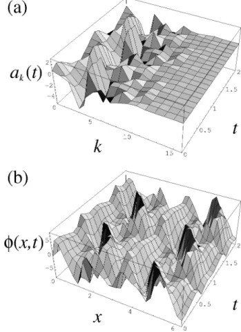
strongly damped and their amplitudes remain very close to zero for all times, but intermediate modes must be kept in the simulations. Figure 2(a) depicts the temporal variation of the Fourier modes ak(t) in Eq. (12) for a chaotic regime

at ν = 0.029919 and N = 16 modes. Clearly, the energy is concentrated in the low-k long wavelength modes. The corresponding spatiotemporal pattern φ(x, t) in real space, obtained with Eq. (5), is shown in Fig. 2(b). The system dynamics is chaotic in time but coherent in space.

4 Nonlinear dynamics analysis 4.1 The bifurcation diagram

Figure 3(a) depicts the bifurcation diagram a6(ν) for Eq.

(12) with N = 16. The diagram is similar for any choice of

ak. For each value of ν we drop the initial 100 iterations of

the Poincar´e map before we start plotting. These initial iter-ations contain the transient dynamics, before the fluctuiter-ations of the wave phase converge to a regime where the Poincar´e points stay in an attracting subset of the phase space. For this range of ν, the attracting set can be either chaotic or pe-riodic. The gray area in Fig. 3(a) depicts another important subset of the phase space representing a chaotic saddle. The

Fig. 2. (a) Temporal variation of the Fourier modes ak(t) in Eq.

(12) for ν = 0.029919 and N = 16 modes; (b) the corresponding spatiotemporal pattern of φ(x, t). The system dynamics is chaotic in time but coherent in space.

trajectories of random initial conditions are first attracted to the vicinity of the chaotic saddle, where they display chaotic behavior for a finite time (chaotic transient), before they con-verge to the attractor (periodic or chaotic). The chaotic sad-dles are obtained by the PIM triple algorithm (Nusse and Yorke, 1989).

A saddle-node bifurcation at ν = νSN B ≈ 0.02992498,

indicated as SNB in Fig. 1, marks the beginning of a

pe-riodic window in the bifurcation diagram. For ν > νSN B,

random initial conditions converge to a chaotic attractor, and for ν < νSN Bthe chaotic attractor no longer exists. At the

saddle-node bifurcation the simultaneous creation of a p-3 attractor and a p-3 unstable periodic orbit occurs. The p-3 UPO, found with the Newton method, is represented in Fig. 3(a) by dashed lines. As the value of ν is decreased, the p-3 attractor undergoes a cascade of period-doubling bifur-cations, whereby the period of the attractor is successively doubled. As the period tends towards infinity, a chaotic at-tractor is formed, localized in three separate bands in the bifurcation diagram. We call the region occupied by this “banded” attractor the band region (B), and the region occu-pied by the surrounding chaotic saddle (SCS) the

surround-Fig. 1. Period-3 limit cycle solution of Eq. (12) at ν=0.029924 and

the corresponding Poincar´e points.

with k=1, ..., N .

The dynamics of the system described by Eq. (12) can be analyzed on a Poincar´e section defined by a1=0. A trajectory

representing the flow of Eq. (12) in a phase space defined by the Fourier modes ak, can intersect this Poincar´e section in

two ways: when ˙a1>0 (from “left” to “right”) or when ˙a1<0

(from “right” to “left”). We adopt a Poincar´e map P de-fined as the (N −1) dimensional hyperplane given by a1=0,

with ˙a1>0, so that a Poincar´e point is plotted every time the

flow of Eq. (12) crosses the Hyperplane a1=0 from “left” to

“right”, as illustrated in Fig. 1 for a period-3 (p-3) limit cycle solution at ν=0.029924.

The choice of the truncation N for the number of modes has obvious implications in the numerical solutions of Eq. (3). High values of N imply high computational cost for the simulations, due to the sums in the nonlinear term in Eq. (12). On the other hand, low values of N may re-sult in a dynamical system whose behavior has no resem-blance with the original PDE. A determination of the range of linearly unstable modes is helpful in this case. Consid-ering the linear part of Eq. (12), one finds that the stability eigenvalues are negative for |k|>1/√ν and are positive for

|k|<1/√ν. Thus, the modes with wave numbers k in the range [−1/√ν,1/√ν]are linearly unstable. These modes excite the short wavelength (high-k) modes through the non-linear term in Eq. (12), and the excitations are dissipated by the high-k modes (Christiansen et al., 1997). Modes with

|k|1/√νare strongly damped and their amplitudes remain very close to zero for all times, but intermediate modes must be kept in the simulations. Figure 2a depicts the tempo-ral variation of the Fourier modes ak(t ) in Eq. (12) for a

chaotic regime at ν=0.029919 and N =16 modes. Clearly, the energy is concentrated in the low-k long wavelength modes. The corresponding spatiotemporal pattern φ (x, t ) in real space, obtained with Eq. (5), is shown in Fig. 2b. The system dynamics is chaotic in time but coherent in space.

4 Rempel et al.: Intermittent chaos driven by nonlinear Alfv´en waves

Fig. 1. Period-3 limit cycle solution of Eq. (12) at ν = 0.029924

and the corresponding Poincar´e points.

the simulations, due to the sums in the nonlinear term in Eq. (12). On the other hand, low values of N may result in a dy-namical system whose behavior has no resemblance with the original PDE. A determination of the range of linearly unsta-ble modes is helpful in this case. Considering the linear part of Eq. (12), one finds that the stability eigenvalues are nega-tive for |k| > 1/√ν and are positive for |k| < 1/√ν. Thus,

the modes with wave numbers k in the range [−1/√ν, 1/√ν]

are linearly unstable. These modes excite the short wave-length (high-k) modes through the nonlinear term in Eq. (12), and the excitations are dissipated by the high-k modes (Christiansen et al., 1997). Modes with |k| 1/√ν are

strongly damped and their amplitudes remain very close to zero for all times, but intermediate modes must be kept in the simulations. Figure 2(a) depicts the temporal variation of the Fourier modes ak(t) in Eq. (12) for a chaotic regime

at ν = 0.029919 and N = 16 modes. Clearly, the energy is concentrated in the low-k long wavelength modes. The corresponding spatiotemporal pattern φ(x, t) in real space, obtained with Eq. (5), is shown in Fig. 2(b). The system dynamics is chaotic in time but coherent in space.

Figure 3(a) depicts the bifurcation diagram a6(ν) for Eq.

(12) with N = 16. The diagram is similar for any choice of

ak. For each value of ν we drop the initial 100 iterations of

the Poincar´e map before we start plotting. These initial iter-ations contain the transient dynamics, before the fluctuiter-ations of the wave phase converge to a regime where the Poincar´e points stay in an attracting subset of the phase space. For this range of ν, the attracting set can be either chaotic or pe-riodic. The gray area in Fig. 3(a) depicts another important subset of the phase space representing a chaotic saddle. The

Fig. 2. (a) Temporal variation of the Fourier modes ak(t) in Eq.

(12) for ν = 0.029919 and N = 16 modes; (b) the corresponding spatiotemporal pattern of φ(x, t). The system dynamics is chaotic in time but coherent in space.

trajectories of random initial conditions are first attracted to the vicinity of the chaotic saddle, where they display chaotic behavior for a finite time (chaotic transient), before they con-verge to the attractor (periodic or chaotic). The chaotic sad-dles are obtained by the PIM triple algorithm (Nusse and Yorke, 1989).

A saddle-node bifurcation at ν = νSN B ≈ 0.02992498,

indicated as SNB in Fig. 1, marks the beginning of a

pe-riodic window in the bifurcation diagram. For ν > νSN B,

random initial conditions converge to a chaotic attractor, and for ν < νSN B the chaotic attractor no longer exists. At the

saddle-node bifurcation the simultaneous creation of a p-3 attractor and a p-3 unstable periodic orbit occurs. The p-3 UPO, found with the Newton method, is represented in Fig. 3(a) by dashed lines. As the value of ν is decreased, the p-3 attractor undergoes a cascade of period-doubling bifur-cations, whereby the period of the attractor is successively doubled. As the period tends towards infinity, a chaotic at-tractor is formed, localized in three separate bands in the bifurcation diagram. We call the region occupied by this “banded” attractor the band region (B), and the region occu-pied by the surrounding chaotic saddle (SCS) the

surround-Fig. 2. (a) Temporal variation of the Fourier modes ak(t )in Eq. (12)

for ν=0.029919 and N =16 modes; (b) the corresponding spa-tiotemporal pattern of φ(x, t ). The system dynamics is chaotic in time but coherent in space.

Figure 3a depicts the bifurcation diagram a6(ν)for Eq. (12)

with N =16. The diagram is similar for any choice of ak.

For each value of ν we drop the initial 100 iterations of the Poincar´e map before we start plotting. These initial iterations contain the transient dynamics, before the fluctuations of the wave phase converge to a regime where the Poincar´e points stay in an attracting subset of the phase space. For this range of ν, the attracting set can be either chaotic or periodic. The gray area in Fig. 3a depicts another important subset of the phase space representing a chaotic saddle. The trajectories of random initial conditions are first attracted to the vicinity of the chaotic saddle, where they display chaotic behavior for a finite time (“chaotic transient”), before they converge to the attractor (periodic or chaotic). The chaotic saddles are obtained by the PIM triple algorithm (Nusse and Yorke, 1989).

A saddle-node bifurcation at ν=νSNB≈0.02992498,

indi-cated as SNB in Fig. 1, marks the beginning of a “peri-odic window” in the bifurcation diagram. For ν>νSNB,

(6)

ran-E. L. Rempel et al.: Intermittent chaos driven by nonlinear Alfv´en wavesRempel et al.: Intermittent chaos driven by nonlinear Alfv´en waves 6955

Fig. 3. (a) Variation of a6for the chaotic saddle (gray) as a

func-tion of ν, superimposed by the bifurcafunc-tion diagram of the attractor (black) in a p-3 periodic window. IC denotes interior crisis and SNB denotes saddle-node bifurcation. The dashed lines denote the p-3 mediating unstable periodic orbit. (b) Same as (a), but depicting the conversion of the three-band weak chaotic attractor into a band chaotic saddle after (to the left of) IC.

ing region (S), following reference (Szab´o et al., 2000). At ν = νIC ≈ 0.02992021 the chaotic attractor collides with

the p-3 UPO created at SNB, called the mediating

unsta-ble periodic orbit (MPO). This collision is responsiunsta-ble for

an interior crisis, which is a sudden enlargement in the size of a chaotic attractor (Grebogi et al., 1983). After crisis

(ν < νIC), we find a new chaotic saddle embedded in the

enlarged chaotic attractor, in the region previously occupied by the “pre-IC” banded chaotic attractor. In contrast with the surrounding chaotic saddle, we call this new chaotic sad-dle the band chaotic sadsad-dle (BCS). Figure 3(b) illustrates the structure of BCS after IC, where the bifurcation diagram for the attractor (black) of Fig. 3(a) is plotted to the right of the IC point and the band chaotic saddle (gray) is plotted to the left of IC. It is important to stress that although in Fig. 3(a) the surrounding chaotic saddle is plotted only between points

Fig. 4. (b) Variation of the maximum Lyapunov exponent λmax

with ν; (c) variation of the correlation length ξ with ν.

SNB and IC, it is actually present in the entire bifurcation di-agram. For ν < νICand ν > νSN B SCS is a subset of the

chaotic attractor.

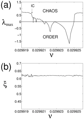
In Fig. 4(a) we plot the variation of the maximum Lya-punov exponent λmaxof the attracting set as a function of

ν. Positive values of λmaxindicate the presence of a chaotic

attractor, and negative values indicate that the attractor is pe-riodic. Note that λmaxjumps abruptly at νIC, indicating a

sudden increase in the attractor’s chaoticity. For that reason, the pre-IC chaotic attractor is called weak chaotic attractor and the post-IC attractor, the strong chaotic attractor. As mentioned before, for the chosen value of the damping pa-rameter ν and the spatial system size L = 2π, the dynamics of the Kuramoto-Sivashinsky equation is chaotic in time, but coherent in space. In fact, the spatial coherence remains basi-cally unaltered throughout the whole range of ν used in Figs. 3 and 4, as indicated by the correlation length ξ (Morris et al., 1993) in Fig. 4(b).

4.2 Chaotic Saddles

Associated to a chaotic saddle, there are stable and unsta-ble manifolds. The staunsta-ble manifold is the set of points that

Fig. 3. (a) Variation of a₆for the chaotic saddle (gray) as a func-tion of ν, superimposed by the bifurcafunc-tion diagram of the attractor (black) in a p-3 periodic window. IC denotes interior crisis and SNB denotes saddle-node bifurcation. The dashed lines denote the p-3 mediating unstable periodic orbit. (b) Same as (a), but depicting the conversion of the three-band weak chaotic attractor into a band chaotic saddle after (to the left of) IC.

dom initial conditions converge to a chaotic attractor, and for

ν<νSNBthe chaotic attractor no longer exists. At the

saddle-node bifurcation the simultaneous creation of a p-3 attractor and a p-3 unstable periodic orbit occurs. The p-3 UPO, found with the Newton method, is represented in Fig. 3a by dashed lines. As the value of ν is decreased, the p-3 attractor under-goes a cascade of period-doubling bifurcations, whereby the period of the attractor is successively doubled. As the period tends towards infinity, a chaotic attractor is formed, local-ized in three separate bands in the bifurcation diagram. We call the region occupied by this “banded” attractor the “band region” (B), and the region occupied by the surrounding chaotic saddle (SCS) the “surrounding region” (S), follow-ing reference (Szab´o et al., 2000). At ν=νIC≈0.02992021

the chaotic attractor collides with the p-3 UPO created at SNB, called the “mediating unstable periodic orbit” (MPO).

Rempel et al.: Intermittent chaos driven by nonlinear Alfv´en waves 5

Fig. 3. (a) Variation of a6for the chaotic saddle (gray) as a

func-tion of ν, superimposed by the bifurcafunc-tion diagram of the attractor (black) in a p-3 periodic window. IC denotes interior crisis and SNB denotes saddle-node bifurcation. The dashed lines denote the p-3 mediating unstable periodic orbit. (b) Same as (a), but depicting the conversion of the three-band weak chaotic attractor into a band chaotic saddle after (to the left of) IC.

ing region (S), following reference (Szab´o et al., 2000). At ν = νIC ≈ 0.02992021 the chaotic attractor collides with

the p-3 UPO created at SNB, called the mediating

unsta-ble periodic orbit (MPO). This collision is responsiunsta-ble for

an interior crisis, which is a sudden enlargement in the size of a chaotic attractor (Grebogi et al., 1983). After crisis

(ν < νIC), we find a new chaotic saddle embedded in the

enlarged chaotic attractor, in the region previously occupied by the “pre-IC” banded chaotic attractor. In contrast with the surrounding chaotic saddle, we call this new chaotic sad-dle the band chaotic sadsad-dle (BCS). Figure 3(b) illustrates the structure of BCS after IC, where the bifurcation diagram for the attractor (black) of Fig. 3(a) is plotted to the right of the IC point and the band chaotic saddle (gray) is plotted to the left of IC. It is important to stress that although in Fig. 3(a) the surrounding chaotic saddle is plotted only between points

Fig. 4. (b) Variation of the maximum Lyapunov exponent λmax

with ν; (c) variation of the correlation length ξ with ν.

SNB and IC, it is actually present in the entire bifurcation di-agram. For ν < νIC and ν > νSN B SCS is a subset of the

chaotic attractor.

In Fig. 4(a) we plot the variation of the maximum Lya-punov exponent λmaxof the attracting set as a function of

ν. Positive values of λmaxindicate the presence of a chaotic

attractor, and negative values indicate that the attractor is pe-riodic. Note that λmax jumps abruptly at νIC, indicating a

sudden increase in the attractor’s chaoticity. For that reason, the pre-IC chaotic attractor is called weak chaotic attractor and the post-IC attractor, the strong chaotic attractor. As mentioned before, for the chosen value of the damping pa-rameter ν and the spatial system size L = 2π, the dynamics of the Kuramoto-Sivashinsky equation is chaotic in time, but coherent in space. In fact, the spatial coherence remains basi-cally unaltered throughout the whole range of ν used in Figs. 3 and 4, as indicated by the correlation length ξ (Morris et al., 1993) in Fig. 4(b).

4.2 Chaotic Saddles

Associated to a chaotic saddle, there are stable and unsta-ble manifolds. The staunsta-ble manifold is the set of points that

Fig. 4. (a) Variation of the maximum Lyapunov exponent λmaxwith

ν; (b) variation of the correlation length ξ with ν.

This collision is responsible for an “interior crisis”, which is a sudden enlargement in the size of a chaotic attractor (Gre-bogi et al., 1983). After crisis (ν<νIC), we find a new chaotic

saddle embedded in the enlarged chaotic attractor, in the re-gion previously occupied by the “pre-IC” banded chaotic at-tractor. In contrast with the surrounding chaotic saddle, we call this new chaotic saddle the “band chaotic saddle” (BCS). Figure 3b illustrates the structure of BCS after IC, where the bifurcation diagram for the attractor (black) of Fig. 3a is plot-ted to the right of the IC point and the band chaotic saddle (gray) is plotted to the left of IC. It is important to stress that although in Fig. 3a the surrounding chaotic saddle is plotted only between points SNB and IC, it is actually present in the entire bifurcation diagram. For ν<νICand ν>νSNBSCS is a

subset of the chaotic attractor.

In Fig. 4a we plot the variation of the maximum Lyapunov exponent λmaxof the attracting set as a function of ν.

Pos-itive values of λmax indicate the presence of a chaotic

at-tractor, and negative values indicate that the attractor is pe-riodic. Note that λmax jumps abruptly at νIC, indicating a

sudden increase in the attractor’s chaoticity. For that reason, the pre-IC chaotic attractor is called “weak chaotic attrac-tor” and the post-IC attractor, the “strong chaotic attracattrac-tor”. As mentioned before, for the chosen value of the damping

(7)

Fig. 5. Transient chaos at ν = 0.0299248.

converge to the chaotic saddle in forward time dynamics; the unstable manifold is the set of points that converge to the chaotic saddle in the time reversed dynamics. The chaotic saddle lies on the intersection of its stable and unstable man-ifolds (Nusse and Yorke, 1989; Ziemniak et al., 1994). In-side the periodic window (between SNB and IC in Fig. 3) the trajectories of all initial conditions will eventually con-verge to an attractor, except for initial conditions lying on the stable manifold of SCS, which is a set of measure zero. Initial conditions close to the stable manifold are first at-tracted to SCS and stay close to its neighborhood for some time, before they are repelled, following its unstable mani-fold. The closer an initial condition is to the stable manifold of SCS, the longer its transient time before converging to the attractor (Hsu et al., 1988). In Fig. 5 an example of tran-sient chaos is shown for a time series of Poincar´e points at

ν = 0.0299248, where the phase dynamics converges to a

p-3 attractor. The average transient time τ can be estimated by taking N0random initial conditions and computing Nt,

the number of trajectories that are still in the transient stage after t iterates. Figure 6 shows a graph of log Nt versus t

at ν = νIC, where N0 = 10000 different initial conditions

were used. The graph can be fitted with a straight line of slope γ = −3.59 × 10−2 ± 1.45 × 10−4_{, which gives an}

average exit time τ = −1/γ ≈ 27.9 (Rempel et al., 2004). Figure 7 shows a three-dimensional projection (a1, a10,

a16) of a chaotic saddle defined in the 15-dimensional

Poincar´e hyperplane at ν = 0.029925 > νSN B, to the right

of the saddle-node bifurcation in Fig. 3(a). This chaotic sad-dle is a continuation of the surrounding chaotic sadsad-dle shown in Fig. 3(a). The chaotic saddle is not a continuous line. It has many gaps, most of which are not visible in Fig. 7 due to their small size.

4.3 Interior crisis

In this section the dynamics near the interior crisis point νIC

is investigated in terms of the role of chaotic saddles and UPOs. For details on the numerical algorithms employed see Rempel and Chian (2003) and Rempel et al. (2004).

Fig. 6. Exponential decay of Nt, the number of trajectories inside

the restraining region at time t, as a function of t. The inverse of the slope of the fitted line gives the average exit time τ ≈ 27.9.

Fig. 7. Three-dimensional projection (a1, a10, a16) of the chaotic

saddle defined in the 15-dimensional Poincar´e hyperplane just be-fore the saddle-node bifurcation, at ν = 0.029925.

At crisis the collision of the mediating UPO with the tree-band weak chaotic attractor at νIC results in the

for-mation of a single-band strong chaotic attractor. Figure 8 shows a three-dimensional projection (a1, a10, a16) of the

Poincar´e points of the strong chaotic attractor (SCA, light line) after crisis (ν = 0.02992006), superimposed by the 3-band weak chaotic attractor (WCA, dark lines) at crisis

(ν = 0.02992021). An estimation of the fractal dimension of

the post-crisis chaotic attractor at ν = 0.02992006 using the Kaplan-Yorke formula (Ott, 1993) results in the dimension

D ≈ 2.08. Note the similarity of the strong chaotic attractor

with the surrounding chaotic saddle shown in Fig. 7. In Fig. 9 we plot a two-dimensional projection (a5, a6) of

the upper branch of the chaotic attractor CA (black line) with the surrounding chaotic saddle SCS (red lines) and its stable manifold (blue dots) for (a) ν = 0.0299211 (before crisis)

Fig. 5. Transient chaos at ν=0.0299248.

parameter ν and the spatial system size L=2π , the dynam-ics of the Kuramoto-Sivashinsky equation is chaotic in time, but coherent in space. In fact, the spatial coherence remains basically unaltered throughout the whole range of ν used in Figs. 3 and 4, as indicated by the correlation length ξ (Morris et al., 1993) in Fig. 4b.

4.2 Chaotic saddles

Associated to a chaotic saddle, there are stable and unsta-ble manifolds. The staunsta-ble manifold is the set of points that converge to the chaotic saddle in forward time dynamics; the unstable manifold is the set of points that converge to the chaotic saddle in the time reversed dynamics. The chaotic saddle lies on the intersection of its stable and unstable man-ifolds (Nusse and Yorke, 1989; Ziemniak et al., 1994). In-side the periodic window (between SNB and IC in Fig. 3) the trajectories of all initial conditions will eventually con-verge to an attractor, except for initial conditions lying on the stable manifold of SCS, which is a set of measure zero. Initial conditions close to the stable manifold are first at-tracted to SCS and stay close to its neighborhood for some time, before they are repelled, following its unstable mani-fold. The closer an initial condition is to the stable manifold of SCS, the longer its transient time before converging to the attractor (Hsu et al., 1988). In Fig. 5 an example of tran-sient chaos is shown for a time series of Poincar´e points at

ν=0.0299248, where the phase dynamics converges to a p-3 attractor. The average transient time τ can be estimated by taking N0 random initial conditions and computing Nt,

at ν=νIC, where N0=10 000 different initial conditions were

used. The graph can be fitted with a straight line of slope

γ =−3.59×10−2±1.45×10−4, which gives an average exit time τ =−1/γ ≈27.9 (Rempel et al., 2004).

Figure 7 shows a three-dimensional projection (a1, a10,

Poincar´e hyperplane at ν=0.029925>νSNB, to the right of

the saddle-node bifurcation in Fig. 3a. This chaotic saddle

6 Rempel et al.: Intermittent chaos driven by nonlinear Alfv´en waves

converge to the chaotic saddle in forward time dynamics; the

unstable manifold is the set of points that converge to the

chaotic saddle in the time reversed dynamics. The chaotic

saddle lies on the intersection of its stable and unstable

man-ifolds (Nusse and Yorke, 1989; Ziemniak et al., 1994).

In-side the periodic window (between SNB and IC in Fig. 3)

the trajectories of all initial conditions will eventually

con-verge to an attractor, except for initial conditions lying on

the stable manifold of SCS, which is a set of measure zero.

Initial conditions close to the stable manifold are first

at-tracted to SCS and stay close to its neighborhood for some

time, before they are repelled, following its unstable

mani-fold. The closer an initial condition is to the stable manifold

of SCS, the longer its transient time before converging to the

attractor (Hsu et al., 1988). In Fig. 5 an example of

tran-sient chaos is shown for a time series of Poincar´e points at

ν = 0.0299248, where the phase dynamics converges to a

p-3 attractor. The average transient time τ can be estimated

by taking N

0

random initial conditions and computing N

t

,

the number of trajectories that are still in the transient stage

after t iterates. Figure 6 shows a graph of log N

t

versus t

at ν = ν

IC

, where N

0

= 10000 different initial conditions

were used. The graph can be fitted with a straight line of

slope γ = −3.59 × 10

−2

± 1.45 × 10

−4

_{, which gives an}

average exit time τ = −1/γ ≈ 27.9 (Rempel et al., 2004).

Figure 7 shows a three-dimensional projection (a

1

, a

10

,

a

16

) of a chaotic saddle defined in the 15-dimensional

Poincar´e hyperplane at ν = 0.029925 > ν

SN B

, to the right

of the saddle-node bifurcation in Fig. 3(a). This chaotic

sad-dle is a continuation of the surrounding chaotic sadsad-dle shown

in Fig. 3(a). The chaotic saddle is not a continuous line. It

has many gaps, most of which are not visible in Fig. 7 due to

their small size.

4.3 Interior crisis

In this section the dynamics near the interior crisis point ν

IC

is investigated in terms of the role of chaotic saddles and

UPOs. For details on the numerical algorithms employed

see Rempel and Chian (2003) and Rempel et al. (2004).

At crisis the collision of the mediating UPO with the

tree-band weak chaotic attractor at ν

IC

results in the

for-mation of a single-band strong chaotic attractor. Figure 8

shows a three-dimensional projection (a

1

, a

10

, a

16

) of the

Poincar´e points of the strong chaotic attractor (SCA, light

line) after crisis (ν = 0.02992006), superimposed by the

3-band weak chaotic attractor (WCA, dark lines) at crisis

(ν = 0.02992021). An estimation of the fractal dimension of

the post-crisis chaotic attractor at ν = 0.02992006 using the

Kaplan-Yorke formula (Ott, 1993) results in the dimension

D ≈ 2.08. Note the similarity of the strong chaotic attractor

with the surrounding chaotic saddle shown in Fig. 7.

In Fig. 9 we plot a two-dimensional projection (a

5

, a

6

) of

the upper branch of the chaotic attractor CA (black line) with

the surrounding chaotic saddle SCS (red lines) and its stable

manifold (blue dots) for (a) ν = 0.0299211 (before crisis)

the restraining region at time t, as a function of t. The inverse of the slope of the fitted line gives the average exit time τ ≈27.9.

converge to the chaotic saddle in forward time dynamics; the unstable manifold is the set of points that converge to the chaotic saddle in the time reversed dynamics. The chaotic saddle lies on the intersection of its stable and unstable man-ifolds (Nusse and Yorke, 1989; Ziemniak et al., 1994). In-side the periodic window (between SNB and IC in Fig. 3) the trajectories of all initial conditions will eventually con-verge to an attractor, except for initial conditions lying on the stable manifold of SCS, which is a set of measure zero. Initial conditions close to the stable manifold are first at-tracted to SCS and stay close to its neighborhood for some time, before they are repelled, following its unstable mani-fold. The closer an initial condition is to the stable manifold of SCS, the longer its transient time before converging to the attractor (Hsu et al., 1988). In Fig. 5 an example of tran-sient chaos is shown for a time series of Poincar´e points at

ν = 0.0299248, where the phase dynamics converges to a

p-3 attractor. The average transient time τ can be estimated by taking N0random initial conditions and computing Nt,

at ν = νIC, where N0 = 10000 different initial conditions

were used. The graph can be fitted with a straight line of slope γ = −3.59 × 10−2 ± 1.45 × 10−4_{, which gives an}

average exit time τ = −1/γ ≈ 27.9 (Rempel et al., 2004). Figure 7 shows a three-dimensional projection (a1, a10,

Poincar´e hyperplane at ν = 0.029925 > νSN B, to the right

of the saddle-node bifurcation in Fig. 3(a). This chaotic sad-dle is a continuation of the surrounding chaotic sadsad-dle shown in Fig. 3(a). The chaotic saddle is not a continuous line. It has many gaps, most of which are not visible in Fig. 7 due to their small size.

4.3 Interior crisis

for-mation of a single-band strong chaotic attractor. Figure 8 shows a three-dimensional projection (a1, a10, a16) of the

Poincar´e points of the strong chaotic attractor (SCA, light line) after crisis (ν = 0.02992006), superimposed by the 3-band weak chaotic attractor (WCA, dark lines) at crisis

(ν = 0.02992021). An estimation of the fractal dimension of

the post-crisis chaotic attractor at ν = 0.02992006 using the Kaplan-Yorke formula (Ott, 1993) results in the dimension

D ≈ 2.08. Note the similarity of the strong chaotic attractor

with the surrounding chaotic saddle shown in Fig. 7. In Fig. 9 we plot a two-dimensional projection (a5, a6) of

the upper branch of the chaotic attractor CA (black line) with the surrounding chaotic saddle SCS (red lines) and its stable manifold (blue dots) for (a) ν = 0.0299211 (before crisis)

Fig. 7. Three-dimensional projection (a₁, a₁₀, a₁₆)of the chaotic saddle defined in the 15-dimensional Poincar´e hyperplane just be-fore the saddle-node bifurcation, at ν=0.029925.

is a continuation of the surrounding chaotic saddle shown in Fig. 3a. The chaotic saddle is not a continuous line. It has many gaps, most of which are not visible in Fig. 7 due to their small size.

4.3 Interior crisis

for-mation of a single-band strong chaotic attractor. Figure 8 shows a three-dimensional projection (a1, a10, a16)of the

(8)

E. L. Rempel et al.: Intermittent chaos driven by nonlinear Alfv´en wavesRempel et al.: Intermittent chaos driven by nonlinear Alfv´en waves 6977

Fig. 8. Three-dimensional projection (a1, a10, a16) of the strong

chaotic attractor (SCA, light line) defined in the 15-dimensional Poincar´e hyperplane after crisis at ν = 0.02992006, superimposed by the three-band weak chaotic attractor (WCA, dark lines) at crisis

(ν = 0.02992021).

and (b) ν = 0.02992021 (at crisis). The upper Poincar´e point of the p-3 mediating orbit is represented by the cross. In the Poincar´e map, an unstable periodic orbit turns into a set of saddle points with their associated stable and unstable man-ifolds. The dashed lines in Fig. 9 denote the local branches of the stable manifold (SM) of the mediating orbit (MPO). Note that SCS has a large gap between the two dashed lines, and many other smaller gaps, or discontinuities. Its gaps are due to the horizontal white spaces in the background, which reflect the fractal structure of the stable manifold of SCS. Figure 9(b) reveals that at crisis the S chaotic saddle and the weak chaotic attractor collide. The collision takes place at the mediating saddle, which belongs to SCS. Likewise, the weak chaotic attractor collides with the stable manifolds of both SCS and MPO.

4.4 Crisis-induced intermittency

After the crisis, it is still possible to determine the B and S regions, which are separated by the stable manifold of MPO. Figure 10 shows the chaotic sets for ν = 0.02992006, af-ter the crisis, around the upper branch of the strong chaotic attractor shown in Fig. 8. Figure 10(a) shows the chaotic attractor (CA) and Fig. 10(b) shows the corresponding B (green lines) and S (red lines) chaotic saddles. BCS is local-ized in a region of the phase space previously occupied by the pre-crisis weak chaotic attractor. SCS is the continuation of the pre-crisis surrounding chaotic saddle. It can be seen from Fig. 10 that the post-crisis B and S chaotic saddles are subsets of the strong chaotic attractor. The gaps in SCS and BCS are filled by a set of coupling UPO’s created at the crisis (Robert et al., 2000).

The two post-IC chaotic saddles are not attracting, but they exert influence on the dynamics of nearby orbits, since they

Fig. 9. Plots of the upper branch of the chaotic attractor (CA,

black line), the surrounding chaotic saddle (SCS, red lines) and its stable manifolds (blue dots): (a) before the interior crisis, at

ν = 0.0299211; and (b) at the interior crisis, ν = 0.02992021.

The cross denotes one of the Poincar´e points of the p-3 mediat-ing unstable periodic orbit. The dashed lines represent segments of the boundary between the band region and the surrounding re-gion, given by the stable manifolds (SM) of the mediating unstable periodic orbit.

are responsible for chaotic transients. For ν > νIC,

trajecto-ries on the chaotic attractor never abandon the band region. For ν slightly less than νICa trajectory started in the B region

can stay in B for a long time, after which it crosses SM and escapes to region S. Once it is in the surrounding region, the trajectory is in the neighborhood of SCS. Since SCS is nonat-tracting, after some time the trajectory is “re-injected” into region B. The “jumps” between regions B and S repeat in-termittently. This crisis-induced intermittency can be viewed as an alternation between two transient behaviors, in which the trajectory spends a finite time in the vicinity of either BCS or SCS. These transitions between regions B and S are due to the coupling UPO’s that are located within the gaps of BCS and SCS, and establish the dynamical connection between the two chaotic saddles (Szab´o et al., 2000; Rem-pel and Chian, 2004). The crisis-induced intermittency is

Fig. 8. Three-dimensional projection (a1, a10, a16)of the strong

chaotic attractor (SCA, light line) defined in the 15-dimensional Poincar´e hyperplane after crisis at ν=0.02992006, superimposed by the three-band weak chaotic attractor (WCA, dark lines) at crisis

(ν=0.02992021).

Poincar´e points of the strong chaotic attractor (SCA, light line) after crisis (ν=0.02992006), superimposed by the 3-band weak chaotic attractor (WCA, dark lines) at crisis

(ν=0.02992021). An estimation of the fractal dimension of the post-crisis chaotic attractor at ν=0.02992006 using the Kaplan-Yorke formula (Ott, 1993) results in the dimension

D≈2.08. Note the similarity of the strong chaotic attractor with the surrounding chaotic saddle shown in Fig. 7.

In Fig. 9 we plot a two-dimensional projection (a5, a6) of

the upper branch of the chaotic attractor CA (black line) with the surrounding chaotic saddle SCS (red lines) and its stable manifold (blue dots) for (a) ν=0.0299211 (before crisis) and (b) ν=0.02992021 (at crisis). The upper Poincar´e point of the p-3 mediating orbit is represented by the cross. In the Poincar´e map, an unstable periodic orbit turns into a set of saddle points with their associated stable and unstable man-ifolds. The dashed lines in Fig. 9 denote the local branches of the stable manifold (SM) of the mediating orbit (MPO). Note that SCS has a large gap between the two dashed lines, and many other smaller gaps, or discontinuities. Its gaps are due to the horizontal white spaces in the background, which reflect the fractal structure of the stable manifold of SCS. Figure 1b reveals that at crisis the S chaotic saddle and the weak chaotic attractor collide. The collision takes place at the mediating saddle, which belongs to SCS. Likewise, the weak chaotic attractor collides with the stable manifolds of both SCS and MPO.

After the crisis, it is still possible to determine the B and S regions, which are separated by the stable manifold of MPO. Figure 10 shows the chaotic sets for ν=0.02992006, after the crisis, around the upper branch of the strong chaotic

attrac-Rempel et al.: Intermittent chaos driven by nonlinear Alfv´en waves 7

Fig. 8. Three-dimensional projection (a1, a10, a16) of the strong

chaotic attractor (SCA, light line) defined in the 15-dimensional Poincar´e hyperplane after crisis at ν = 0.02992006, superimposed by the three-band weak chaotic attractor (WCA, dark lines) at crisis

(ν = 0.02992021).

and (b) ν = 0.02992021 (at crisis). The upper Poincar´e point of the p-3 mediating orbit is represented by the cross. In the Poincar´e map, an unstable periodic orbit turns into a set of saddle points with their associated stable and unstable man-ifolds. The dashed lines in Fig. 9 denote the local branches of the stable manifold (SM) of the mediating orbit (MPO). Note that SCS has a large gap between the two dashed lines, and many other smaller gaps, or discontinuities. Its gaps are due to the horizontal white spaces in the background, which reflect the fractal structure of the stable manifold of SCS. Figure 9(b) reveals that at crisis the S chaotic saddle and the weak chaotic attractor collide. The collision takes place at the mediating saddle, which belongs to SCS. Likewise, the weak chaotic attractor collides with the stable manifolds of both SCS and MPO.

After the crisis, it is still possible to determine the B and S regions, which are separated by the stable manifold of MPO. Figure 10 shows the chaotic sets for ν = 0.02992006, af-ter the crisis, around the upper branch of the strong chaotic attractor shown in Fig. 8. Figure 10(a) shows the chaotic attractor (CA) and Fig. 10(b) shows the corresponding B (green lines) and S (red lines) chaotic saddles. BCS is local-ized in a region of the phase space previously occupied by the pre-crisis weak chaotic attractor. SCS is the continuation of the pre-crisis surrounding chaotic saddle. It can be seen from Fig. 10 that the post-crisis B and S chaotic saddles are subsets of the strong chaotic attractor. The gaps in SCS and BCS are filled by a set of coupling UPO’s created at the crisis (Robert et al., 2000).

The two post-IC chaotic saddles are not attracting, but they exert influence on the dynamics of nearby orbits, since they

black line), the surrounding chaotic saddle (SCS, red lines) and its stable manifolds (blue dots): (a) before the interior crisis, at

ν = 0.0299211; and (b) at the interior crisis, ν = 0.02992021.

The cross denotes one of the Poincar´e points of the p-3 mediat-ing unstable periodic orbit. The dashed lines represent segments of the boundary between the band region and the surrounding re-gion, given by the stable manifolds (SM) of the mediating unstable periodic orbit.

are responsible for chaotic transients. For ν > νIC,

trajecto-ries on the chaotic attractor never abandon the band region. For ν slightly less than νICa trajectory started in the B region

can stay in B for a long time, after which it crosses SM and escapes to region S. Once it is in the surrounding region, the trajectory is in the neighborhood of SCS. Since SCS is nonat-tracting, after some time the trajectory is “re-injected” into region B. The “jumps” between regions B and S repeat in-termittently. This crisis-induced intermittency can be viewed as an alternation between two transient behaviors, in which the trajectory spends a finite time in the vicinity of either BCS or SCS. These transitions between regions B and S are due to the coupling UPO’s that are located within the gaps of BCS and SCS, and establish the dynamical connection between the two chaotic saddles (Szab´o et al., 2000; Rem-pel and Chian, 2004). The crisis-induced intermittency is

black line), the surrounding chaotic saddle (SCS, red lines) and its stable manifolds (blue dots): (a) before the interior crisis, at

ν=0.0299211; and (b) at the interior crisis, ν=0.02992021. The cross denotes one of the Poincar´e points of the p-3 mediating un-stable periodic orbit. The dashed lines represent segments of the boundary between the band region and the surrounding region, given by the stable manifolds (SM) of the mediating unstable pe-riodic orbit.

tor shown in Fig. 8. Figure 10a shows the chaotic attractor (CA) and Fig. 10b shows the corresponding B (green lines) and S (red lines) chaotic saddles. BCS is localized in a re-gion of the phase space previously occupied by the pre-crisis weak chaotic attractor. SCS is the continuation of the pre-crisis surrounding chaotic saddle. It can be seen from Fig. 10 that the post-crisis B and S chaotic saddles are subsets of the strong chaotic attractor. The gaps in SCS and BCS are filled by a set of coupling UPO’s created at the crisis (Robert et al., 2000).

The two post-IC chaotic saddles are not attracting, but they exert influence on the dynamics of nearby orbits, since they are responsible for chaotic transients. For ν>νIC, trajectories

on the chaotic attractor never abandon the band region. For

ν slightly less than νIC a trajectory started in the B region

(9)

Fig. 10. (a) Upper branch of the chaotic attractor (CA) after the

interior crisis, at ν = 0.02992006. The dashed lines indicate seg-ments of the stable manifolds (SM) of the mediating unstable pe-riodic orbit (cross); (b) the band chaotic saddle (BCS, green lines) and the surrounding chaotic saddle (SCS, red lines) that compose the chaotic attractor shown in (a).

characterized by time series containing weakly chaotic lami-nar phases that are randomly interrupted by strongly chaotic bursts, as shown in Fig. 11 for ν = 0.02992. The weakly chaotic laminar phases correspond to the time spent in re-gion B, and the strongly chaotic bursts correspond to the time spent in region S.

The average duration of the “laminar” phases in the inter-mittent time series (the characteristic intermittency time) de-pends on the value of ν. Close to νICthe average time spent

in the vicinity of BCS is very long, and decreases as ν is decreased away from νIC. The characteristic intermittency

time (denoted by τ ) can be obtained as the average over a long time series of the time between switches among regions B and S. Figure 12 is a plot of log₁₀τ vs log10(νIC − ν),

where the solid line with slope γ ≈ −0.46 is a linear fit of the values of the characteristic intermittency time com-puted from time series (circles). Figure 12 reveals that the characteristic time τ decreases with the distance from the critical parameter value νIC following a power-law decay,

Fig. 11. Crisis-induced intermittency at ν = 0.02992.

Fig. 12. log₁₀τ vs log₁₀(νIC− ν). The solid line with slope γ ≈

−0.46 is a linear fit of the values of the characteristic intermittency

time τ computed from time series (circles).

τ ∼ (νIC− ν)γ, as expected (Grebogi et al., 1987a).

5 Conclusions

We have investigated the relevance of chaotic saddles and unstable periodic orbits at the onset of intermittent chaos in the phase dynamics of nonlinear Alfv´en waves by using the Kuramoto-Sivashinsky equation as a model equation. We de-scribed how a strong chaotic attractor formed after an in-terior crisis can be naturally decomposed into two nonat-tracting chaotic sets, known as chaotic saddles, dynamically linked by a set of coupling unstable periodic orbits. The per-turbed wave phase oscillates irregularly, switching intermit-tently from the neighborhood of one nonattracting chaotic set to the other.

The dynamical scenario described in this paper reflects a situation of intermittency in chaotic spatiotemporal systems that is still distant from the well-developed turbulent regimes

inte-rior crisis, at ν=0.02992006. The dashed lines indicate segments of the stable manifolds (SM) of the mediating unstable periodic orbit (cross); (b) the band chaotic saddle (BCS, green lines) and the sur-rounding chaotic saddle (SCS, red lines) that compose the chaotic attractor shown in (a).

escapes to region S. Once it is in the surrounding region, the trajectory is in the neighborhood of SCS. Since SCS is nonat-tracting, after some time the trajectory is “re-injected” into region B. The “jumps” between regions B and S repeat in-termittently. This crisis-induced intermittency can be viewed as an alternation between two transient behaviors, in which the trajectory spends a finite time in the vicinity of either BCS or SCS. These transitions between regions B and S are due to the coupling UPO’s that are located within the gaps of BCS and SCS, and establish the dynamical connection between the two chaotic saddles (Szab´o et al., 2000; Rem-pel and Chian, 2004). The crisis-induced intermittency is characterized by time series containing weakly chaotic lami-nar phases that are randomly interrupted by strongly chaotic bursts, as shown in Fig. 11 for ν = 0.02992. The weakly chaotic laminar phases correspond to the time spent in re-gion B, and the strongly chaotic bursts correspond to the time spent in region S.

The average duration of the “laminar” phases in the

inter-8 Rempel et al.: Intermittent chaos driven by nonlinear Alfv´en waves

The average duration of the “laminar” phases in the inter-mittent time series (the characteristic intermittency time) de-pends on the value of ν. Close to νICthe average time spent

time (denoted by τ ) can be obtained as the average over a long time series of the time between switches among regions B and S. Figure 12 is a plot of log10τ vs log10(νIC− ν),

Fig. 12. log10τ vs log10(νIC− ν). The solid line with slope γ ≈

5 Conclusions

Fig. 11. Crisis-induced intermittency at ν=0.02992.

The average duration of the “laminar” phases in the inter-mittent time series (the characteristic intermittency time) de-pends on the value of ν. Close to νIC the average time spent

time (denoted by τ ) can be obtained as the average over a long time series of the time between switches among regions B and S. Figure 12 is a plot of log₁₀τ vs log₁₀(νIC − ν),

Fig. 12. log₁₀τ vs log10(νIC− ν). The solid line with slope γ ≈

5 Conclusions

Fig. 12. log₁₀τ vs. log₁₀(νIC−ν). The solid line with slope

γ ≈−0.46 is a linear fit of the values of the characteristic intermit-tency time τ computed from time series (circles).

mittent time series (the “characteristic intermittency time”) depends on the value of ν. Close to νICthe average time spent

in the vicinity of BCS is very long, and decreases as ν is de-creased away from νIC. The characteristic intermittency time

(denoted by τ ) can be obtained as the average over a long time series of the time between switches among regions B and S. Figure 12 is a plot of log₁₀τ vs. log₁₀(νIC−ν), where

the solid line with slope γ ≈−0.46 is a linear fit of the val-ues of the characteristic intermittency time computed from time series (circles). Figure 12 reveals that the characteristic time τ decreases with the distance from the critical parame-ter value νIC following a power-law decay, τ ∼(νIC−ν)γ, as