HAL Id: hal-00385028
https://hal.archives-ouvertes.fr/hal-00385028
Submitted on 14 Feb 2017
HAL is a multi-disciplinary open access
archive for the deposit and dissemination of
sci-entific research documents, whether they are
pub-lished or not. The documents may come from
L’archive ouverte pluridisciplinaire HAL, est
destinée au dépôt et à la diffusion de documents
scientifiques de niveau recherche, publiés ou non,
émanant des établissements d’enseignement et de
Automatic Detection of Instruments in Laparoscopic
Images: A First Step Towards High-level Command of
Robotic Endoscopic Holders
Sandrine Voros, Jean-Alexandre Long, Philippe Cinquin
To cite this version:
Sandrine Voros, Jean-Alexandre Long, Philippe Cinquin. Automatic Detection of Instruments in
Laparoscopic Images: A First Step Towards High-level Command of Robotic Endoscopic Holders.
The International Journal of Robotics Research, SAGE Publications, 2007, 26 (11-12), pp.1173-1190.
�10.1177/0278364907083395�. �hal-00385028�
Automatic detection of instruments in
laparoscopic images: a first step towards high
level command of robotic endoscopic holders
Sandrine Voros
1, Jean-Alexandre Long
2, Philippe Cinquin
1 1Universit´
e J. Fourier, Laboratoire TIMC-IMAG;
CNRS, UMR 5525; INSERM, IFR 130
F-38000 Grenoble, France
{Sandrine.Voros, Philippe.Cinquin}@imag.fr
2
Department of Urology, University Hospital, Grenoble
Abstract
The tracking of surgical instruments offers interesting possibilities for the development of high level commands for robotic camera holders in laparoscopic surgery. We have developed a new method to detect instru-ments in laparoscopic images which uses information on the 3D position of the insertion point of an instrument in the abdominal cavity. This information strongly constrains the search for the instrument in each en-doscopic image. Hence, the instrument can be detected in near real-time using shape considerations. Early results on laparoscopic images show that the method is rapid and robust in the presence of partial occlusion and smoke. Our first experiment on a cadaver validates our approach and shows encouraging results.
keywords: Laparoscopic surgery, Tool tracking, Vision-based control
1
Introduction
Laparoscopic interventions are minimally invasive procedures of the abdominal cavity which are performed with the assistance of a camera and long, thin instruments. Small incisions (usually 1cm) are made, and the abdominal cavity is insuflated with gas in order to create enough space to move the camera and instruments. Tubes called trocars are placed through the incisions to seal the opening and insert the endoscopic camera and the instruments. The surgeon performs the surgical procedure while an assistant holds the endoscopic camera. This type of minimally invasive intervention is less traumatizing for the pa-tient than open surgery: less blood loss, less transfusions, a smaller consumption of anagelsia and a shorter hospitalization time [1]. However, laparoscopic proce-dures are more complex to perform for the surgeon and require experience: the surgeon must use 2D images to perform the procedure, which implies a loss of
depth information. He uses specific instruments which are more difficult to ma-nipulate than conventional instruments. Moreover, a second surgeon is needed for the manipulation of the camera; the coordination between the surgeon and the assistant can be difficult and the images from the endoscopic camera are not stable.
Several medical robots have been developed for the manipulation of the camera. The most popular are Aesop (Computer Motion) and EndoAssistR R
(Armstrong Healthcare) [2]. They enhance the quality of the images [3], reduce the staining of the endoscope, and enable solo surgery since they can be con-trolled by the surgeon by means such as a vocal command or head movement [4], [5]. The main obstacles to the diffusion of such systems in hospitals are their cost, their bulkiness, and the installation time. Moreover, the interaction between the surgeon and the camera holder remains limited (e. g.: left, right, up, down, zoom in and zoom out). The system Aesop offers the possibilityR
to save positions of the robotic arm in order to automatically reposition the endoscope, but due to the passive wrist architecture of the robot, the reposi-tionning is not accurate [6]. To address this problem, Munoz et al. developed an adaptative motion control scheme to compensate the positionning errors of a passive-wrist camera holder [7]. These limits also led to the development of robotic camera holders more adapted to the surgical environment such as the body-mounted robot LER (see section 2).
The development of high level commands for robotic endoscopic holders based on the visual of instruments would be of major clinical added value, since it would allow the surgeon to concentrate on the surgical procedure rather than the control of the robot. A few examples of possible tracking strategies are shown in Fig. 1 :
∗ in [12] Casals et al. present two strategies when two instruments are in the image : if the two instruments are “active”, the tracked point is the middle of the segment defined by the two instruments’ tips. If one instrument is steady, the tracked point also lies on the segment defined by the two tips, but is closer to the moving instrument.
On the contrary to visual-servoing systems, for which the objective is to automatically move a surgical instrument [10], we do not need to localize and track very precisely the surgical instruments, in order to develop the strategies presented in Fig. 1. The main challenge is to retrieve information about each instrument in the laparoscopic image, with as few modifications as possible of surgical protocol or surgical instruments.
Several approaches have been proposed in the literature to deal with this problem. Krupa et al. [10] have designed an instrument holder equipped with a laser beam which projects a pattern on the surface of the organs, allowing the system to safely bring the instrument to a desired location. This approach allows the use of simple, robust, and quick image analysis routines but raises cost issues and adds to the complexity of the laparoscopic set-up. [16] also worked with an instrument holder (a DaVinci system [17]) and used kine-R
matic information and template images of the instruments to detect them in stereo images. This approach requires a robotic instrument holder and implies the use of a limited set of instruments. Wei et al. [11] have designed a color mark fixed on the instrument and use color information to track it with a stereo-scopic laparoscope. Their method is robust in the presence of partial occlusion and blood projection, but it requires to equip all the instruments with marks and raises sterilization issues. Rather than using color information, Casals et al. [12] and Tonet et al. [9] localized a color mark in 3D fixed on an instru-ment with a monoscopic laparoscope using line detection algorithms. The main drawbacks of the approaches based on the use of artificial marks are that they add constraints and complexity to the laparoscopic procedure; each instrument has to be equipped with a mark, raising the question of sterilization. Moreover, when color information is used to detect the marks, the segmentation of the markers has to be robust to variations in illumination. Wang et al. [13] used color classification to detect the instruments among organs but the computation time has not been indicated although it is an issue for a smooth tracking. More recently, Doignon et al. [14] defined a new color purity component that was used to robustly detect instruments in laparoscopic images. Their approach works at half the video rate, but is adapted to gray or metallic instruments only, although some standard laparoscopic instruments have colored shafts. Finally, [15] pro-posed an approach based on the detection of the lines in the image which did not require a color mark, but some parameters have to be tuned manually by the user, which can hardly be envisioned in the context of laparoscopic surgery. It must also be noted that amongst these approaches, the only one that enables the surgeon to identify the instrument he wishes to track is the use of a color mark with a different color for each instrument.
In this article, we present a method to detect the instruments which requires no artificial marker. It uses information on the 3D position of the insertion point of an instrument in the abdominal cavity to detect the latter using shape con-siderations. With an approach based on the shape of the instruments rather than their color, any standard laparoscopic instrument can be detected, what-ever its color. The originality of this method is that knowing the position of the insertion point of an instrument strongly reduces the possible location of the instrument in the endoscopic images. Thus, it can be searched using only image processing in near real time. Moreover, selecting an insertion point allows the user to choose the instrument to track.
Our primary objective is to detect the axis of the instrument; as stated in Fig. 1, when several instruments are visible in the image, the intersection of their axes gives information about the area of interest in the image. This information is sufficient to move the endoscope such that the area of interest is roughly centered in the image. Our secondary objective is to detect the tip of the instrument. This information allows us to keep the tip of an instrument roughly in the center of the image, or to develop tracking strategies for the tracking of several instruments (Fig. 1). For this purpose, we do not require subpixel precision but rather need to roughly determine the position of the tip. A last objective is to detect the edges of the instrument in order obtain information about the distance between the tip of an instrument and the camera, as described in [9]. This allows us to control the zoom of the camera as well as its orientation.
Early results on laparoscopic images show that our detection method is quick and robust in the presence of partial occlusion and smoke, with sufficient preci-sion for the objective of controlling the movements of a robotic camera holder. Our first cadaver test, during which we tracked the tip on one instrument, further proves the feasibility of the approach and allowed us to determine the improvements that are required to comply with real clinical conditions.
2
Material
We work with a three degrees of freedom camera holder prototype (the Light Endoscopic Robot, LER) developed by Berkelman et al. [18]. The LER is a lightweight robot (625 grs. without the camera and the endoscope) which can be directly positioned on the abdomen of the patient, as illustrated by Fig. 2.
a) b)
Figure 2: a) the LER mounted on a cadaver, b) degrees of freedom of the LER.
The robot is controlled by a mini-joystick (Fig. 2) or a vocal command which can be activated or stopped with a dead-man switch. When the surgeon releases his foot from the switch, the microphone is muted and the movement of the robot is interrupted. Simple commands (move left, right, etc.) have been integrated to a control application. New commands can easily be added to the application.
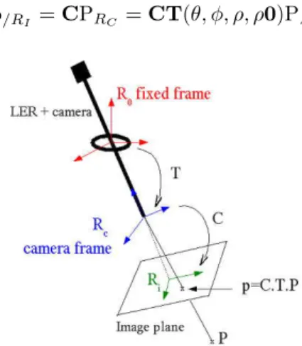
The LER and the endoscopic camera were calibrated using OpenCV library [20] in order to use the robotic system to measure the 3D positions of the inser-tion points of the instruments (see secinser-tion 3.1). The intrinsic calibrainser-tion of the camera was performed using a standard calibration method with a calibration grid [21]. It provided the transformation C linking the 3D coordinates of a point expressed in the camera frame RC to its 2D coordinates in the image frame RI
(see Fig. 3) :
p/RI = CPRC
Since the position of the camera frame varies with time, an extrinsic cali-bration was performed in order to obtain a rough estimation of the rigid trans-formation T between the camera frame RC and a fixed frame linked to the
robot, for a position of reference of the robot. We defined the origin of the fixed frame R0 as the intersection of the two rotation axes of the robot. One of
the axes of R0 is normal to the base plane of the LER and the two other axes
belong to the base plane of the LER. We defined the end-effector frame as the spherical-coordinates frame centered on the tip of the endoscope, and assumed that the camera frame RCand the end-effector frame were superposed (see Fig.
3). With this approximation, we only needed to estimate roughly the distance ρ0 of the tip of the endoscope to the origin of R0 for the reference position of
the LER, in order to compute the rigid transformation T(θ, φ, ρ, ρ0) between RCand R0, for any position of the endoscope. The measurement of ρ0 was done
once, with an optical localizer. This is of course a rough approximation, but as explained in section 1, we do not require a sub-pixel precision for our objectives. We will also explain further on how the instrument detection method deals with calibration uncertainties.
Once the system is calibrated, the 2D coordinates of a point in the endoscopic image can be computed using its 3D coordinates in the fixed frame linked to the robot :
p/RI = CPRC = CT(θ, φ, ρ, ρ0)PR0
Figure 3: Calibrated system: if the coordinates of P are known in R0, its
pro-jection on the image plane can be computed thanks to the calibration matrices T (geometric model of the robot) and C (pinhole model of the camera).
3
Method
In this section, we first present how the 3D positions of the insertion points of the instruments are computed. Then we describe our simple shape model of a laparoscopic instrument. Finally, we explain how, using this information, we find the axis of an instrument, its tip, and its edges. The general framework of the algorithm is presented in 4. In an initialization phase, the surgeon measures the 3D positions of the insertion points with the LER (see section 3.1). In order to track an instrument, the surgeon selects it using its insertion point. The 3D position of the insertion point is projected on the image plane to constrain the search for the instrument in the image (sections 3.2 to 3.6).
Figure 4: Diagram of the different steps of the tracking framework. In this article we focused on the presentation of the instrument detection method (gray block).
3.1
Measurement of the 3D positions of the insertion points
of the instruments
The 3D positions of the insertion points of the instrument are measured at the beginning of the intervention. Since the surgeon gives orders to the robot with a vocal command, we have developed a ‘vocal mouse’ which allows the user to move a cursor on the endoscopic image. For two different positions of the camera in which the insertion point is visible, the surgeon selects the position of the insertion point in the image with the vocal mouse. Using the calibration phase (section 2), we can compute for each position of the camera the projective
line which passes through the insertion point. By calculating the intersection of the two projective lines (or the point in space for which the distance between the two lines is minimal), we obtain the 3D coordinates of the insertion point in the robot frame.
This initialization step could be easily integrated into the surgical protocol since the surgeon creates the insertion points at the beginning of the interven-tion under visual control: for security reasons, when the surgeon makes the incisions on the abdominal wall, he must position the camera so that he sees his instrument entering the abdominal cavity. Recently, Doignon et al. presented an alternative method in which they used a sequence of instrument motions observed by a stationnary camera to find the insertion point of an instrument [22].
We show in section 4 our measurements of the 3D position of an insertion point. The hypothesis that the insertion points are relatively fixed during an intervention is validated.
3.2
Simple shape model of an instrument in laparoscopic
images
The shaft of a laparoscopic instrument has a cylindrical shape, and if we define P = proj(T ) as the projection of an insertion point T in the image plane of the camera, an instrument can be represented in an image by the following elements (Fig. 5):
• three lines: a symmetry axis ∆, and two edges which are symmetrical compared to ∆. The positions of these three lines are constrained by the position of P : C is a circle centered on P of radius R such that the symmetry axis and the two edges intersect C ;
• a point S, which represents the tip of the instrument. S must belong to ∆.
Figure 5: Representation of the instruments in a laparoscopic image. The po-sition of each instrument in the image is constrained by the popo-sition of the projection of its insertion point in the abdominal cavity.
It must be noted that since we use a pinhole model [23] for the camera, we perform a central projection, which does not conserve distances. Thus, the symmetry axis ∆ is not the projection of the symmetry axis of the tool. Moreover, a precise computation of the distance between each edge and P = proj(T ) would require us to project the cylinder representing the instrument on the image for all its (unknown) possible orientations.
Rather than performing these computations, we decided to constrain the position of symmetry axis and the edges using the circle C centered on P of radius R. Since the diameter d of a laparoscopic instrument is known (usually 6 mm), we bounded the value of R from above by the diameter d0 (in pixels)
that the tool would have in the image if it was parallel to the image plane. To validate this choice, we performed a simulation with the Scilab software [24]. We modelled the abdominal cavity as a half sphere, the instrument as a cylinder, and we used the calibration parameters of the camera to model the camera. The insertion point of the endoscope was fixed on the top of the half sphere. We positioned the insertion point of the instrument on the surface of the half-sphere, and the camera inside the half-sphere (Fig. 6). For each position of the insertion point, for each position of the camera, and for each orientation of the instrument, we computed the projections P of the insertion point and of the two edges of the instrument on the image plane (two lines). This allowed us to compute the distance between each edge and P , and thus check that our majoration was correct (Fig. 7).
In order to take into account the uncertainties in the calibration parameters and small movements of the insertion point, it is possible to increase the value of R.
Figure 6: Model of the abdominal cavity, camera and instrument.
Figure 7: Results of the simulation. Color-scale representation of R depending on the position of the instrument on the abdominal wall.
3.3
Step 1 - Search for points belonging to the instrument
In this step, we search for points that are likely to belong to the lines (l1 and l2) representing the edges of the instrument. These points are edges, and the orientation of their gradients is constrained by the position of P (see Fig. 8).
To extract the edges, we use a gradient method where we compute the gradient for each point of the image on each color plane. We keep the maximum of the three gradients, which gives importance to the discontinuities in the image, and store the norm and orientation of the maximum. Points where the gradient is maximum are defined as edges.
We then exploit information about the orientation of the gradient to remove several edge points that cannot correspond to the instrument; an edge point I can belong to the lines representing the edges of the instrument only if its gradient meets the constraints of section III. A: I lies in a zone characterised by the position of P = proj(T ) as illustrated by Fig. 8:
Figure 8: edge detection constrained by the position of the insertion point. In the top figure, the orientation of the gradient is such that the edge point might correspond to the edge of the instrument. In the bottom figure, the orientation is such that the edge point cannot correspond to the instrument.
In other terms, an edge point I of gradient G(x, y) can belong to l1 or l2 only if:
cot(ϕmin) <= GxGy <= cot(ϕmax), where ϕmax= −ϕmin= arccos(kIP kR )
After this process, we obtain a list of points, many of which correspond to the tool. We refine this segmentation process by keeping only the points whose gradient norm is above a threshold (mean norm of the candidate points). We also remove isolated points (simple mask) (see Fig. 9):
a) b)
c) d)
Figure 9: a) Original image, b) segmentation without refinement, c) segmenta-tion with threshold d) threshold and removal of isolated points.
In this step, we have extracted, among all the edge points, those which respect our constraints (later called candidate points). In the next steps, these points are processed in order to find the axis, the tip, and the edges of the instrument.
3.4
Step 2 - Search for the orientation of the instrument
We use the candidate points provided by the previous section to detect the axis using a Hough method [25] that we adapted to our problem to accelerate the computation time.
In 2D, a line can either be described by its cartesian equation y = ax + b or by a point (ρ, θ) in Hough Space, with the relationship ρ = x cos(θ) + y sin θ. ρ is the distance of the line to the origin O and θ is the angle of the line (Fig. 10):
To implement this method for the search of straight lines in an image, a preliminary step consists of finding the edge points in the image. Each edge point in the image votes for a set of parameters (ρ, θ). After this process, the couples (ρ, θ) with the highest votes correspond to lines in the image.
One of the limitations of this method is its computational time. With the conventional Hough method, the origin O of the Hough method (Fig. 10) is usually the center of the image. Thus, if no assumption is made about the orientation of the lines in the image, the parameter θ varies in the interval [0, 2π] and the parameter ρ varies in the interval [0, image diagonal/2].
In order to achieve reasonable computation time, we have shifted the origin to P , the projection of the insertion point (Fig. 11), so that we can reduce the interval of variation of the parameter ρ of the Hough method to [0, R]. The choice of P as the center of the Hough method also makes it possible to reject lines that correspond to instruments in the endoscopic image other than the one inserted through T.
We use the candidate points of the previous step to find a set of points that correspond to a symmetry axis: if two candidate points I1 and I2 have gradients of opposite directions (negative scalar product), I1 can belong to one edge of the instrument, and I2 to the other. For each couple (I1,I2) of candidate points respecting this constraint, we compute the right bisector, characterized by one point (the middle of [I1,I2]) and a direction (the normal of [I1,I2]). If the direction doesn’t meet the orientation constraints of step 1, it cannot correspond to the symmetry axis of the instrument in the image. Otherwise, we characterize the right bisector in Hough space (Fig. 11). Once all the candidate points have been processed, the couple (ρ,θ) which obtains most votes corresponds to the axis of the instrument (Fig. 12).
Figure 11: Hough method centered on the projection of the insertion point of an instrument in the image plane. In this figure, the two edge points I1 and I2 of
gradients G1and G2provide the candidate axis d. This axis is characterized by
the two parameters θ and ρ of a Hough method centered on P , the projection of the insertion point.
a) b)
Figure 12: a) Original image, b) Result of the detection of the axis of the instrument. The yellow dots correspond to the candidate points which voted for the axis.
Knowing the orientation of an instrument is useful, but not sufficient to achieve its tracking. We also need to know the position of its tip to position the camera in the right direction. If we want to include the zoom in the visual servoing of the camera, we can also detect the edges of the instrument to obtain depth information.
3.5
Step 3 - Search for the tip of the instrument
The tip of the instrument is detected using color information: an Otsu threshold ([26]) is applied to the points of the symmetry axis and separates the points of the line into two classes (A and B), one corresponding to the instrument, the other to the background (Fig. 13). The Otsu threshold separates the points of the axis in order to create two classes of points with the maximum variance. Since we have color images, we used the color norm instead of the gray level to compute the Otsu threshold. The pixels belonging to the axis are then studied, starting with the point in the image which is the closest to the insertion point; adjacent points of the same class are grouped in a zone characterized by its starting pixel, its ending pixel, its average color norm, its length, and its class.
Next, we determine which class (A or B) corresponds to the instrument. Our first approach was to find the longest zone of class A and the longest zone of class B and to assume that the zone which is the closest to P = proj(T ) corresponded to the instrument. In Fig. 14, only the longest zone of each class is drawn on the image. Since the insertion point of the instrument is on the right side of the image, the green zone corresponds to the instrument whereas the blue zone corresponds to the background. However, if the instrument is partially occluded, or if there are specular reflections on the instrument, this method can fail.
Figure 14: Longest zone corresponding to the instrument (green) and longest zone corresponding to the background (blue).
We thus decided to use this approach only on the first image (if the de-tection fails, the surgeon can easily interrupt the tracking). The average color norm of the zone corresponding to the instrument (toolColor ), and the average color norm of the zone corresponding to the background (backgroundColor ) are memorized for the next images. In the next images, we also find the longest zone of class A and the longest zone of class B, but this time, the class of the zone whose color norm is closest to toolColor corresponds to the instrument. We define instrumentZone as the longest zone corresponding to the instrument, and backgroundZone as the one corresponding to the background.
Since the zone corresponding to the instrument might not cover the whole length of the instrument (again because of specularities or occlusions), we con-catenate adjacent zones of the same class according to color information. While a zone corresponding to the class of the instrument which is between instrument-Zone and backgroundinstrument-Zone has an average color norm which is closer to toolColor than backgroundColor, we increase the length of the instrument. Finally, the ending pixel of instrumentZone corresponds to the tip of the instrument. Fig. 15 shows the detected tip after this process.
a) b)
Figure 15: a) Original image, b) Tip of the instrument found by the method after the complete process.
3.6
Step 4 - Search for the two edge lines of the instrument
To include the zoom in a visual servoing loop, we can estimate the distance between the camera and the tip of the instrument by analyzing the edges of the instrument in the image (the candidate points obtained in step 1), as suggested by Tonet et al. in [9]. In 3D, since the shaft of the instrument is a cylinder, the angle between the two edges in the image provides information about the depth of the tip (if the angle is null, the tool is parallel to the image plane; if it is positive, the tip is closer to the image plane than the insertion point; if it is negative, the insertion point is closer). More complex techniques such as [19] could also be investigated to find the depth of the tip of the instrument.
The candidate points are separated into two classes: those above the sym-metry axis found in the previous section, and those below. We compute the symmetric of one of the group of points with respect to the symmetry axis to obtain a larger group of points. The line that best fits the points corresponds to one of the edges, and its symmetric with respect to the symmetry axis cor-responds to the other edge.
a) b)
Figure 16: a) Original image, b) Edges of the instrument found by the method after the complete process. The yellow dots correspond to the points which voted for the two edges (after the symmetry computation).
4
Results
This method was implemented with OpenCV library [OpenCV] on a Pentium IV (2.6 GHz, 512 MO RAM) computer. It was first tested on endoscopic images (size 200x100) taken from numerized videos of laparoscopic interventions and cadaver tests to validate the image processing. Then, a visual servoing of our robotic camera holder was developed. At this time, only the orientation of the camera is controlled. The images displayed on the monitor are acquired at a resolution of 720x576 pixels, but the resolution of the input images for the method was reduced to 200x100 to enhance the speed. Since we are not looking for subpixel precision to control the camera (see section 1), a 200x100 resolution is enough for the tracking of a laparoscopic instrument. When we tracked an instrument with the LER, we considered that as long as the distance in the 200x100 image between the tool and the center of the image was greater than 11 pixels, the tool was not centered. Once it was centered, as long as the distance between the tip in the image and the center of the image did not exceed 21 pixels, the tracking was paused. Our objective is to find the tip of a tool in the image with a precision of 11 pixels.
4.1
Results on endoscopic images
This section presents the results we obtained when we tested the method on images taken from numerized videos of laparoscopic procedure. It allowed us to validate our image processing, before developing the complete system with the LER.
For each endoscopic image, we selected with the mouse cursor the entry point P (and the radius R of the circle C) for each instrument we wished to detect. The value of the radius R of the circle C was chosen so it satisfies our tool model (see Fig. 5). As Fig. 17 illustrates, the entry point can be selected in the image plane, and not in the endoscopic image itself (the entry point of an instrument is rarely visible in the image). The computation time is around 100 ms.
Figure 17: Illustration of the selection of the insertion point of an instrument.
In the following figure, we applied the method to different images with in-struments of different colors:
Figure 18: Detection of instruments of different colors: the blue instrument was detected in 93 ms and the black instrument was detected in 94 ms. This shows that the method can apply for instruments of different colors.
If we compare the 2D position of the tip given by the method to the 2D position of the tip manually identified in the image, we obtain an error of 10 pixels for the blue tool and 7 pixels for the black tool, which is sufficient for the visual servoing of the camera, which is enough considering our precision objectives. The detection of the edges is also visually satisfying, but we need to implement a visual servoing of the zoom to determine the precision needed to control the depth of the camera.
We also tested the method on images which contained several instruments (Fig. 19). The instrument to be tracked is selected by choosing an insertion point.
Figure 19: Detection the instruments when several instruments are in the image (first tool detected in 94 ms and second tool in 109 ms).
To a certain extent, the method is also robust to smoke (Fig. 20). In both cases, the axis and edges of the tool are detected correctly; however, the tip of the tool is wrong in the second image because the smoke is too dominant (the Otsu threshold detects the smoke, not the background).
Figure 20: Detection of tools with smoke in the image (125 and 94 ms).
We were also able to identify the problematic cases that must still be solved: in Fig. 21, the tools are nearly aligned, so the method fails in detecting the gray one and the axis found by the method is an average of the axes of both tools.
a)
b) c)
Figure 21: a) Original image, b) detection of the black tool (109 ms), c) the detection of the metallic tool fails (the two tools are nearly aligned).
In Fig. 22 b), the blue tool is detected correctly although its axis intersects the axis of the metallic tool. The specular reflections on the metallic tool cause the failure of the detection of the tip, because the non-shiny parts of the tool have a color closer to the background than to the shiny parts of the tool (Fig. 22. c)). However, if we suppose that in a first image, the tool and background were detected correctly (section 3.5, detection of the tip of the instrument), the results are improved (Fig. 22. d)). In both cases, we can see that the detection of the edges of the metallic tool is not very satisfactory because the specular areas are detected rather than the tip.
a) b)
c) d)
Figure 22: a) Original image, b) detection of the blue tool (125 ms) c) detection of the metallic tool if the image is the first of the sequence (109 ms), d) improved detection if the image is not the first of the sequence (the average color of the tool and background are known).
Finally, Fig. 23 illustrates the most difficult cases still to be solved. For the three instruments, the axes are detected correctly. Again, the difficulty is to detect the tip; for the blue tool (Fig. 23 c)), the metallic tip intersects the tip of another tool, which is also metallic. The metallic tool (Fig. 23 d)) is partially occluded and intersects a black tool. The detection of the tip fails because the color of the tool is assumed to be black.
a) b)
c) d)
Figure 23: a) Original image, b) detection of the black tool c) detection of the blue tool, d) detection of the metallic tool. When the axes intersect, the detection of the tip is difficult.
4.2
Results on anatomical pieces
After this preliminary validation of the feasibility of the method, we imple-mented a visual servoing of the LER (the control of the zoom is not yet included) and tested the full system on a cadaver to simulate clinical conditions.
First, we tested our hypothesis that the insertion points are fixed during the intervention. The results are presented in 4.2.1. We do not take the breathing motion into account, but since the abdominal cavity of the patient is insuflated with gas during the intervention, we can assume that the motion of the insertion point due to breathing is very limited.
We then studied the results of the tracking of an instrument. We observed that the specular reflections needed to be limited for the detection of an instru-ment to be successful and we explain in the discussion how we plan on dealing with this problem. The result of a successful tracking are presented in section 4.2.2.
Finally, we analysed the images for which the detection failed in order to estimate the difficult situations. This error analysis is presented in section 4.2.3 4.2.1 Can the insertion points be considered as fixed?
We measured the position of the insertion point through time using the method presented in subsection 3.1. To check that our first computation was correct, we reprojected the insertion point in an image where the trocart is visible (Fig. 24).
The distance between the measured points and the reference was inferior to 5mm except for measure n˚3, but this was due to leak in of gas in the abdominal cavity. As soon as the leak was stopped the results were satisfying.
n◦ time (min) X (mm) Y (mm) Z (mm) distance (mm) 1 0 78.9 148.4 -39.3 reference 2 11 79.2 152.3 -42.3 1.53 3 14 91.6 207 -39.8 57.3 4 25 71.3 143.5 -52.3 4.0 5 43 71 148 -52 1.2 6 205 73.4 147 -53 1.3 7 234 77.14 152.2 -47.6 4.6
Figure 24: Variation of the position of the insertion point along time. On the bottom image, the insertion point n˚1 was projected on the image plane.
4.2.2 Tracking of an instrument
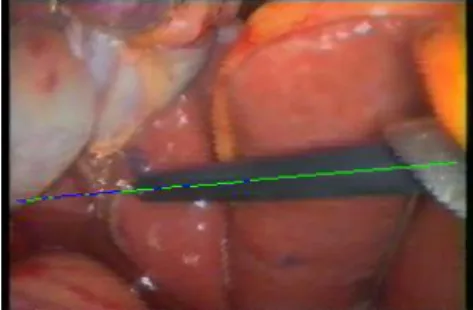
We were able to perform the tracking of an instrument when the specular re-flections were limited. The computation time is around 100 ms for a 200x100 image. It allows for smooth tracking when the instrument is moved at a usual speed. The computation time could still be reduced by optimizing the code, al-lowing us to take into account abrupt and large movements. As we said earlier, a resolution of 200x100 pixels is enough for the tracking of a laparoscopic in-strument, since we are not looking for subpixel precision to control the camera. We considered that the tool was centered as long as the distance between the detected tip and the previous tip was less than 11 pixels. Fig. 25 shows the distance in pixels between the tip found by the method and the tip manually selected. In 70% of the images, the error is inferior to 5 pixels, and in 87 % the error is less than 11 pixels.
Figure 25: Error in pixels between the tip found by the method and the tip selected manually and an example of correct detection (yellow dots: candidate points, red points: points corresponding to the axis, blue dot on the axis: tip of the instrument).
4.2.3 Error analysis
We analyzed the images which gave important errors in order to understand the reasons that could cause the method to fail. Fig. 26 shows some examples of false detection in the sequence.
a) b) c)
Figure 26: a) Wrong detection due to a lack of contrast, b) wrong detection due to specular reflections, c) wrong detection of the axis.
Fig. 26 a) corresponds to the first error peak (frame 9). The detection of the axis is correct, but the tip is wrongly positioned. The red segments correspond to the pixels labelled as pixels belonging to the instrument, and the yellow segments as pixels labelled as the background. Since the background in the area of the tip is very dark, it is wrongly labelled by the Otsu threshold as a region belonging to the instrument. This is also the cause of the error for frames 35, 36, 61, 63 and 64.
Fig 26 b) corresponds to the second error peak (frame 21). Again, the axis is correctly detected, but not the tip. This time, the error is due to specular reflections, which are labelled as background. This also causes errors for frames 67 and 69. The important error for frame 37 is caused by a false detection of the axis of the tool (Fig. 26 c): the edges of the instrument are barely visible in the image because of the lack of contrast, and the organ on the far hand side of the
if we replace frame 37 with an image of better resolution (410x410 pixels), the axis is detected correctly (27).
a) b)
Figure 27: The detection of the instrument axis, which failed for frame 37 with a resolution of 200x100 pixels (see Fig. 26 c) ) is successful with a resolution of 410x410 pixels: a) original image, b) result of the detection.
While the specular reflecions are important, they do not deteriorate the detection of the axis, since they are along the axis of the instrument. However, they cause failure in tip detection, because the wrong classes are attributed to the instrument and background.
5
Discussion
In this paper, we proposed a new method for the tracking of instruments in laparoscopic surgery, based on the measurement of the position of their insertion points in the abdominal cavity. It is based on the assumption that the insertion points are relatively fixed during the surgical procedure. We validated this assumption by measuring the position of an insertion point through time during a cadaver experiment. During a real intervention with a living patient, the movement of the abdominal wall caused by breathing can be considered as null or very limited, since the abdominal cavity is insuflated with gas. The movements of the instruments could cause the insertion point to move slightly, but these potential movements are partly considered by increasing the radius of the circle C (section 3.2).
This experiment also allowed us to test our approach in conditions that are close to a real intervention. We were able to perform the tracking of an instrument when it is moved at a usual speed and when the specular reflections are limited. The speed of the method could be improved by optimization of the code and by using a region of interest (ROI) around the tip detected in the previous image. However, this ROI must be carefully selected because of the important magnification of an endoscope, and because the instrument can have large and quick movements (for instance when the surgeon is cutting tissues).
We were also able to identify the reasons that could cause the failure of the detection. One of the most important problems to solve is the problem of specular reflections, which is mostly problematic for the detection of the tip of the instrument. A first lead could be to work in a color space less sensitive to specular reflections such as HSI. Gr¨oger et al. have addressed the problem of specular reflection removal on images of the heart surface in [27], but the real-time constraint is hard to meet. Since the detection of the axis is quite robust
to specular reflections, we could perhaps only remove the specular reflections in a ROI around the instrument. A simple solution to detect the specular reflections would be to analyse an image of a white object at the beginning of the intervention. This could be easily integrated into the surgical procedure, since the surgeon performs this step to tune the light source.
Although very quick, the Otsu threshold might not be the best classification method to separate the points corresponding to the instrument from the points corresponding to the background. Two pixels with a different color but the same color level are treated identically, and since the Otsu threshold separates the points in only two classes, the classification might fail if there are a lot of specular reflections or if the contrast varies too much in the background. We should investigate more complex segmentation algorithms dedicated to color images to improve this step.
In the images where several instruments were visible, we explained that we could have difficulties in determining the position of the tip. However, the detection of the tip might not be necessary. The intersection points of the symmetry axis of the instruments roughly indicate the area of interest in the image.
It must also be noted that if the portion of the instrument in the image is too small, the amount of points obtained at the segmentation phase is not sufficient to detect the axis. Also, if the instrument is only partly in the image (one edge is not visible), the axis cannot be found. If the instrument is very close to the camera, or the zoom factor is very high, only the tip of the instrument is visible, and for some instruments such as pliers, our shape model (section 3.2) might not be accurate, but we will consider defining more complex shape models in the future.
Finally, we must avoid false detections as much as possible. Our method deals with them in part; If the amount of edge points which voted for the axis is too low, or if the length of the instrument is too small, an error is raised. If the tool was correctly detected in the first image, its color and the background color are stored for the next images. Thus, if the detection algorithm finds a tool with a color very close to the color of the background, an error is raised. If an error is raised although an instrument was visible in the image (false nega-tive), the robot doesn’t move and the next image is processed. However, if the method finds a tip although no instrument is visible in the image (false posi-tive), the robot will move towards an undesired position. Although the surgeon can interrupt the tracking at any time with the dead man switch (see section 2), these unwanted movements must occur as rarely as possible. One solution to address this problem could be to gather a few images of the abdominal cavity without an instrument at the beginning of the intervention in order to obtain information about the color of the background.
6
Conclusion - Future work
We developed a novel method to detect an instrument in laparoscopic images. This method is automatic, almost real-time, and robust to artefacts such as smoke or small partial occlusion. Our first cadaver test allowed us to validate our approach, especially concerning the approach of using the insertion points of the instruments, and allowed us to gain some insight on the principal difficulties
we still need to solve. We plan on using this method to develop and compare different tracking strategies (see Fig. 1). The exploitation of the insertion points has a potential interest for more complex systems than a camera holder. Acknowledgements: This project was partially funded by the French Ministry of Research and Technology under a CIT (Center for Innovation and Technol-ogy) grant.
The authors would like to thank Bruno Thibaut from the anatomy laboratory of the Medical University of Grenoble for his help during our experiments.
References
[1] B. Makhoul, A. De La Taille, D. Vordos, L. Salomon, P. Sebe et al., La-paroscopic radical nephrectomy for T1 renal cancer: the gold standard? A comparison of laparoscopic vs open nephrectomy. BJU International 2004, Vol. 93, pp. 67-70, 2004.
[2] P. Ballester, Y. Jain, K. R. Haylett and R. F. McCloy: Comparison of task performance of robotic camera holders EndoAssist and Aesop. International Congress Series, Vol. 1230, pp. 1100-1103, June 2001.
[3] L. R. Kavoussi, R. G. Moore, J. B. Adams et al., Comparison of robotic versus human laparoscopic camera control, J Urol, 154:2134, 1995
[4] P. A. Finlay, Clinical Experience With a Goniometric Head-Controlled La-paroscope Manipulator. www.amstrong-healthcare.com/
[5] A. Nishikawa, T. Hosoi, K. Koara, D. Negoro, A. Hikita et al., Real-Time Visual Tracking of the Surgeon’s Face for Laparoscopic Surgery. MICCAI 2001, Vol. 2208, pp. 9-16, 2001.
[6] P. Ballester, Y. Jain, K.R. Haylett, and R.F. McCloy, Comparison of task performance of robotic camera holders EndoAssist and AESOP. proc. of the 15th Intl. congress and exhibition of Computer Assisted Radiology and Surgery, Elsevier science, p. 1071-1074, 2001.
[7] V.F. Munoz, I. Garcia-Morales, C. Perez del Pulgar, J.M. Gomez-DeGabriel, J. Fernandez-Lozano et al., Control movement scheme based on manipu-lability concept for a surgical robotic assistant. Proceedings of the IEEE International Conference on Robotics and Automation, 2006.
[8] S.-Y. Ko, J. Kim, D.S. Kwon, and W.-J. Lee, Intelligent Interaction be-tween Surgeon and Laparoscopic Assistant Robot System. IEEE Interna-tional Workshop on Robots and Human Interactive Communication, pp. 60-65, 2005.
[9] O. Tonet, T.U. Ramesh, G. Megali, P. Dario, Image analysis-based approach for localization of endoscopic tools. Proceedings of Surgetica’05, pp. 221-228, 2005.
[10] A. Krupa, J. Gangloff, C. Doignon, M. de Mathelin, G. Morel et al., Au-tonomous 3-D positioning of surgical instruments in robotic laparoscopic surgery using visual servoing. IEEE Trans. on Robotics and Automation, vol. 19(5), pp. 842-53, 2003.
[11] G. Wei, K. Arbter, G. Hirzinger, Real-Time Visual Servoing for Laparo-scopic Surgery. Controlling Robot Motion with Color Image Segmentation. IEEE Eng. in Med. and Biol., pp. 40-45, 1997.
[12] A. Casals, J. Amat and E. Laporte, Automatic Guidance of an Assistant Robot in Laparoscopic Surgery. Proceedings of the IEEE International Con-ference on Robotics and Automation, pp. 895-900, 1996.
[13] Yuang Wang, D. R. Uecker and Yulun Wang, A new framework for vision enabled and robotically assisted minimally invasive surgery. Computerized Med. Imaging and Graphics, Vol. 22, pp. 429-37, 1998.
[14] C. Doignon, F. Nageotte and M. de Mathelin, Detection of grey regions in color images: application to segmentation of a surgical instrument in robo-tized laparoscopy. Proceedings of 2004 IEEE/RSJ International Conference on Intelligent Robots and Systems, pp. 3394-3399, 2004.
[15] J. Climent and P. Mars, Automatic instrument localization in laparoscopic surgery. Electronic Letters on Computer Vision and Image Analysis, 4(1), pp. 21-31, 2004.
[16] D. Burschka, J. Corso, M. Dewan, W. Lau, M. Li et al., Navigating In-ner Space: 3-D Assistance for Minimally Invasive Surgery, Robotics and Autonomous Systems, 52(1), pp. 5-26, 2005.
[17] www.intuitivesurgical.com
[18] P. J. Berkelman, Ph. Cinquin, J. Troccaz, J-M. Ayoubi, C. L´etoublon, Development of a Compact Cable-Driven Laparoscopic Endoscope Manipu-lator. MICCAI 2002, Vol. 2488, pp. 17-24, 2002.
[19] E. Malis, F.Chaumette and S. Boudet, 2-1/2-D Visual Servoing, IEEE Transactions on Robotics and Automation, Vol. 15, NO. 2, pp. 238-250, April 1999.
[20] http://www.intel.com/technology/computing/opencv/index.htm
[21] Z. Zhang, A Flexible New Technique for Camera Calibration. IEEE Trans. on PAMI, 22(11) pp. 1330-34, 2000.
[22] C. Doignon, F. Nageotte and M. de Mathelin, Segmentation and Guidance of Multiple Rigid Objects for Intra-Operative Endoscopic Vision. Proceed-ings of the Workshop on Dynamical Vision of ECCV 2006.
[23] O. Faugeras, Three Dimensional Computer Vision. A Geometric Viewpoint. The MIT press, 1993.
[25] Richard O. Duda and Peter E. Hart, Use of the Hough Transformation To Detect Lines and Curves in Pictures. Communications of the ACM, Vol. 15(1), pp. 11-15, 1972.
[26] N. Otsu, A threshold selection method from gray level histograms. IEEE Trans. Systems, Man and Cybernetics, Vol. 9, pp. 62-66, 1979.
[27] M. Gr¨oger, W. Sepp, T. Ortmaier and G. Hirzinger, Reconstruction of Image Structure in Presence of Specular Reflections, DAGM 2001, LNCS 2191, pp. 5360, 2001.