HAL Id: hal-01243700
https://hal.inria.fr/hal-01243700
Submitted on 27 May 2016
HAL is a multi-disciplinary open access
archive for the deposit and dissemination of
sci-entific research documents, whether they are
pub-lished or not. The documents may come from
teaching and research institutions in France or
abroad, or from public or private research centers.
L’archive ouverte pluridisciplinaire HAL, est
destinée au dépôt et à la diffusion de documents
scientifiques de niveau recherche, publiés ou non,
émanant des établissements d’enseignement et de
recherche français ou étrangers, des laboratoires
publics ou privés.
Disassembling Low-level Self-modifying Code
Sandrine Blazy, Vincent Laporte, David Pichardie
To cite this version:
Sandrine Blazy, Vincent Laporte, David Pichardie. Verified Abstract Interpretation Techniques for
Disassembling Low-level Self-modifying Code. Journal of Automated Reasoning, Springer Verlag,
2016, 56 (3), pp.26. �10.1007/s10817-015-9359-8�. �hal-01243700�
Verified Abstract Interpretation Techniques for
Disassembling Low-level Self-modifying Code
Sandrine Blazy ¨ Vincent Laporte ¨ David Pichardie
Received: date / Accepted: date
Abstract Static analysis of binary code is challenging for several reasons. In particular, standard static analysis techniques operate over control-flow graphs, which are not available when dealing with self-modifying programs which can modify their own code at runtime. We formalize in the Coq proof assistant some key abstract interpretation techniques that automatically extract memory safety properties from binary code. Our analyzer is formally proved correct and has been run on several self-modifying challenges, provided by Cai et al. in their PLDI 2007 article.
Keywords Coq ¨ abstract interpretation ¨ low-level programming language Publication history: this article is a revised and extended version of the paper “Verified Abstract Interpretation Techniques for Disassembling Low-level Self-modifying Code” published in the ITP 2014 conference proceedings.
1 Introduction
Abstract interpretation [16] provides advanced static analysis techniques with strong semantic foundations. It has been applied on a large variety of program-ming languages. Still, specific care is required when adapting these techniques
This work was supported by Agence Nationale de la Recherche, grant number ANR-11-INSE-003 Verasco.
S.Blazy
Université Rennes 1 – IRISA – Inria, Campus de Beaulieu, Rennes, France E-mail: [email protected]
V.Laporte
Université Rennes 1 – IRISA – Inria, Campus de Beaulieu, Rennes, France E-mail: [email protected]
D.Pichardie
ENS Rennes – IRISA – Inria, Campus de Beaulieu, Rennes, France E-mail: [email protected]
to low-level code, specially when the program to be analyzed comes in the form of a sequence of bits and must first be disassembled. Disassembling is the process of translating a program from a machine friendly binary format to a textual representation of its instructions. It requires to decode the instructions (i.e., understand which instruction is represented by each particular bit pattern) but also to precisely locate the instructions in memory. Indeed instructions may be interleaved with data or arbitrary padding. Moreover once encoded, instructions may have various byte sizes and may not be well aligned in memory, so that a single byte may belong to several instructions.
To thwart the problem of locating the instructions in a program, one must follow its control-flow. However, this task is not easy because of the indirect jumps, whose targets are unknown until runtime. A static analysis needs to predict with enough precision, given an expression denoting a jump target, the values it may evaluate to.
In addition, instructions may be produced at runtime, as a result of the very execution of the program. A simple example is the modification of some operands (e.g., registers) of existing instructions. Another example is the creation of new sequences of instructions in existing code. Such programs are called self-modifying programs; they are commonly used in security as an obfuscation technique (e.g., to protect the intellectual property of the program authors, to increase the stealth of malware) [33], as well as in just-in-time compilation and in operating systems (mainly for improving performances).
Analyzing a binary code is mandatory when this code is the only available part of a software. Because the instructions of a self-modifying program are not the instructions that will be executed, most of standard reverse engineering tools (e.g., the IDA Pro disassembler and debugger, a de facto standard for the analysis of binary code) cannot disassemble and analyze self-modifying programs. In order to disassemble and analyze such programs, one must very precisely understand which instructions are written and where. And for all programs, one must check every single memory write to decide whether it modifies the program code.
As the real code of a self-modifying program is hidden and varies over time, self-modifying programs are also beyond the scope of the vast majority of formal semantics of programming languages. Indeed a prerequisite in such semantics is the isolation and the non-modification of code in memory. Turning to verified static analyses, they operate over toy languages [8, 27] or more recently over realistic C-like languages [32, 6], but they assume that the control-flow graph is extracted by a preliminary step, and thus they do not encompass techniques devoted to self-modifying code.
In this paper, we formalize with the Coq proof assistant key static analysis techniques to predict the possible targets of the computed jumps and make precise which instructions alter the code and how, while ensuring that the other instructions do not modify the program. Our static analysis techniques rely on two main components classically used in abstract interpretation, abstract domains and fixpoint iterators, that we detail in this paper.
Our formalization effort is divided in three parts. Firstly, we formalize a small binary language in which code is handled as regular mutable data. Secondly, we formalize and prove correct an abstract interpreter that takes as input an initial memory state, computes an over-approximation of the reachable states that may be generated during the program execution, and then checks that all reachable states maintain memory safety. Finally, we extract from our formalization an executable OCaml tool that we run on several self-modifying challenges, provided by Cai et al. [11].
The article makes the following contributions.
– We push further the limit in terms of verified static analysis by tackling the specific challenge of binary self-modifying programs, such as fixpoint iteration without control-flow graph and simple trace partitioning [22]. – We provide a complementary approach to [11] by automatically inferring the
required state invariants that enforce memory safety. Indeed, the axiomatic semantics of [11] requires programs to be manually annotated with invariants written in a specific program logic.
The remainder of this article is organized as follows. First, Section 2 briefly introduces the static analysis techniques we formalized. Then, Section 3 defines the semantics of our low-level language. Section 4 details our abstract interpreter. Section 5 describes some improvements that we made to the abstract interpreter, as well as the experimental evaluation of our implementation. We finish this article by a discussion of related work in section Section 6, followed by future work and conclusions in section Section 7.
Availability The Coq development underlying this article can be consulted
on-line at http://www.irisa.fr/celtique/ext/smc.
Notations Option types are used to represent potential failures. For functions
returning “option” types, txu (read: “some x”) corresponds to success with return value x, and H (read: “none”) corresponds to failure. In the context of abstract interpretation, where abstract values represent sets of concrete values, it is often convenient to distinguish two interpretations of such an option type: the absence of a definite value may be interpreted as the empty set or as the full set. Therefore, we introduce two different option types,botlift Aandtoplift A, abbreviated respectivelyA+KandA+J:
Inductive botlift (A:Type) : Type := Bot | NotBot (x:A). Inductive toplift (A:Type) : Type := All | Just (x:A).
Notation "A +K" := (botlift A). Notation "A +J" := (toplift A).
These types are equipped with a monad structure; hence we use standard operators bind, lift and notation do a Ð m; b. We note K forBot, J for Top, and overload the notation txu forNotBot xandJust x.
2 Disassembling by Abstract Interpretation
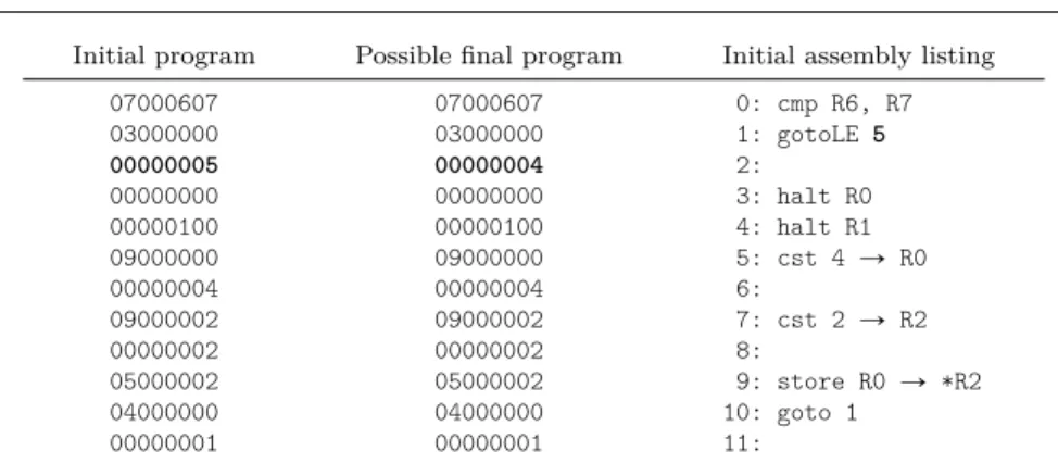
We now present the main principles of our analysis on the program shown in Figure 1. It is printed as a sequence of bytes (on the extreme left) as well
Initial program Possible final program Initial assembly listing 07000607 07000607 0: cmp R6, R7 03000000 03000000 1: gotoLE 5 00000005 00000004 2: 00000000 00000000 3: halt R0 00000100 00000100 4: halt R1 09000000 09000000 5: cst 4 Ñ R0 00000004 00000004 6: 09000002 09000002 7: cst 2 Ñ R2 00000002 00000002 8: 05000002 05000002 9: store R0 Ñ *R2 04000000 04000000 10: goto 1 00000001 00000001 11:
Figure 1 A self-modifying program: as a byte sequence (left); after some execution steps (middle); assembly source (right).
as under a disassembled form (on the extreme right) for readability purposes. This program, as we will see, is self-modifying, so these bytes correspond to the initial content of the memory from addresses 0 to 11. The remainder of the memory (addresses in r´231; ´1s Y r12; 231
´ 1s), as well as the content of the registers, is unknown and can be regarded as the program input.
All our example programs target a machine operating over a low-level memory made of 232 cells, eight registers, and flags — boolean registers that
are set by comparison instructions. Each memory cell or register stores a 32 bits integer value, that may be used as an address in the memory. Programs are stored as regular data in the memory; their execution starts from address zero.
Nevertheless, throughout this paper we write the programs using the follow-ing custom syntax. The instructioncst v Ñ rloads registerrwith the given valuev. The instruction cmp r, r’ denotes the comparison of the contents of registersrandr’. The instructiongotoLE dis a conditional jump tod, it is taken if in the previous comparison the content ofr’was less than or equal to the one of r;goto dis an unconditional jump tod. The instructionsload *r Ñ r’
andstore r’ Ñ *rdenote accesses to memory at the address given in registerr; andhalt rhalts the machine with as final value the content of registerr.
The programming language we consider is inspired from x86 assembly; notably instructions have variable size (one or two bytes, e.g., the length of the instructiongotoLE 5stored at line 1 is two bytes, the byte03000000forgoto and one byte for5) and conditional jumps rely on flags. In this setting, a program is no more than an initial memory state, and a program point is simply the address of the next instruction to execute.
In order to understand the behavior of this program, one can follow its code as it is executed starting from the entry point (byte 0). The first instruction
cmp R6, R7 compares the (statically unknown) content of two registers. This comparison modifies only the states of the flags. Then, thegotoLE 5instruction is executed and, depending on the outcome of this comparison, the execution proceeds either to the following instruction (stored at byte 3), or from byte 5.
Since the analysis cannot predict which branch will be taken, both branches must be analyzed.
Executing the block from byte 5 will modify the byte 2 belonging to the
gotoLEinstruction (highlighted in Figure 1); more precisely it will change the jump destination from 5 to 4: thestore R0 Ñ *R2instruction writes the content of registerR0(namely 4) in memory at the address given in registerR2(namely 2). Notice that a program may directly read from or write to any memory cell: we assume that there is no protection mechanism as provided by usual operating systems. After the modification is performed, the execution jumps back to the modified instruction, jumps to byte 4 then halts, with final value the content of registerR1.
This example highlights that the code of a program (or its control-flow graph) is not necessarily a static property of this program: it may vary as the program runs. To correctly analyze such a program, one must discover, during the fixpoint iteration, the two possible states of the goto instruction at program points 1 and 2 and its two possible targets (i.e., 4 and 5). More specially, we need at least to know, for each program point (i.e., memory location), which instructions may be decoded from there when the execution reaches this point. This in turn requires to know what are the values that the program operates on. We therefore devise a value analysis that computes, for each reachable program point (i.e., in a flow sensitive way) an over-approximation of the content of the memory and the registers, and the state of the flags, when the execution reaches that point.
The analysis relies on a numeric abstract domain N7 that provides a
rep-resentation for sets of machine integers and abstract arithmetic operations.
γNP N7Ñ Ppintq denotes the associated concretization function. Relying on
such a numeric domain, one can build abstract transformers. They model the execution of each instruction over an abstract memory that maps locations (i.e., memory addresses1and registers) to abstract numeric values. An abstract state
is then a mapping that attaches such an abstract memory to each program point of the program, and thus belongs toaddrÑ`paddr`regq Ñ N7˘.
To perform one abstract execution step, from a program point pp and an abstract memory state m7 that is attached to pp, we first enumerate all
instructions that may be decoded from the set γNpm7pppqq. Then for each of
such instructions, we apply the matching abstract transformer. This yields a new set of successor states whose program points are dynamically discovered during the fixpoint iteration.
The abstract interpretation of a whole program iteratively builds an approx-imation executing all reachable instructions until nothing new is learned. This iterative process may not terminate, since there might be infinite increasing chains in the abstract search space. As usual in abstract interpretation, we accel-erate the iteration using widening operations [16]. Once a stable approximation is finally reached, an approximation of the program listing or control-flow graph can be produced.
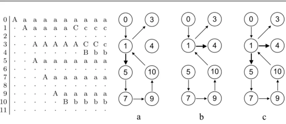
0 A a a a a a a a a a 1 ¨ A a a a a C c c c 2 ¨ ¨ ¨ ¨ ¨ ¨ ¨ ¨ ¨ ¨ 3 ¨ ¨ A A A A A C C c 4 ¨ ¨ ¨ ¨ ¨ ¨ ¨ B b b 5 ¨ ¨ A a a a a a a a 6 ¨ ¨ ¨ ¨ ¨ ¨ ¨ ¨ ¨ ¨ 7 ¨ ¨ ¨ A a a a a a a 8 ¨ ¨ ¨ ¨ ¨ ¨ ¨ ¨ ¨ ¨ 9 ¨ ¨ ¨ ¨ A a a a a a 10 ¨ ¨ ¨ ¨ ¨ B b b b b 11 ¨ ¨ ¨ ¨ ¨ ¨ ¨ ¨ ¨ ¨ 4 1 0 3 5 7 9 10 4 1 0 3 5 7 9 10 4 1 0 3 5 7 9 10 a b c
Figure 2 Iterative fixpoint computation
To illustrate this process, Figure 2 shows how the analysis of the program from Figure 1 proceeds. We do not expose a whole abstract memory but only the underlying control-flow graph it represents. On this specific example, three different graphs are encountered during the analysis. For each program pointpp, we represent a node with same name and link it with all the possible successor nodes according to the decoding of the set γNpm7pppqq. The array shows the
construction of the fixpoint: each line represents a program point and the columns represent the iterations of the analysis. In each array cell lies the name of the control-flow graph representing the abstract memory for the given program point during the given iteration; a dot stands for an unreachable program point. The array cells whose content is in upper case highlight the program points that need to be analyzed: they are the worklist.
Initially, at iteration 0, only program point 0 is known to be reachable and the memory is known to exactly contain the program denoted by the first control-flow graph (called a in Figure 2 and corresponding to the initial program of Figure 1). The only successor of point 0 is point 1 and it is updated at the next iteration. After a few iterations, point 9 is reached and the abstract control-flow graph a is updated into the control-flow graph b that is propagated to point 10. This control-flow graph corresponds to the possible final program of Figure 1, where program-point 5 became unreachable. At the next iteration, program point 1 (i.e., the loop condition) is reached again and the control-flow graph b is updated into the control-flow graph c that correspond to the union of the two previous control-flow graphs. After a few more iterations, the process converges.
In addition to a control-flow graph or an assembly listing, more properties can be deduced from the analysis result. We can prove safety properties about the analyzed program, like the fact that its execution is never stuck.
The analysis produces an over-approximation of the set of reachable states. In particular, a superset of the reachable program points is computed, and for each of these program points, an over-approximation of the memory state when the execution reaches this program point is available. Thus we can check that for every program point that may be reached, the next execution step
Definition addr := Int.int.
Inductive reg := R0 | R1 | R2 | R3 | R4 | R5 | R6 | R7. Inductive flag := FLE | FLT | FEQ.
Inductive comparison := Ceq | Cne | Clt | Cle | Cgt | Cge.
Inductive binop := OpAdd | OpSub | OpMul | OpDivs | OpShl | OpShr | OpShru | OpAnd | OpOr | OpXor | OpCmp (c: comparison) | OpCmpu (c: comparison). Inductive instruction :=
(* arithmetic *)
| ICst (v:int) (dst:reg) | ICmp (src dst: reg) | IBinop (op: binop) (src dst: reg)
(* memory *)
| ILoad (src dst: reg) | IStore (src dst: reg)
(* control *)
| IGoto (tgt: addr) | IGotoInd (r: reg) | IGotoCond (f: flag) (tgt: addr) | ISkip | IHalt (r: reg).
Figure 3 Abstract syntax of our low-level language
from this point cannot be stuck. This verification procedure is formally verified, as described in the following section.
3 Semantics of our Binary Language
This section defines the abstract syntax and semantics of the low-level language our static analyzer operates over. The semantics uses a decoding function from binary code to our low-level language. The semantics is presented as a small-step operational semantics that can observe self-modifying programs.
3.1 Abstract Syntax
The programming language in which are written the programs to analyze is formalized using the abstract syntax shown on Figure 3. In the Coq formaliza-tion, the abstract syntax is presented as inductive data types. Machine integers (typeint) are those of the CompCert libraryIntof 32 bits machine integers [5]. The eight registers of our language are called R0, . . . R7and there are three register flags calledFLE(for “less or equal” comparisons),FLT(for “less than” comparisons) andFEQ(for “equality” comparisons).
Instructions are either arithmetic expressions, or memory accesses or control-flow instructions. Instructions for accessing memory areILoad andIStore; their operands are registers. So as to keep the language simple, memory accesses are limited to these two instructions: the other instructions, which are described next, only operate on registers. Arithmetic expressions consist of integer con-stants, signed comparisons and binary operations. Control-flow instructions consist of unconditional and conditional jump instructions, the empty instruc-tion ISkip and the IHaltinstruction which halts the program execution. For
unconditional jumps, we distinguish register-indirect jumps (IGotoInd r instruc-tions, whereris a register) from other jumps (i.e., absolute jumps, written as
IGoto v, wherev is a literal constant address).
In a binary language, there is no distinction between code and data: a value stored in memory can be interpreted either as representing data or as encoding instructions. So as to model a binary language, we first introduce a decoding function calleddec. Its type is(addr→int) → pp → option(instructionˆnat). Given a memorymemof typeaddr → int(i.e., a function from addresses to values) and an addressppof typeaddr, this function yields the instruction stored at this address along with its byte size (so as to know where the next instruction begins). This size is of typenat, the Coq type for natural numbers. Since not all integer sequences are valid encodings, this decoding may fail (hence the
optiontype). In order to be able to conveniently write programs, there is also a matching encoding function calledenc, whose type isinstruction → list int. However the development does not depend on it at all: properties are stated in terms of already encoded programs.
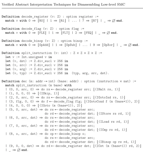
The decoding function is defined in Figure 4. The binary decoding of a sequence of bytes stored in memorymat program pointppis written(dec m pp). A successful decoding yields a pair(i,sz), whereszis the size ofi, the instruction stored at addressppin m2.
The binary format of instructions is arbitrary and has little impact on the design of the analyzer. We rely on the fact that the encoding length can be inferred from the first byte of any encoded instruction3. The self-modifying
programs that we consider rely on the particular encoding that we chose. This encoding works as follows. Instructions that hold a value (e.g.,IGoto 5) require two bytes: the value occupies the second byte; other instructions require one byte. The first byte is made of four fields of one octet each: the decoding of this first byte first extracts the content of each field using Euclidean divisions (performed by thesplit_instructionfunction). The first field (typ) corresponds to the constructor of theinstructiondata type. From its value, one can deduce the size of the instruction and how to interpret the next fields. The second field (flg) holds a flag (only used in theIGotoCondinstruction). The third and fourth fields hold respectively the source and destination registers. Depending on the instruction, none, both or only one of them may be relevant. Unused fields always have the value zero. This encoding is very sparse: many byte sequences do not represent any valid instruction. Moreover, in the decoding function, errors are propagated by the bind operator of the error monad, written
do a ← m; b.
2 The size cannot be deduced from the instruction as: 1. the encoding function is not
known; and 2. they may be several encodings, of various sizes, for a single instruction.
3 This is not the case, for instance, of the encoding of x86 instructions, that may begin
Definition decode_register (v: Z) : option register :=
match v with 0 ñ tR0u | 1 ñ tR1u | ... | 7 ñ tR7u | _ ñ H end. Definition decode_flag (v: Z) : option flag :=
match v with 0 ñ tFLEu | 1 ñ tFLTu | 2 ñ tFEQu | _ ñ H end. Definition decode_binop (v: Z) : option binop :=
match v with 0 ñ tOpAddu | 1 ñ tOpSubu | ... | 9 ñ tOpXoru | _ ñ H end. Definition split_instruction (v: int) : Z ˆ Z ˆ Z ˆ Z :=
let v := Int.unsigned v in
let (v, dst) := Z.div_eucl v 256 in let (v, src) := Z.div_eucl v 256 in let (v, arg) := Z.div_eucl v 256 in
let (v, typ) := Z.div_eucl v 256 in (typ, arg, src, dst).
Definition dec (m: addr Ñ int) (base: addr) : option (instruction ˆ nat) := match split_instruction (m base) with
| (0, 0, src, 0) ñ do rs Ð decode_register src; t(IHalt rs, 1)u | (1, 0, 0, 0) ñ t(ISkip, 1)u
| (2, 0, src, 0) ñ do rs Ð decode_register src; t(IGotoInd rs, 1)u | (3, flg, 0, 0) ñ do f Ð decode_flag flg; t(IGotoCond f (m (base+1)), 2)u | (4, 0, 0, 0) ñ t(IGoto (m (base+1)), 2)u
| (5, 0, src, dst) ñ do rs Ð decode_register src;
do rd Ð decode_register dst; t(IStore rs rd, 1)u | (6, 0, src, dst) ñ do rs Ð decode_register src;
do rd Ð decode_register dst; t(ILoad rs rd, 1)u | (7, 0, src, dst) ñ do rs Ð decode_register src;
do rd Ð decode_register dst; t(ICmp rs rd, 1)u | (8, o, src, dst) ñ do op Ð decode_binop o;
do rs Ð decode_register src;
do rd Ð decode_register dst; t(IBinop op rs rd, 1)u | (9, 0, 0, dst) ñ do rd Ð decode_register dst; t(ICst (m (base+1)) rd, 2)u | _ ñ H end.
Figure 4 Decoding binary code
3.2 Semantics
The language semantics is given as a small-step transition relation between machine states. A machine state may be xpp, f, r, my whereppis the current
program point (address of the next instruction to be executed),fis the current flag state,ris the current register state, and m is the current memory. Such a tuple is called a machine configuration (typemachine_config). Otherwise, a machine state is rvs, meaning that the program stopped returning the valuev.
Values are machine integers (typeint).
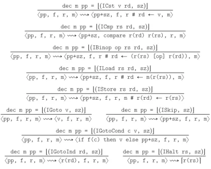
The semantics is defined in Figure 5 as a set of rules of the following shape:
dec m pp = tpi, szqu
xpp, f, r, my ù xpp’, f’, r’, m’y.
The premise states that decoding the bytes in memorymfrom address pp
Definition compare (i j: int) (f: flag) : bool := match f with
| FLE ñ negb (Int.lt j i) | FLT ñ Int.lt i j | FEQ ñ Int.eq i j end. dec m pp = tpICst v rd, szqu
xpp, f, r, my ù xpp+sz, f, r # rd Ð v, my dec m pp = tpICmp rs rd, szqu
xpp, f, r, my ù xpp+sz, compare r(rd) r(rs), r, my dec m pp = tpIBinop op rs rd, szqu
xpp, f, r, my ù xpp+sz, f, r # rd Ð (r(rs) [op] r(rd)), my dec m pp = tpILoad rs rd, szqu
xpp, f, r, my ù xpp+sz, f, r # rd Ð m(r(rs)), my dec m pp = tpIStore rs rd, szqu
xpp, f, r, my ù xpp+sz, f, r, m # r(rd) Ð r(rs)y dec m pp = tpIGoto v, szqu
xpp, f, r, my ù xv, f, r, my
dec m pp = tpISkip, szqu xpp, f, r, my ù xpp+sz, f, r, my dec m pp = tpIGotoCond c v, szqu
xpp, f, r, my ù xif f(c) then v else pp+sz, f, r, my dec m pp = tpIGotoInd rd, szqu
xpp, f, r, my ù xr(rd), f, r, my
dec m pp = tpIHalt rs, szqu xpp, f, r, my ù rr(rs)s Figure 5 Concrete semantics
how to execute a particular instruction at program point pp in memory m
with flag state f and register stater. In each case, most of the state is kept unchanged. Instructions that are not branching proceed their execution at program pointpp+sz(sinceszis the size of this instruction once encoded). In the rules, the notations # id Ð v stands for the update of stateswith a new valuevof register or memory cellid.
InstructionICst v rdupdates destination registerrdwith valuev. Instruction
ICmp rs rdupdates the flag state according to the comparison (compare) of the values held by the two involved registers. InstructionIBinop op rs rdapplies the denotation[op]of the given binary operatoropto the contentsr(rs) and
r(rd)of registersrsandrd. Then, it updates the state of register rd: inr, the new value ofrdthus becomesr(rs) [op] r(rd). InstructionILoad rs rdupdates register rdwith the value m(r(rs)) found in memory at the address given in registerrs. Instruction IStore rs rdupdates the memory at the address given in registerrdwith the value given in registerrs.
InstructionIGoto vsets the program point tov. InstructionISkip does noth-ing: execution proceeds at next program point. Conditional jump instruction
IGotoCond c vjumps to address v or falls through to pp+sz depending on the current state of flagc. Indirect jump instructionIGotoInd rdproceeds at the
pro-gram point found in registerrd. InstructionIHalt rsterminates the execution, returning the content of registerrs.
Finally, we define the semantics vPw of a programPas the set of states s that are reachable from an initial state x0, f, r, Py, with current program point zero and memoryP (where ù‹ denotes the reflexive-transitive closure of the
small-step relation):
vPw “ ts | Df r, x0, f, r, Py ù‹su .
Notice that the program Pbelongs to the state: it is initially known, but can be modified as the execution goes on.
4 Abstract Interpreter
The static analyzer is specified, programmed and proved correct using the Coq proof assistant. This involves several steps that are described in this section: designing abstract domains and abstract semantics, as well as writing a fixpoint iterator, and lastly stating and proving soundness properties about the results of the static analysis.
In order to analyze programs, we build an abstract interpreter, i.e., an executable semantics that operates over abstract elements, each of them rep-resenting many concrete machine configurations. Such an abstract domain provides operators that model basic concrete operations: read a value from a register, store some value at some address in memory, and so on. The static analyzer then computes a fixpoint within the abstract domain, that over-approximates all reachable states of the analyzed program. We first describe our abstract domain before we head to the abstract semantics and fixpoint computation.
4.1 Abstract Domains
Our abstract interpreter operates over an abstract memory domain. This abstract domain handles a (simplified) lattice structure, plus some abstract transformers that we describe below. It is parameterized by a numeric abstract domain that abstracts numerical values. The same notion of lattice structure is used in both signatures. We now describe these different signatures.
Weak Lattice. Each abstract domain handles a set of lattice operators that
are convenient for programming abstract transformers and performing fixpoint computation. Figure 6 presents the type classweak_lattice. It is parameterized by a carrier typeAand handles an order testleb, a top element, a join operator and a widening operator. The class only contains the operator signatures and not their specifications.
Class weak_lattice (A: Type) : Type := { leb: A Ñ A Ñ bool; top: A; join: A Ñ A Ñ A; widen: A Ñ A Ñ A }.
Class gamma_op (A B: Type) : Type := γ : A Ñ P (B).
Record adom (A B:Type) (WL: weak_lattice A) (Gamma: gamma_op A B) : Prop := { gamma_monotone: @ a1 a2, leb a1 a2 = true Ñ γ a1 Ď γ a2;
gamma_top: @ x, x P γ top;
join_sound: @ x y, γ x Y γ y Ď γ (join x y) }.
Figure 6 Signature of weak lattices and concretizations
In the same figure, we provide the record signature adom that contains soundness specifications forleb,topandjoin. We rely on an abstract interpre-tation methodology that only manipulates concretization functions, instead of full Galois connections (see [9] for a discussion about this design choice). The concretization operator γ transforms an abstract element into its counter-part concrete property (i.e., a set of concrete elements). A concrete property
P P PpAq is conservatively (over-)approximated by an abstract element p7if
P Ď γpp7q.
A concretization operator is given a dedicated type class signature. This design choice allows us to overload the γ notation and let the type class inference mechanism automatically infer which instance ofgamma_opmust be considered each time we write γ. The same facility is used for type weak_lattice. As a consequence, the weak latticeWLand the gamma operatorGamma are implicitly considered in the fields of recordadom.
Note at last, that we do not require any property for the widening operator. It is used during fixpoint computation to speedup convergence but we do not prove termination of this iterative process and validate a posteriori the correctness of the obtained limit.
Numeric Abstract Domain. The heart of our abstract interpreter performs
numeric abstraction in order to infer numeric properties on the memory content. Figure 7 gives the signature of numeric abstract domains ab_machine_int. In addition to the previousweak_lattice,gamma_opandadomcomponents, the record handles three operators concretize, const_int and forward_int_binop, together with their specifications.
The operatorconcretizetransforms an abstract numeric value into a finite set of machine integers it represents. This set is always finite but can be very large. The type fint_set contains a special constructor that implicitly represents all integers. We can rely on it when we do not want to enumerate the elements of a too large set. Note that this type is equipped with its owngamma_op
Record ab_machine_int (int7:Type) : Type := { as_int_wl :> weak_lattice int7
; as_int_gamma :> gamma_op int7 int
; as_int_adom :> adom int7 int as_int_wl as_int_gamma
; concretize: int7Ñfint_set
; concretize_correct: @ (x:int7), γ x Ď γ (concretize x)
; const_int: int Ñ int7
; const_int_correct: @ n: int, n P γ (const_int n)
; forward_int_binop: int_binary_operation Ñ int7Ñint7Ñint7+K
; forward_int_binop_sound: @ op (x y:int7),
Eval_int_binop op (γ x) (γ y) Ď γ (forward_int_binop op x y) }.
Figure 7 Signature of abstract numeric domains
This operator is necessary when we need to concretize a set of memory cells that may be targeted by a memory load or store.
The other operators are standard forward abstract transformers. The oper-atorconst_intreturns the best abstraction for a constant andforward_int_binop
approximates the denotation [op] (see Section 3) of a binary operator; the
Eval_int_binopfunction that appears in its specification lifts this denotation to sets of machine integers.
We provide two numeric domains that instantiate this interface: intervals with congruence information [1] and finite sets. This part of the development is described in [6] and we have made our formal development sufficiently modular to benefit from future improvements in the Verasco project [20].
Memory Abstract Domain. An abstract memory domain is a carrier type
along with some primitive operators whose signatures are given in Figure 8. The carrier type ab_mc is equipped with a lattice structure. An object of this type represents a set of triples flag-state ˆregister-state ˆ memory, as described by the primitivegamma. Such a triple ultimately represents any machine configuration with matching components at any program point (seegamma_to_mc).
A memory domain can be queried for the values stored in some register (var) or at some known memory address (load_single); these operators return an abstract numeric value. Other operators enable us to alter an abstract state, likeassignthat sets the contents of a register to a given abstract numeric value, andstore_singlethat similarly updates the memory at a given address.
The operator compare updates the abstract counterpart of the flag state when two given registers are compared. We can also use the operatorassume
when we know the boolean value of a flag. This operator is a reduction. It is always sound to return the same abstract state as the first argument, but a more precise information may allow to gain precious information when reaching a conditional branch. The operatorinitis used when initializing the abstract
Definition pre_machine_config := flag_state ˆ register_state ˆ memory. Instance gamma_to_mc {A} (G:gamma_op A pre_machine_config)
: gamma_op A machine_config :=
λ a mc, (mc_flg mc, mc_reg mc, mc_mem mc) P γ(a).
Record mem_dom (int7 ab_mc: Type) := { as_wl: weak_lattice ab_mc
; as_gamma : gamma_op ab_mem pre_machine_config ; as_adom : adom ab_mc machine_config as_wl as_gamma ; var: ab_mc Ñ reg Ñ int7
; var_sound: @ ab:ab_mem, @ m: machine_config, m P γ(ab) Ñ @ r, mc_reg m r P γ(var ab r) ; load_single: ab_mc Ñ addr Ñ int7
; load_sound: @ ab:ab_mem, @ m: machine_config, m P γ(ab) Ñ @ a:addr, m(a) P γ(load_single ab a) ; store_single: ab_mc Ñ addr Ñ int7Ñab_mc
; store_sound: @ ab:ab_mem, @ dst v,
Store (γ ab) dst v Ď γ (store_single ab dst v) ; compare: ab_mem Ñ register Ñ register Ñ ab_mem ; compare_sound: @ ab:ab_mem, @ rs rd,
Compare (γ ab) rs rd Ď γ(compare ab rs rd) ; assign: ab_mc Ñ reg Ñ int7Ñab_mc
; assign_sound: @ ab:ab_mem, @ rd v, Assign (γ ab) rd v Ď γ(assign ab rd v) ; assume: ab_mem Ñ flag Ñ bool Ñ ab_mem+K ; assume_sound: @ ab:ab_mem, @ f b,
Assume (γ ab) f b Ď γ(assume ab f b) ; init: memory Ñ list addr Ñ ab_mem
; init_sound: @ (m: memory) (dom: list addr) f r (m’: memory), (@ a, List.In a dom Ñ m a = m’ a) Ñ
(f, r, m’) P γ(init m dom) }.
Figure 8 Signature of abstract memory domains
interpreter with an abstraction of the initial memory. Part of the initial memory is exactly known: the initial program text, static data and so on. Therefore the
initoperator gets a listdomof addresses and a functionm that gives the values of the actual initial memorym’at these addresses.
All these operators obey some specifications. As an example, theload_sound
property states that given a concrete statemin the concretization of an abstract stateab, the concrete value stored at any address ainm is over-approximated by the abstract value returned by the matching abstract load. Theγsymbol is overloaded through the use of type classes: its first occurrence refers to the concretization from the abstract memory domain (the gamma field of record
Definition load_many (m: ab_mc) (a: int7) : int7+K := match concretize a with
| Just addr_set ñ IntSet.fold
(λ acc addr, acc \ NotBot (T.(load_single) m addr)) addr_set Bot | All ñ NotBot top
end.
Figure 9 Example of abstract transformer
mem_dom) and its second occurrence is the concretization from the numeric domainab_num.
Such an abstract memory domain is implemented using two maps. The first one,ab_reg, maps each register to an abstract numeric value and represents the register state. Thes second one, ab_mem, maps concrete addresses to abstract numeric values and represents the memory.
Record ab_machine_config :=
{ ab_reg: Map [ reg, int7 ] ; ab_mem: Map [ addr, int7 ] }.
To prevent the domain of theab_memmap from infinitely growing, we bound it by a finite set computed before the analysis: the analysis will try to compute some information only for the memory addresses found in this set. The content of this set does not alter its soundness: the values stored at addresses that are not in it are unknown and the analyzer makes no assumptions about them. On the other hand, the success of the analysis and its precision depend on it. In particular, the analyzed set must cover the whole code segment. To compute this set, one possible method [1] is to start from an initial guess and, every time the analysis discovers that the set is too small (when it infers that control may reach a point that is not is the set), the analysis is restarted using a larger set. In practice, for all our examples, running the analysis once was enough, taking as initial guess the addresses of the instructions of the initial program.
4.2 Abstract Semantics
As a second layer, we build abstract transformers over any such abstract domain. Consider for instance the abstract load calledload_many and presented in Figure 9; it is used to analyze anyILoadinstruction (Tdenotes a record of type
mem_dom int7 ab_mc). The source address may not be exactly known, but only
represented by an abstract numeric valuea. Since any address inγ(a)may be read, we have to query all of them and take the least upper bound of all values that may be stored at any of these addresses:Ů
tT.(load_single) m x|xP γpaqu. However the set of concrete addresses may be huge and care must be taken: if the size of this set exceeds some threshold, the analysis gives up on this load and yieldstop, representing all possible values.
We build enough such abstract transformers to be able to analyze any instruction (functionab_post_single, shown in Figure 10). This function returns a list of possible next states, each of which being eitherHlt v(the program halts
Inductive ab_post_res := Hlt(v:int7) | Run(pp:addr)(m:ab_mc) | GiveUp. Definition bot_cons {A B} (f: A Ñ B) (a: A+K) (l: list B) : list B :=
match a with NotBot a’ ñ f a’ :: l | Bot ñ l end.
Definition ab_post_single (m:ab_mc) (pp:addr) (instr:instruction ˆ nat) : list ab_post_res :=
match instr with
| (IHalt rs, sz) ñ Hlt (T.(var) m rs) :: nil | (ISkip, sz) ñ Run (pp + sz) m :: nil | (IGoto v, sz) ñ Run v m :: nil | (IGotoInd rs, sz) ñ
matchconcretize (T.(var) m rs) with
| Just tgt ñ IntSet.fold (λ acc addr, Run addr m :: acc) tgt nil | All ñ GiveUp :: nil
end
| (IGotoCond f v, sz) ñ
bot_cons (Run (pp + sz)) (T.(assume) m f false) (bot_cons (Run v) (T.(assume) m f true) nil) | (IStore rs rd, sz) ñ
Run (pp + sz) (store_many m (T.(var) m rd) (T.(var) m rs)) :: nil | (ILoad rs rd, sz) ñ
matchload_many m (T.(var) m rs) with
| NotBot v ñ Run (pp + sz) (T.(assign) m rd v) :: nil | Bot ñ nil
end
| (ICmp rs rd, sz) ñ Run (pp + sz) (T.(compare) m rs rd ) :: nil | (ICst v rd, sz) ñ Run (pp + sz) (T.(assign) m rd v) :: nil | (IBinop op rs rd, sz) ñ
matchT.(forward_int_binop) op (T.(var) m rs) (T.(var) m rd) with | NotBot v ñ Run (pp + sz) (T.(assign) m rd v) :: nil
| Bot ñ nil end
end.
Definition ab_post_many (pp: addr) (m:ab_mc) : list ab_post_res := match abstract_decode_at pp m with
| Just instr ñ flat_map (ab_post_single m pp) instr | All ñ GiveUp :: nil
end.
Figure 10 Abstract small-step semantics
returning a value approximated byv) orRun pp m(the execution proceeds at program pointppin a configuration approximated bym) orGiveUp(the analysis is too imprecise to compute anything meaningful).
The computed jump (IGotoInd) also has a dedicated abstract transformer (inlined in Figure 10): in order to know from where to continue the analysis, we have to enumerate all possible targets. The abstract transformer for the conditional jump IGotoCond f vreturns a two-element list. The first element means that the execution may proceed atpp + sz(i.e., falls through) in a state where the branching flagfis known to evaluate to false; the second element represents the case when the branch is taken: the flag is known to evaluate to
Record analysis_state := { worklist: list addr
; result_fs: Map [ addr, ab_mc ] (* one value per pp; unbound values are K *)
; result_hlt: d+K (* final value *)
}.
Definition analysis_init I : analysis_state := {| worklist := Int.zero :: nil
; result_fs := ([])[ Int.zero Ð I ] ; result_hlt := Bot
|}.
Figure 11 Internal state of the analyzer
true, and the next program point,v, is the one given in the instruction. Since eachassumemay return K meaning that the considered branch cannot be taken, we use the combinator bot_consthat propagates this information: the returned list does not contain the unreachable states.
Then, functionab_post_manyperforms one execution step in the abstract. To do so, we first need to identify what is the next instruction, i.e., to decode in the abstract memory from the current program point. This may require to enumerate all concrete values that may be stored at this address. Therefore this abstract decoding either returns a set of possible next instructions or gives up. In such a case, the whole analysis will abort since the analyzed program is unknown.
4.3 Fixpoint Computation
Finally, a full program analysis is performed applying this abstract semantics iteratively. The analysis follows a worklist algorithm as the one found in [1, § 3.4]. It maintains a state holding three pieces of data (see Figure 11):
1. the worklist, a list of program points left to explore; initially a singleton; 2. the current solution, mapping to each program point an abstract machine
configuration; initially empty, but at program point zero, where it holds an abstraction of the program;
3. an abstraction of the final value, initially K.
A single step of analysis is performed by the functionanalysis_stepshown in Figure 12. It picks a nodenin the worklist — unless it is empty, meaning that the analysis is over — and retrieves the abstract configurationab_mcassociated with this program point in the current state. The abstract semantics is then applied to this configuration; it yields a listnextof outcomes (see Figure 10) that are then propagated to the analysis state (function propagate). If the outcome isGiveUp, then the whole analysis aborts. Otherwise, if it is Run n’ ab
— meaning thatabdescribes reachable configurations at program pointn’—, this abstract configuration is joined with the one previously associated with that program point. In case something new is learned, the program pointn’is
Definition analysis_step (E:analysis_state) : analysis_state+J := match E.(worklist) with
| nil ñ Just E (* fixpoint reached *)
| n :: l ñ
match find_bot E.(result_fs) n with | NotBot ab_mc ñ
let next := ab_post_many n ab_mc in List.fold_left
(λ acc res, do E’ Ð acc; propagate (widen_oracle n res) E’ res) next
(Just {| worklist := l
; result_fs := E.(result_fs) ; result_hlt:= E.(result_hlt) |}) | Bot ñ All (* cannot happen *)
end end.
Definition propagate (widenp: bool) (E: analysis_state) (n: ab_post_res) : analysis_state+J :=
match n with | GiveUp ñ All | Run n’ ab ñ
let old := find_bot E.(result_fs) n’ in
let new := (if widenp then widen else join) old (NotBot ab) in if new Ď old
then Just E
else Just {| worklist := push n’ E.(worklist)
; result_fs := bot_set E.(result_fs) n’ new ; result_hlt := E.(result_hlt) |}
| Hlt res ñ (* similar case *)
end.
Figure 12 Body of the main analysis loop
pushed on the worklist. If it isHlt res, then the abstraction of the final value is updated similarly.
Since there may be infinite ascending chains, so as to ensure termination, we need to apply widening operators instead of regular joins frequently enough during the search. Therefore the analysis is parameterized by a widening strategy that decides along which edges of the control-flow graph widening should be applied instead of a plain join. The implementation allows to easily try different strategies. The one we implemented mandates a widening on every edge from a program point to a smaller one, i.e., when jumping to a program point that is before in the address space.
The analysis repeatedly applies the analysis step until the worklist is empty (see Figure 13). So as to ensure that the analysis indeed terminates, we rely on a counter (known as fuel) that obviously decreases at each iteration; when it reaches zero, the analyzer must give up.
To enhance the precision, we have introduced three more techniques: a dedicated domain to abstract the flag state, a partitioning of the state space,
Fixpoint analysis_loop (fuel: nat) (E: analysis_state) : analysis_state+J := match fuel with
| O ñ Just E | S fuel’ ñ
do E’ Ð analysis_step E;
if is_final E’ then Just E’ else analysis_loop fuel’ E’ end.
Definition analysis (P: memory) (dom: list int) fuel : analysis_state+J := analysis_loop fuel (analysis_init (T.(init) P dom)).
Figure 13 Main analysis
and a use of abstract instructions. They will be described in the next section (§ 5); we first describe how we conducted the soundness proof of this analyzer.
4.4 Soundness of the Abstract Interpreter
We now describe the formal verification of our analyzer. The soundness property we ensure is that the result of the analysis of a program Pover-approximates its semantics vPw. This involves on one hand a proof that the analysis result is indeed a fixpoint of the abstract semantics and on the other hand a proof that the abstract semantics is correct with respect to the concrete one.
The soundness of the abstract semantics is expressed by the following lemma, which reads: given an abstract stateaband a concrete onemin the concretization ofab, for each concrete small-stepm ù m’, there exists a resultab’in the list
ab_post_single m.(pc) abthat over-approximatesm’. Our use of Coq type classes enables us to extensively overload the γ notation and write this statement in a concise way as follows.
Lemma ab_post_many_correct : @ (m:machine_config) (m’:machine_state) (ab:ab_mc), m P γ(ab) Ñ m ù m’ Ñ m’ P γ(ab_post_single m.(pc) ab).
The proof of this lemma follows from the soundness of the various abstract domains (asload_soundin Figure 8), transformers and decoder.
Lemma abstract_decode_at_sound : @ (m:machine_config)(ab:ab_mc)(pp:addr), m P γ(ab) Ñ dec m.(mc_mem) pp P γ(abstract_decode_at pp ab).
The proof that the analyzer produces a fixpoint is not done directly. Instead, we rely on a posteriori verification: we do not trust the fixpoint computation and instead program and prove a checker calledvalidate_fixpoint. Its specification, proved thanks to the previous lemma, reads as follows.
Lemma validate_correct : @ (P: memory) (dom: list addr) (E: AbEnv), validate_fixpoint P dom E = true Ñ vPw Ď γ(E).
Going through this additional programming effort has various benefits. On the one hand, a direct proof of the fixpoint iterator would be very hard: in particular, it would require difficult proofs over the widening operators of all abstract domains [29]. On the other hand, we can adapt the iteration strategy, optimize the algorithm and so on with no additional proof effort.
This validation checks two properties of the result E: that the result over-approximates the initial state; and that the result is a post-fixpoint of the abstract semantics, i.e., for each abstract state in the result, performing one abstract step leads to abstract states that are already included in the result. These properties, combined to the soundness of the abstract semantics, ensure the conclusion of this lemma.
Finally we pack together the iterator and the checker with another operation performed on sound results that checks for its safety. The resultinganalysis
enjoys the following property: if, given a program P, it outputs some result, then that program is safe.
Theorem analysis_sound : @ (P: memory) (dom: list addr) (fuel: nat) (int7: num_dom_index), analysis int7 P dom fuel ‰ HÑ safe P.
The arguments of theanalysisprogram are the program to analyze, the list of addresses in memory to track, the counter that enforces termination and the name of the numeric domain to use. We provide two numeric domains: intervals with congruence information and finite sets.
5 Case Studies and Analysis Extensions
The extraction mechanism of Coq enables us to generate an OCaml program from our development and to link it with a front-end. Hence we can automati-cally analyze programs and prove them safe. This section shows the behavior of our analyzer on chosen examples, most of them taken from [11] (they have been rewritten to fit our custom syntax). All examples are written in an assembly-like syntax with some syntactic sugar: labels refer to byte offsets in the encoded program, theenc(i)notation denotes the encoding of the instructioni. The study of some examples highlights the limits of the basic technique presented before and drives some refinement of the analyzer as we describe below. These extensions have been integrated to our formalization and proved correct. The running time of the analysis of these examples is too short to be interesting to measure. The source code of all the examples that are mentioned thereafter is available on the companion web site [14].
5.1 Basic Example
The multilevel run-time code generation program of Figure 14 is a program that, when executed, writes some code to the addresses starting at linegenand runs it; this generated program, in turn, writes some more code at lineggen
and runs it. Finally execution starts again from the beginning. Moreover, at each iteration, registerR6is incremented.
The analysis of such a program follows its concrete execution and exactly computes the content of each register at each program point. It thus correctly tracks what values are written and where, so as to be able to analyze the program as it is generated.
cst 0 Ñ R6 cst 1 Ñ R5 loop: add R5 Ñ R6 cst gen Ñ R0 cst enc(store R1 Ñ *R2) Ñ R1 store R1 Ñ *R0 cst enc(goto R2) Ñ R1 cst gen + 1 Ñ R0 store R1 Ñ *R0 cst ggen Ñ R2 cst loop Ñ R0 cst enc(goto R0) Ñ R1 goto gen gen: skip skip ggen: skip
Figure 14 Multilevel run-time code generation
cst -128 Ñ R6 add R6 Ñ R1 cmp R6, R1 gotoLT ko cst -96 Ñ R7 cmp R1, R7 gotoLE ko store R0 Ñ *R1 ko:halt R0
Figure 15 Array bounds check
However, when the execution reaches program pointloopagain, both states that may lead to that program point are merged. And the analysis of the loop body starts again. After the first iteration, the program text is exactly known, but each iteration yields more information about the dynamic content of registerR6. Therefore we apply widening steps to ensure the termination of the analysis: the widening operator (of the memory domain) is used instead of the join operator on every edge from a program point to a smaller program point (i.e., in this example, from program pointggento program point loop). Finally, the set of reachable program points is exactly computed and for each of them, we know what instruction will be executed from there.
Many self-modifying programs are successfully analyzed in a similar way: opcode modification, code obfuscation, and code checking [14].
5.2 A First Extension: Dealing with Flags
The example program in Figure 15 illustrates how conditional branching relies on implicit flags. This program stores the content ofR0in an array (stored in memory from address ´128 to address ´96) at the offset given in registerR1. Before that store, checks are performed to ensure that the provided offset lies inside the bounds of the array. The destination address is compared against the lowest and highest addresses of the array; if any of the comparisons fails, then the store is bypassed.
To properly analyze this program, we need to understand that the store does not alter the code. When analyzing a conditional branch instruction, the abstract state is refined differently at its two targets, to take into account that a particular branch has been taken and not the other. However, the only information we have is about one flag, whereas the comparison that set this flag operated on the content of registers. We therefore need to keep the link between the flags and the registers.
To this end, we extend ourab_machine_configrecord4 with a field containing an optional pair of registersab_reg: (reg ˆ reg)+J. It enables the analyzer to remember which registers were involved in the last comparison (the J value is used when this information is unknown). With such information available, even though the conditional jump is not directly linked to the comparison operation, we can gain some precision in the various branches. More precisely, thecompare
operator can now be implemented as follows.
compare x rs rd := lift (λ x’, {| ab_flg := t(rs, rd)u ; ab_reg := x’.(ab_reg) ; ab_mem := x’.(ab_mem) |}) x
Back to the example of Figure 15, when we assume that the first conditional branch is not taken, the flag state is abstracted by the pair t(R6,R1)u, so we
refine our knowledge about registerR1: its content is not less than the content of registerR6, namely ´128. Similarly, when we assume that the second conditional branch is not taken, the abstract flag state is t(R1,R7)u, so we can finally infer
that the content of registerR1is in the bounds.
The actual implementation of such a precise assumerelies on a backward transfer function of the numeric domain. The signature presented Figure 7 is extended with the two following fields: an abstract backward binary operation and its soundness criterion.
; backward_int_binop:
int_binary_operation Ñ int7Ñint7Ñint7Ñint7+K * int7+K
; backward_int_binop_sound: @ op (x y z: int7) (i j: int),
i P γ(x) Ñ j P γ(y) Ñ (eval_int_binop op i j) P γ(z) Ñ let (x’,y’) := backward_int_binop op x y z in
i P γ(x’) ^ j P γ(y’)
This transfer function takes as argument a binary operatoropand three abstract values x, y and z, where z is meant to represent the result of the binary operation applied tox andy (or more precisely, to any values i and
j in their concretizations). It then returns a pair (x’,y’) expected to be a more precise abstraction of the actual arguments. As an example, consider an interval domain. The call backward_int_binop OpAdd [0;4] [0;2] [5;6] could return the intervals([3;4],[1;2]): knowing that the result of the addition is in the range[5;6] enables us to infer more precise ranges for the inputs.
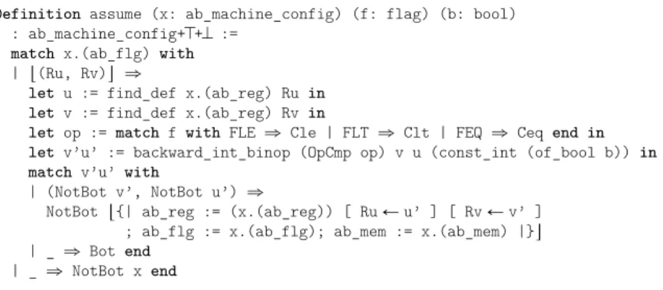
Given such a backward transfer function, assumecan be implemented as shown in Figure 16: if the registersRuand Rvinvolved in the last comparison are known, then the abstract valuesuandvassociated to them can be refined using the backward operator for the given comparison. In case any of these refined values is K, this information is propagated to the whole abstract state: the branch is unreachable and should not be analyzed any further.
Special care has to be taken in the assigntransfer function. If a register that is part of the abstract flag is updated, then no information about its new content can be inferred from the outcome of the comparison. Therefore, in such cases, the abstract flag is simply forgotten, i.e., set to J.
Definition assume (x: ab_machine_config) (f: flag) (b: bool) : ab_machine_config+J+K :=
match x.(ab_flg) with | t(Ru, Rv)u ñ
let u := find_def x.(ab_reg) Ru in let v := find_def x.(ab_reg) Rv in
let op := match f with FLE ñ Cle | FLT ñ Clt | FEQ ñ Ceq end in let v’u’ := backward_int_binop (OpCmp op) v u (const_int (of_bool b)) in match v’u’ with
| (NotBot v’, NotBot u’) ñ
NotBot t{| ab_reg := (x.(ab_reg)) [ Ru Ð u’ ] [ Rv Ð v’ ] ; ab_flg := x.(ab_flg); ab_mem := x.(ab_mem) |}u | _ ñ Bot end
| _ ñ NotBot x end
Figure 16 Implementation of the assume transfer function
This extension of the abstract domain has little impact on the formalization, but greatly increases the precision of the analyzer on programs with conditional branches. Indeed, without this extension, the analyzer cannot deduce anything from the guards of conditional branches as it ignores all comparison instructions.
5.3 A Second Extension: Trace Partitioning
During the execution of a self-modifying program, a given part of the memory may contain completely unrelated code fragments. When these fragments are analyzed, since they are stored at the same addresses, flow sensitivity is not enough to distinguish them. If these fragments are merged in the abstract state, then the two programs get mixed and it is no longer possible to predict the code that is executed with sufficient precision. To prevent such a precision loss, we use a specific form of trace partitioning [22] that makes an analysis sensitive to the value of a particular memory location.
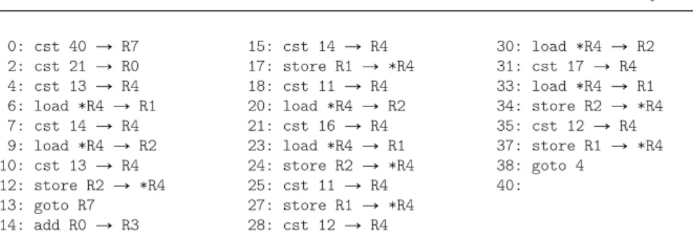
Consider as an example the polymorphic program of Figure 17. Polymor-phism here refers to a technique used by for instance viruses that change their code while preserving their behavior, so as to hide their presence. The main loop of this program (bytes 4 to 39) repeatedly adds forty-two to registerR3(twoadd
instructions at bytes 13 and 14). However, it is obfuscated in two ways. First, the source code initially contains a jump to some random address (byte 13). But this instruction will be overwritten (bytes 7 to 12) before it is executed. Second, this bad instruction is written back (bytes 4 to 6 and 15 to 17), but at a different address (byte 14 is overwritten). The remainder of the loop swaps the contents of memory at addresses 11 and 16, and at addresses 12 and 17 (execution from byte 18 to byte 27, and from byte 28 to byte 37, respectively). So when the execution reaches the beginning of the loop, the program stored in memory is one of two different versions, both featuring the unsafe jump. In other words, this program features two variants that are functionally equivalent
0: cst 40 Ñ R7 2: cst 21 Ñ R0 4: cst 13 Ñ R4 6: load *R4 Ñ R1 7: cst 14 Ñ R4 9: load *R4 Ñ R2 10: cst 13 Ñ R4 12: store R2 Ñ *R4 13: goto R7 14: add R0 Ñ R3 15: cst 14 Ñ R4 17: store R1 Ñ *R4 18: cst 11 Ñ R4 20: load *R4 Ñ R2 21: cst 16 Ñ R4 23: load *R4 Ñ R1 24: store R2 Ñ *R4 25: cst 11 Ñ R4 27: store R1 Ñ *R4 28: cst 12 Ñ R4 30: load *R4 Ñ R2 31: cst 17 Ñ R4 33: load *R4 Ñ R1 34: store R2 Ñ *R4 35: cst 12 Ñ R4 37: store R1 Ñ *R4 38: goto 4 40: Figure 17 Polymorphic program
and look equally unsafe. And running any version changes the program into the other version.
When analyzing this program, the abstract state computed at the beginning of the loop must over-approximate the two program versions. Unfortunately it is not possible to analyze the mere superposition of both versions, in which the unsafe jump may occur. The two versions can be distinguished through, for instance, the value at address 12. We therefore prevent the merging of any two states that disagree on the value stored at this address. Two different abstract states are then computed at each program point in the loop, as if the loop were unrolled once.
More generally, the analysis is parameterized by a partitioning criterion
δ: ab_mc Ñ K that maps abstract states to keys (of some typeK). No abstract states whose keys differ according to this criterion are merged. Taking a constant criterion amounts to disabling this partitioning. The abstract interpreter now computes for each program point a map from keys to abstract states (rather than only one abstract state).
Definition vpAbEnv : Type := (Map [ addr, Map [ K, ab_mc ] ] * int7+K).
Such an environment E represents the following set of machine configurations (ignoring the halted configurations represented by the second component):
γpEq “ tc Pmachine_config| Dk, c P γ ppfst Eqrc.(pc)srksqu
This means that the actual key under which an abstract state is stored has no influence on the concrete states it represents. It can only improve the precision: if two abstract states x and y are mapped to different keys hence not merged, they can represent the concrete set γpxq Y γpyq which may be smaller than
γpx \ yq.
For instance, the criterion used to analyze the polymorphic program of Figure 17 maps an abstract state m to the value stored at address 12 in all concrete states represented by m; or to an arbitrary constant if there may be many values at this address.
To implement this technique, we do not need to modify the abstract domain, but only the iterator and fixpoint checker. The worklist holds pairs (program point, criterion value) rather than simple program points. The iterator and fixpoint checker (along with its proof) are straightforwardly adapted. The
cst -1 Ñ R7 load *R7 Ñ R0 cst key+1 Ñ R6 cst 1 Ñ R1 cst 1 Ñ R2 loop: cmp R1, R0 gotoLE last cst 1 Ñ R7 add R7 Ñ R1 cst 0 Ñ R3 add R2 Ñ R3 key: cst 0 Ñ R4 add R4 Ñ R2 store R3 Ñ *R6 goto loop last: halt R2 Figure 18 Fibonacci
safety checker does not need to be updated since we can forget the partitioning before applying the original safety check.
Thanks to this technique, we can selectively enhance the precision of the analysis and correctly handle challenging self-modifying programs: control-flow modification, mutual modification, and code encryption [14]. However, the analyst must manually pick a suitable criterion for each program to analyze; the analyzer itself is not able to figure out what criterion to use. In practice, we have used the contents of some particular register or memory location.
When using this extension, the termination of the analysis may not be guaranteed any longer as the typeKmay have infinitely many values (or too many for the analysis to enumerate them all). To ensure termination, Kinder [22] proposes a widening operator that merges keys at a particular program point when the number of different keys encountered at this program point exceeds some threshold. We did not implement such a widening operator and require the analyst to be careful when the partitioning criterion is designed.
5.4 A Third Extension: Abstract Decoding
The program in Figure 18 computes the nth Fibonacci number in registerR2,
where n is an input value read from address ´1 and held in register R0. There is a for-loop in which registerR1goes from 1 to n and some constant value is added to registerR2. The trick is that the actual constant (which is encoded as part of an instruction and is stored at the address held inR6) is overwritten at each iteration by the previous value ofR2.
When analyzing this program, we cannot infer much information about the content of the patched cell. Therefore, we cannot enumerate all instructions that may be stored at the patched point. So we introduce abstract instructions: instructions that are not exactly known, but of which some part is abstracted by a suitable abstract domain. Here we only need to abstract values using a numeric domain: the resulting instruction set is shown in Figure 19. This abstraction of the instructions could be pushed further to capture other self-modification patterns. For instance a program might modify only the encoding of a register; in such a case, the “register” part of the instructions could be abstracted by a finite set of registers.
With such a tool, we can decode in the abstract: the analyzer does not recover the exact instructions of the program, but only the information that
Inductive ab_instruction (int7: Type) : Type :=
| AICst (v:int7) (dst:register) | AICmp (src dst: register)
| AIBinop (op: int_binary_operation) (src dst: register) | AILoad (src dst: register) | AIStore (src dst: register) | AIGoto (tgt: int7) | AIGotoInd (r: register)
| AIGotoCond (f: flag) (tgt: int7) | AISkip | AIHalt (r: register).
Figure 19 Abstract instructions
cst 0 Ñ R5 cst j+1 Ñ R0 cmp R5, R6 gotoLE h store R7 Ñ *R0 j: gotoLE 0 h: halt R5 Figure 20 Not-a-branch (* ... slice of ab_post_single ... *) | (AIGotoCond f tgt, sz) ñ
bot_cons (Run (pp + sz)) (T.(assume) m f false) match T.(assume) m f true with
| NotBot m’ ñ
matchconcretize tgt with | Just tgt ñ IntSet.fold
(λ acc addr, Run addr m’ :: acc) tgt nil | All ñ GiveUp :: nil
end | Bot ñ nil end
Figure 21 Abstract conditional jump
some (unknown) value is loaded into registerR4, which is harmless (no stores and no jumps depend on it).
This self-modifying code pattern, in which only part of an instruction is overwritten occurs also in the vector dot product example [14] where specialized multiplication instructions are emitted depending on an input vector.
For this technique to be effective, the numeric abstract domain has to support it: mapping abstract values to abstract instructions (i.e., abstract decoding) should be more efficient than just enumerating all concrete values.
The abstract semantics (Figure 10) has to be slightly modified to deal with this new instruction set. In particular, all jumps behave like indirect jumps: their targets are only known as abstract values. For the analysis to follow such a jump, all concrete destinations need to be enumerated. However, consider the example shown Figure 20: it compares an input value (held in registerR6) to zero, and depending on the outcome, either terminates, modifies itself and then terminates. The conditional jump on linejis unsafe: its target is overwritten on the line before with some input value (the contents of register R7). But the whole program is actually safe, because the branching condition is always false5. Therefore, the abstract transformer for conditional jumps (Figure 21)
tries to prove that the branch cannot be taken before it enumerates its possible targets; and the program of Figure 20 can be proved safe by our analyzer.
5 Such spurious branching instructions are known as “opaque predicates” and used mainly
Program Result Comment Opcode modification X
Multi-level run-time code gen. X
Bootloader × needs a model of system calls and interrupts Control-flow modification X partitioning on the jump target (address 15) Vector dot product X partitioning on loop counter (register R0); andabstract decoding Run-time code checking X
Fibonacci X abstract decoding Self-replication × code segment is “infinite”
Mutual modification X partitioning on the instruction to write (heldin register R0) Polymorphic code X partitioning according to the different versionsof the program (e.g., address 12) Code obfuscation X
Code encryption X partition on the loop counter (register R0) Figure 22 Summary of self-modifying examples
5.5 Summary of the Case Studies
The techniques presented here enable us to automatically prove the safety of various self-modifying programs including almost all the examples of Cai et
al. [11] as summarized in Figure 22. Out of twelve, only two cannot be dealt
with. The comment column of the table lists the extensions that are needed to handle each example (if any), or the limitation of our analyzer. The boot loader example does not fit in the considered machine model, as it calls BIOS interrupts and reads files. The self-replicating example is a program that fills the memory with copies of itself: the code, being infinite, cannot be represented with our abstract domain. Our Coq development [14] features all the extensions along with their correctness proofs, and several example programs including the implementation of the programs listed in Figure 22.
6 Related Work
Most of the previous works on mechanized verification of static analyzes focused on standard data-flow frameworks [23, 15, 4, 10] or abstract interpretation for small imperative structured languages [3, 8, 27]. Klein and Nipkow instantiate such a framework for inference of Java bytecode types [23]; Coupet-Grimal and Delobel [15] and Bertot et al. [4] for compiler optimizations, and Cachera et
al. [10] for data-flow analysis.
The first attempt to mechanize abstract interpretation in its full generality is Monniaux’s master’s thesis [24]. Using the Coq proof assistant and following the orthodox approach based on Galois connections, he runs into difficulties with α abstraction functions being nonconstructive, and with the calculation of abstract operators being poorly supported by Coq. Later, Pichardie’s Ph.D. thesis [30, 28] mechanizes the γ-only presentation of abstract interpretation that we use.