HAL Id: hal-02909189
https://hal.archives-ouvertes.fr/hal-02909189
Submitted on 18 Sep 2020
HAL is a multi-disciplinary open access
archive for the deposit and dissemination of sci-entific research documents, whether they are pub-lished or not. The documents may come from teaching and research institutions in France or abroad, or from public or private research centers.
L’archive ouverte pluridisciplinaire HAL, est destinée au dépôt et à la diffusion de documents scientifiques de niveau recherche, publiés ou non, émanant des établissements d’enseignement et de recherche français ou étrangers, des laboratoires publics ou privés.
Direct numerical simulations of fluids mixing above
mixture critical point
Antoine Michael Diego Jost, Stéphane Glockner, Arnaud Erriguible
To cite this version:
Antoine Michael Diego Jost, Stéphane Glockner, Arnaud Erriguible. Direct numerical simulations of fluids mixing above mixture critical point. Journal of Supercritical Fluids, Elsevier, 2020, 165, pp.1-12. �10.1016/j.supflu.2020.104939�. �hal-02909189�
Direct numerical simulations of fluids mixing above mixture critical point
Antoine Michael Diego Jost1, Stéphane Glockner1, Arnaud Erriguible1,2*
1 Bordeaux INP, University of Bordeaux, CNRS, Arts et Metiers Institute of Technology, INRAE, I2M Bordeaux, F-33600 Talence, France
2 Bordeaux INP, CNRS, University of Bordeaux, ICMCB, F-33600 Pessac, France
*Corresponding author: [email protected]
Direct numerical simulations are performed to quantify the mixing performance of reactors commonly used for crystallization assisted by supercritical fluid above the mixture critical point. Two different reactors are tested: the semi-continuous reactor of milliliter volume range and the continuous microfluidic chip of nanoliter volume range. The current work shows that high performance computing (HPC) is a modern tool useful to analyze various designs and to quantify performances in chemical engineering. In-depth discussions on the numerical methods chosen to strike a good compromise between accuracy and CPU time are presented. Physical analysis is also conducted with an emphasis on the turbulent mixing performance of the reactors. The results show a good mixing for the supercritical technologies considered and underline the increased mixing performance of the microfluidic chip.
1. Introduction
The accurate comprehension of the crystallization processes with a supercritical fluid antisolvent needs a detailed understanding of hydrodynamic phenomena. This process consists on the fast mixing of a solute/solution mixture with an antisolvent to induce high levels of supersaturation. Since nucleation and particle growth occur at molecular diffusion microscales, also known as the Batchelor scale, the solution (solvent + solute) and the turbulent mixing of the antisolvent at this scale are necessary for an in-depth comprehension of supersaturation, the driving force of crystallization. If the smallest resolved scales are greater than those of turbulent mixing, a detailed understanding of the phenomena occurring during the SAS processes is hard to attain since the micromixing occurs at the range of scale around or smaller than the Kolmogorov length scale. At this stage, because of vanishing turbulent fluctuations the smallest eddies are deformed through viscous dissipation and the mixing rate is proportional to √𝜐𝜀, where is the fluid kinematic viscosity and is the turbulent kinetic energy dissipation rate. Its characteristic time is known as the engulfment time constant which was first proposed by Baldyga and Bourne [1]. Consequently, a deep understanding of hydrodynamics effects in supercritical reactors needs to include the mixing smallest scales, namely the Batchelor and the Kolmogorov scales.
For a better understanding of the influence of the hydrodynamic phenomena in the SAS process, experimental studies have been carried out by optical analysis of the fluid mixing in SAS reactors for sub and supercritical conditions. Jet dynamics of pure solvent and solution (with solute) have qualitatively revealed fluid mixing behavior around the mixture critical point [2,3]. From these observations it has been noticed that when the fluid mixture is in a completely miscible zone above the mixture critical point the two fluids have a better mixing, which in turns provides a higher supersaturation degree necessary to the creation of even smaller particles. Despite these promising qualitative results, no quantitative data (especially at the smallest scales) have been obtained to clearly demonstrate the mixing performance of the supercritical process. As mentioned above, the mixing hydrodynamics at molecular diffusion microscales are essential to understand and control the SAS process. Recently, Bassing and Braeuer [4] proposed an experimental technique to capture the micromixing of compressed CO2 and ethanol directly through a one-dimensional in-situ Raman spectroscopy approach. This technique emphasizes the role of micromixing in the case of the ethanol/carbon dioxide mixture. Despite these interesting experimental studies, it is very complicated to determine the effect of the numerous process parameters, or yet, to quantify the mixing performance of the reactor. For these reasons, it is crucial to couple the experimental and numerical studies. This coupling would provide access, at very small scales, to important discrete temporal and discrete spatial data. Although a few numerical studies have been proposed for studying mixing in supercritical crystallization processes [5–7], they are predominantly based on the Reynolds-averaged Navier-Stokes (RANS) governing equations and require turbulence closure models, thereby preventing them from capturing all the mixing scales even when coupled with a micromixing model [8]. It then becomes essential to propose a numerical approach able to accurately determine the values for the hydrodynamic variables for all scales to quantify the mixing performance of the reactor. Nowadays, with the development of supercomputers, direct numerical simulations that resolve all the scales relevant to the mixing physics can be performed. High performance computing (HPC) is, therefore, a modern tool for the further understanding of these processes and results in very satisfactory qualitative and quantitative results.
To demonstrate the potential of HPC for reactor design and the analysis of the performance of the supercritical processes, we investigate the mixing in two types of reactors used for supercritical antisolvent crystallization: the semi-continuous reactor (classic SAS process) and the high pressure microreactor (SAS process). The semi-continuous reactor has been used for decades and has proven its efficiency especially for drug nano/micro-particles synthesis [9]. On the other hand, the microreactor uses the more recent technology of a high pressure microfluidic system. The combination of SCFs and microfluidic reactors (µSAS) can greatly improve the performance and reproducibility of antisolvent processes, as shown in the previous work for conducting organic polymer nanoparticles [10]. More recently, Zhang et al. [11] have proven that turbulent conditions can be achieved in high pressure
microfluidic devices, resulting in ultra-fast mixing times, on the order of 10-4-10-5s, which are highly favorable for synthesizing organic nanoparticles.
In this paper, a significant part is devoted to the presentation of the numerical code Notus [12] (https://notus-cfd.org). We focus primarily on the latest developments that ensure a good balance between accuracy and CPU time in order to perform direct numerical simulations (DNS) on several thousand processors. In the results section, we analyze the turbulence spectra for each case to validate that all flow scales are resolved in order to conduct accurate physical analysis of the mixing. Finally, the mixing performance of the two reactors, determined through their characteristic micromixing times, is quantitatively estimated and compared.
2. Physical model
The system ethanol (solvent) / CO2 (antisolvent) is used for the current study with the fluid being completely miscible for the chosen operating conditions (40°C and 100 bar). It has been shown [13] that in conditions of mixing of CO2 and ethanol above the mixture critical point, the enthalpy of mixing could have important effects. In a previous study, the numerical results obtained by neglecting thermal effects and for the same operating conditions as those currently considered are validated against microPIV experiments [14]. The numerical results were in very good agreement with the experimental results. As such, the hydrodynamic Navier-Stokes equations for a completely isothermal and miscible fluid [14–16] are currently considered. It should be noted that the fluid is far from the mixture’s critical point so the isothermal compressibility is relatively low (between 10−8 and 10−9 Pa−1). Even though the density varies, as it strongly depends on the composition of the mixture, the thermo-compressible effects can be neglected. We have shown that for the current conditions the incompressible and compressible formulations [17] yield results with negligible differences and may be used interchangeably. As for the CFD code currently used the needed CPU time is significantly lower when solving the incompressible formulation, we consider the governing equations for a single phase incompressible flow of a fluid mixture. Simulations are performed for two different geometries of reactors with very different length scales: the semi-continuous reactor with a “large” volume and the microchip reactor. Gravity, neglected in the confined microchip because of the small value of the Bond number, is only considered in the semi-continuous reactor. One of the originalities of the proposed approach is to perform direct numerical simulations (DNS), which solves the governing equations at all scales ranging from the Kolmogorov to the integral length scales, thereby not requiring any turbulence models [11]. The governing equations are the Navier-Stokes equations which follow,
where p is the pressure, ρ is the density of the fluid, g is the gravity vector, µ is the dynamic viscosity, t is the time, and u is the velocity vector. The Peng Robinson equation of state (PR-EOS) with Van der Walls quadratic mixing rules is used to calculate the density of the fluid. The viscosities of the pure fluids, CO2 [18] and ethanol [19], are obtained from the NIST database for the conditions currently considered and viscosity of the mixture is calculated with the classical logarithmic mixing rules [11].
At the inflow boundary, the streamwise velocity component ux has a constant profile in the
coflow and a laminar Poiseuille flow profile for the injector. To speed up the transition to fully turbulent flow uniformly distributed fluctuations ranging between ±0.05 ux are superimposed on the coflow
velocity profiles [20]. A zero-gradient boundary condition is applied at the outlet boundary and no-slip boundary conditions at the remaining boundary conditions.
Recent studies have shown that non-ideal diffusion could be significantly close and above the critical point [21], especially for high temperature and for diffusion controlled flows. Zhang [22] has shown that for the current operating conditions, which are dominated by strong convective flows and low temperature, the non-ideal diffusion considered by the classical Stephan Maxwell model had no effect on the evolution of the mixing in our system. As such, the evolution of each species is calculated by resolving the species conservation equation with advection and ideal diffusion, which follows
where xs is the mass fraction of the solvent and Ds is the diffusion coefficient of the solvent in CO2
calculated by the Hayduck and Minhas correlation [11]. The mass fraction is set to 1 in the injector, 0 in the coflow, and Neumann boundary conditions are applied at the remaining boundary conditions.
3. Numerical methods and optimization
Although Notus code predominantly uses a 2nd order implicit discretization approach, select high order explicit spatial discretizations can be used [25]. Despite the many advantages of an implicit discretization, this approach may pose significant performance penalties for applications whose time step is not limited by numerical stability but by the time scale of the underlying physical phenomena, such as the multi-species coflow micro injector of supercritical fluids in a trapezoidal channel [11,14]. It should be noted that these time step restrictions may be stringent enough that the flows can be
𝛻 ⋅ 𝒖 = 0, (1) 𝜌 (𝜕𝒖 𝜕𝑡+ 𝒖. 𝜵𝒖) = −𝛻𝑝 + 𝛻 ⋅ (𝜇(𝜵𝒖 + 𝜵 𝒕𝒖)) + 𝜌𝒈, (2) 𝜌𝜕𝑥𝑠 𝜕𝑡 + 𝛻 ⋅ (𝜌𝑥𝑠𝒖 + 𝜌𝐷𝑠𝛻𝑥𝑠) = 0, (3)
comprehensive optimization is performed that includes a re-evaluation of the spatial discretization schemes to obtain an appropriate balance between accuracy and efficiency, a reformulation of the variable coefficient Poisson equation in the incompressible Navier-Stokes projection methods, thorough trace and profile analyses to identify computational imbalances and bottlenecks, and a generalized optimization of the MPI communications.
3.1 Time discretization and velocity-pressure solving
The incompressible Navier-Stokes governing equations discussed in Section 2, are solved on a Cartesian staggered grid with a pressure-correction method [23]. For the forward Euler time discretization method, the predictor step follows
where u* is the predicted velocity vector that does not satisfy the incompressibility constraint and Δt is
the time step. The correction step ensures that the solenoidal velocity field follows
where 𝜙𝑛+1= 𝑝𝑛+1− 𝑝𝑛 is the pressure increment. The corresponding boundary conditions between
velocity and pressure increment is the following: where a Dirichlet boundary condition is set to velocity, a Neumann one is set to pressure increment; where a Neumann boundary condition is set to velocity, a Dirichlet one of zero is set to pressure increment.
The scalar transport equation for the mass fraction is subsequently solved on the staggered grid with the velocity un+1 and with the forward Euler time discretization. Finally, ρn+1, μn+1, and D
sn+1 are
updated thanks to PR_EOS and NIST database.
3.2 Spatial discretization
Unlike the universally accepted 2nd order central difference discretization for the variable coefficient diffusion operators [24], the explicit discretization of the advection term of the species transport equation and the non-linear convective term of the momentum equation is application dependent. The challenging task on the choice of the discretization scheme is to attain a good balance between performance and 𝜌𝑛 𝒖∗−𝒖𝒏 𝛥𝑡 + 𝜌 𝑛𝒖𝒏. 𝛁𝒖𝒏= −𝛻𝑝𝑛+ ∇ ⋅ (𝜇𝑛(𝛁𝒖𝒏+ 𝛁𝒕𝒖𝒏)) + 𝜌𝑛, (4) 𝛻 ⋅ (𝛥𝑡 𝜌𝑛𝛻𝜙 𝑛+1) = 𝛻 ⋅ 𝒖∗, (5) 𝒖𝒏+𝟏= 𝒖∗− 𝛥𝑡 𝜌𝑛𝛻𝜙𝑛+1, (6)
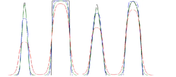
accuracy. This compromise becomes increasingly important and difficult as the size of the computational grid and complexities of the flow features that need to be accurately simulated increases. As such, the high resolution 2nd order total variation diminishing (TVD) centrally discretized scheme with 2nd order symmetric flux-limiters and Lie-Trotter splitting [21], used in high order shock-capturing research codes [25], is deemed a suitable candidate and is implemented in the present work. As shown in Figure 1, for the scalar advection of various discontinuities and smooth features the high resolution TVD scheme with a superbee limiter is significantly more accurate than the WENO-3Z scheme and is slightly less accurate than the WENO-5Z scheme2. For the DNS of the present work, the use of the high resolution TVD scheme for both the advection term in the scalar transport equation and the non-linear convective term in equation (4) and solving a fully explicit formulation of equation (4) results in speed-ups of up to ~8 with no noticeable difference in the time averaged fields required to comprehensively analyze and characterize the quality of the mixing (e.g. mixing index)3.
Figure 1: Scalar advection of smooth and sharp features for various explicit spatial discretization schemes. Black line: reference solution; Green line: WENO-5Z; Red line: WENO-3Z; Blue line: 2nd order TVD scheme with a superbee limiter.
3.3 Variable Coefficient Poisson Equation
Regardless of the spatial discretization schemes used for the explicit predictor step, the Poisson equation (5) of the pressure-correction methods must be solved with a linear solver. For the present work, the iterative methods of BiCGStab(2) (or GMRES) with the geometric multigrid preconditioner PFMG of the high performance preconditioners and solvers library Hypre [26] is used. This computationally intensive calculation may be further complicated by a non-constant coefficient matrix, as is obtained with the current non-uniform density formulation. To reduce the impact of this computationally intensive calculation, the approach proposed by Dodd and Ferrante [27] for the Chorin pressure-correction method is extended to the pressure increment Poisson equation (5). As a result, the variable coefficient matrix is reformulated into a constant coefficient matrix following,
2 The decrease in accuracy of the WENO-3Z scheme, compared to the TVD scheme, is surprising as the former and latter are 3rd and 2nd order accurate, respectively, in space.
3 It should be noted that the current TVD scheme is able to yield such promising speed-ups partly as it does not require a multi-step strong stability preserving time discretization as the WENO-Z schemes.
where ρo = min(ρn). The resulting Poisson pressure increment equation follows,
where a seven-cell stencil central discretization is used for the 3D Laplacian operator 𝛥𝜙.
Similar to Dodd and Ferrante [27] this approach yields significant performance increases. For the present work, speed-ups of up to ~3 are achieved for 32 cores on a grid size of 5.4 × 10⁶ cells.
3.4 Immersed boundary
As Notus only uses Cartesian or rectilinear grids it relies on immersed boundary methods (IBMs) to accurately simulate flow through or past geometries [28,29]. First developed by Peskin and extensively used in numerical simulations of complex geometries, the term IBM refers to any numerical method that discretizes the governing equations on grids that do not conform to the boundary of the desired geometry [30], i.e. non-body conformal grids4. In the pursuit of a compromise between efficiency and accuracy, a 1st order penalization is used which consists on applying the IBCs to a whole cell when its cell center is located inside the immersed domain. The IBCs are implemented in the pressure correction method by setting, in equations (5) and (6), the coefficient Δt/ρn to zero on edges located at the interface between
fluid and solid.
To further speed up the correction step, Frantzis and Grigoriadis [31] proposed further modifications to equation (8) for immersed boundary methods, herein denoted as the FG method. The spirit of the method is to avoid applying the Neumann boundary condition of pressure increment on the immersed interface. Even if it is not mathematically consistent, it is shown in [31] that, with minor adaptation, the solution remains very close to the unmodified system ones. In the present work, a modification to this method is implemented, wherein the RHS of equation (8) and equation (6) as solved on the whole domain including inside the immersed subdomain, and results in time averaged fields with no noticeable difference compared to not applying the modified FG method. It should be noted that when the modified FG method is used additional speed-ups up to ~1.8 are achieved on a grid size of 4.0 × 10⁶ cells.
4 Depending on the approach pursued to implement the immersed boundary conditions (IBCs) the IBMs are characterized as either a direct or continuous forcing method. The reader is encouraged to refer to the review of IBMs by Mittal and Iaccarino [30] for more in-depth discussions on the various IBMs.
𝛻𝜙𝑛+1 𝜌𝑛 → 𝛻𝜙𝑛+1 𝜌𝑜 + ( 1 𝜌𝑛− 1 𝜌𝑜) 𝛻𝜙 𝑛, (7) 𝛥𝜙𝑛+1= 𝛻 ⋅ [(1 −𝜌𝑜 𝜌𝑛) 𝛻𝜙 𝑛] +𝜌𝑜 𝛥𝑡𝛻 ⋅ 𝒖 ∗, (8)
3.5 MPI Optimization & Scalability
As Notus uses a structured grid approach it can take advantage of efficient and straightforward parallel computing algorithms for grid partitioning, load balancing, and MPI communication. The ideal parallelization of a code is the partitioning of the computational domain amongst the processor cores such that each core requires the same amount of time to complete its assigned calculations (perfect load balance), only needs to send/receive data from other cores at the beginning of its assigned calculations (i.e. minimize the number of times of the cores needs to communicate), and minimizes the amount of data sent/received5.
Although Notus is massively parallel and provides an optimized robust MPI parallel framework [12], the large number of MPI processes required for the current work encourages a further optimization with an emphasis on MPI communication. To this end the trace and profiling tools of Extraer and ScoreP, respectively, are used to streamline the various MPI communications and to pursue a general optimization of function calls and structure. A reorganization of the MPI communication routines for the velocity components results in a decrease in the percentage of time spent in MPI_WAIT routines and thus an improvement in the parallel performance and a decrease in computational time of ~8%. It should be noted that a further ~5% decrease in computational time is also achieved by calling the Hypre solver set-up needed for constant coefficient matrix at the first time iteration only.
To comprehensively characterize the parallel behavior of a numerical simulation code it is customary to analyze its strong, strong in-node, and weak scaling.6As shown in Figure 2a, incorporating the proposed optimizations yields significant improvements in the strong in-node scaling. It shows that the optimized Notus has a strong in-node scaling behavior close to that of the theoretical linear for up to 12 cores (~763 cells/core) and for 32 cores (~553 cells/core) it is ~2.5 times faster than the non-optimized
Notus. It should be noted that the pursued optimizations also significantly increase the efficiency from
~30% to ~75% for 32 cores. Achieving higher in-node speed-up is a well know problem and difficult to achieve due to memory bandwidth limitations.
Figure 2b shows the weak scaling wherein the optimized Notus can achieve maximum speed-ups of up to ~19 and ~27, respectively, for 1024 cores. Weak scaling is also improved since slope of the curves are smaller. We can also notice for the optimized version that a slight decrease in efficiency seen
5 It should be noted that achieving a good balance between these, at times conflicting, criteria is the subject of extensive active research. In Notus, the structured grid lends itself to use the efficient Cartesian domain decomposition and allows a good balance between load balance and amount of communicated data (bytes sent/received amongst the cores), while the use of efficient numerical methods and linear solvers decreases the amount of times the cores need to communicate.
6 Strong, and by extension strong in-node, scaling maintains a constant grid size and progressively doubles the number of cores, starting from 1 core (or 1 node for very large mesh sizes). It the total number of cores is limited to those inside a single node, this is defined as strong in-node scaling, while if the total number of cores used exceeds this limit it is defined as strong scaling. An efficient parallelization of a code is synonymous to linear CPU time speed-up as the number of core increases. On the other hand, weak scaling refers to maintaining a constant number of cells per core and progressively increasing the number of cores to eventually span many nodes. An efficient parallelization is synonymous of constant CPU time as the number of core increases.
in the strong in-node scaling as the number of cells per core decrease is also observed for the weak scaling. Lastly, this decrease in efficiency as the number of cells per core decreases is also seen for a strong scaling study on a significantly larger grid size of 300 × 106 cells. Table 1 shows that as the number of cells per core decrease from ~583 to 463, the efficiency of Notus experiences a significant drop from ~89% to ~73%. As the smallest total run time is achieved by using the most cores possible without a performance penalty and maximum efficiency is attained by increasing the number of cells per core, a compromise between these conflicting conditions is necessary
Figure 2: (a) Strong scaling speed-up for a grid size of 1200 × 50 × 90 and (b) weak scaling for 303 and 503 cells per core for DNS of a coflow micro injector with supercritical fluids with a trapezoidal channel. For (a) Red solid line: theoretical values; Black line: pre-optimization; Blue line: post-optimization. For (b) Dashed lines: 303 cells/core; Solid lines: 503 cells/core;
Black line: pre-optimization; Blue line: post-optimization.
Table 1: Strong scaling efficiency for DNS of a coflow micro injector with supercritical fluids in a square channel for a grid size of 300 × 106 cells.
Number of Nodes 4 8 16 32 64
Number of Cores 192 384 768 1536 3072
Number of Cells per Core 116 92 73 58 46
Efficiency (%) 1.00 0.97 0.91 0.89 0.73
4. Results and discussion
As discussed in Section 1 and shown in Figure 3, a large reactor working in a semi-continuous mode and a very small one, a microreactor, working in continuous mode are considered. For the former case, the chosen operating conditions (pressure, temperature, and velocities) are consistent with those commonly used for supercritical antisolvent processes [32]. For the microreactor, the approach of prior studies [11], is pursued and the conditions are such that a very fast mixing is achieved. The characteristic length scales Lc and velocities U used to determine the representative Reynolds numbers (ReC=ρULc/μ)
hydraulic diameter of the channel and its mean velocity, respectively. The Schmidt numbers are calculated according to the mixture viscosities which are determined from the mean ratio of the mass flow rates of the injected fluids (84% and 93%, respectively). The kinematic viscosities for the microreactor and the “large” reactor are 7.95 10-8 m²/s and 6.75 10-8 m²/s, respectively, and the diffusion coefficient is 2.45 10-8 m²/s for both reactors. The operating conditions and relevant non-dimensional numbers for both cases are summarized in Table 1.
Figure 3: Diagrams of the large reactor (left) and microreactor (right).
Table 2. Operating conditions, relevant non-dimensional numbers, and mesh sizes for the microreactor and large reactor
T(K) P(bar) UEtOH(m/s) UCO2(m/s) ReC Sc CO2%mol Nx × Ny × Nz
Microreactor 313.15 100 2.81 3.970 5505 3.25 84 3000 × 430 × 230
Large reactor 313.15 100 3.00 0.001 439 2.75 93 1432 × 520 × 520
DNS simulations require spatial and temporal length scales on the order of the Kolmogorov scale. It has been previously shown that for the current cases the Kolmogorov length scales are on the order of the micrometer [11], the Schmidt numbers are on the order of unity, and the Batchelor scales 𝜆𝐵 =
𝜆𝐾
√𝑆𝑐 are
on the order of the Kolmogorov length scales. This is particularly advantageous for the current numerical simulations as the required resolutions are dominated by the Kolmogorov length scales, i.e. by resolving the flow features at the Kolmogorov length scales we can resolve all mixing scales. Table 1 shows the grid sizes used for the simulations and correspond to a constant grid size of 1 micrometer for the
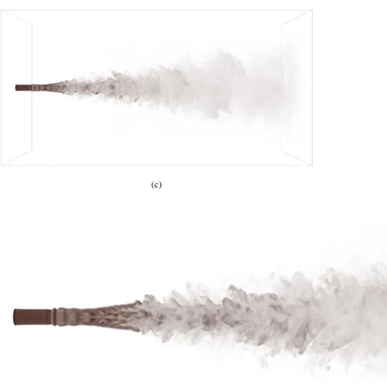
microreactor and a grid size of 7.5 micrometers for a region of size 0.01m × (2.70×10-3)2 m2 placed around the injector for the large reactor. For the latter, a stretched grid is used for the remaining parts of the domain. A good balance between speed-up and efficiency, as previously discussed in Section 3.5, dictates the need for 4096 and 8192 processors for the microreactor and large reactor, respectively, and results in total run times (total CPU time) of approximately 24 and 48 hours for the microreactor and large reactor, respectively. It should be noted that these run times are quite reasonable given the very high resolutions, i.e. large grid sizes, of the simulations. The instantaneous 3D volume renderings of mass fraction for both reactors are shown in Figure 4. Although the complexity of these multiscale flows and the ability to capture the finest details can be appreciated from instantaneous flow field renderings, analysis of additional movies 1 & 2 constructed from successive (in time) instantaneous 3D volume renderings provide a better understanding of the underlying flow phenomena. These turbulent flows are driven by Kelvin Helmholtz (KH) instabilities which are induced by strong shear stress between two layers with different densities (𝜌𝐸𝑡𝑂𝐻
𝜌𝐶𝑂2 = 1.3).
(a)
(c)
(d)
Figure 4: 3D volume renderings of mass fraction (additional material movies 1 & 2) for (a,b) the microreactor and (c,d) the large reactor.
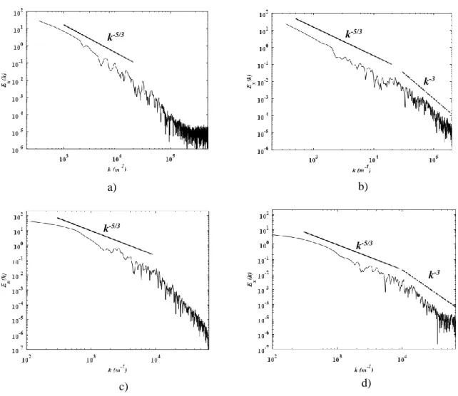
Due to the nature of turbulent flow and the potentially prohibitively large cost of consistently resolving the Kolmogorov length scale, the determination of the smallest resolved scales, and by extension the range of scales resolved, may not be deterministic and instead relies on the analysis of 1D turbulence spectra. To verify that the energy dissipation scales, i.e. the Kolmogorov length scales, are resolved in all the simulations currently pursued, analysis of the 1D turbulence spectra Eu and Ex of the root mean
squared (RMS) velocity and of the fluctuation mass fraction, respectively, are also performed. The root mean squared follows,
where k is the wave number, and ux’ and xs’ are the velocity and mass fraction fluctuations, respectively.
The fluctuation of a variable is defined as the difference between the variable’s instantaneous value and its time averaged, i.e. 𝑢𝑥= 𝑢̅ + 𝑢𝑥′, where 𝑢̅ is the time averaged value. The turbulence spectra are then
obtained by performing a Fast Fourier Transform (FFT) with a Hann window of the desired quantities 〈𝑢𝑥′𝑢𝑥′〉 = ∫ 𝐸𝑢(𝑘)𝑑𝑘 ∞ 0 , (9) 〈𝑥𝑠′𝑥𝑠′〉 = ∫ 𝐸𝑥(𝑘)𝑑𝑘 ∞ 0 , (10)
along the centerline of the domain. Figure 5 shows the spectra up to the Nyquist frequencies, only half of the maximum frequencies to avoid aliasing.
Figures 5a and 5c show the expected Kolmogorov decay of -5/3 for more than two orders of magnitude for the RMS spectra for both reactors. This is widely accepted as a valid indicator of fully developed turbulence and that all relevant length scales for the turbulent flow are resolved, i.e. the resolved length scales range from the energy producing to the energy dissipating scales. Figures 5b and 5d shows that the spectra for the fluctuation of mass fraction follow a slightly different behavior. The inertial-convective region is in good agreement with previous numerical and experimental results and has a slope of -5/3, while the viscous-diffusive range has a larger slope of -3. As previously discussed by Srinivasan [33], the slope for this latter region is more complicated to define and strongly depends on the Schmidt number Sc. In our case, for which Sc = O(1), the slope of this second region is consistent with those of [33,34].
a)
Figure 5: 1D turbulence spectra of (a,b) the microreactor and (c,d) the large reactor for (a,c) velocity RMS and (b,d) mass fraction.
The Q-criterion is widely used to identify and visualize vortices and is derived from the velocity gradient tensor, and follows,
c) d) b) k-5/3 k-5/3 k-5/3 k-5/3 k-3 k-3
where 𝛀 is the vorticity tensor and S is the strain rate which represent the antisymmetric and symmetric parts of the velocity gradient tensor, respectively.
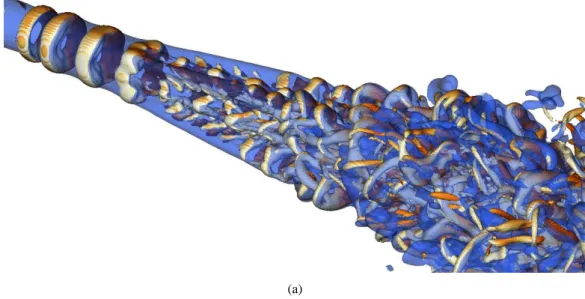
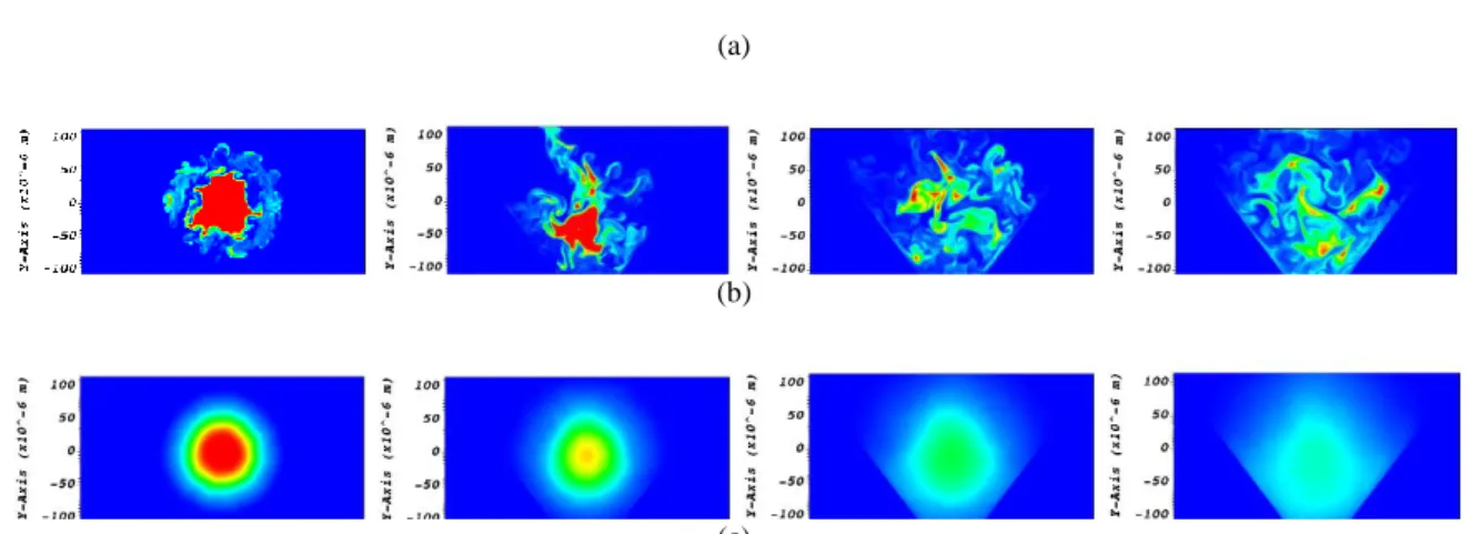
Figure 6a shows the instantaneous isosurfaces for the large reactor simulation for Q = 0.5(UEtOH/DID)
and sheds light on the various stages of transition to fully developed turbulence for coaxial jets. To better characterize the different vortical structures the Q-criterion isosurfaces are colored by one of the transversal vorticity components. Transition is initiated by the development of Kelvin-Helmholtz instabilities which are the result of the shear layer forming due to the density ratio between the jet and the coflow. As seen from Figure 7a, these instabilities result in large ring-forming vortices, hereby denoted as vortex, rings that appear between the internal jet and the quiescent ambient fluid. This is subsequently followed by a region dominated by lateral ejections from the vortex rings which yield series of pinched vortices around the vortex rings [35]. This strong shear layer takes place inside the “conic” spatial extension of the inner and outer edges of the vortex rings. The structures then break into smaller vortices that do not display any preferential direction and the jet becomes a fully developed turbulent jet. This behavior is consistent with previous analyses of coaxial injectors [36]. Transition to turbulence in the coaxial jet of the microreactor follows a different and more drastic behavior. Isosurfaces of Q = 5(UEtOH/DID)2 colored by one of the transversal vorticity components are again used
to identify this intricate behavior. As shown in Figure 6b, although there is only one primary instability at the tip of the injector there are many secondary instabilities on the vortex rings, implying very fast tears of the main structures. This leads to an accelerated transition to turbulence such that at x/DID = 1 the flow is that of fully developed turbulence. Analysis of additional movies 3 & 4 provide a better understanding of the underlying flow phenomena.
(a)
𝑄 =1
2(||𝛀||
(b)
Figure 6: Isosurfaces for Q-criterion colored by the transversal component of the vorticity for the (a) large reactor and (b) microreactor. Additional material movies 3 & 4. In (a) the isosurface of mass fraction are shown in blue.
As shown in Figure 6b, the accelerated transition to turbulence observed in the microreactor leads to a very fast mixing of the solvent and antisolvent. This exceptional mixing is best seen from Figure 7a where an instantaneous evolution of the mass fraction of ethanol and CO2 in the longitudinal plane of the reactor is shown. By also comparing Figures 7b and 7c it can be seen that the ethanol core of the internal jet is particularly short in the streamwise direction. In fact, the evolution of instantaneous and mean mass fraction of the solvent in the transversal planes show that at only x=3DID the species are
already well mixed and at x=11DID a quasi-total mixing is achieved. Further analysis of this mixing will
be presented in the following section.
(a)
(b)
(c)
Figure 7: (a,b) Instantaneous mass fraction of ethanol in the (a) longitudinal plane and (b) transversal plans at (from left to right) x=3DID, 5DID, 7DID, and 11DID for the microreactor. (c) Time averaged mass fraction of ethanol in the transversal
Figure 8 shows the evolution of the mass fraction in the large reactor in both the transversal and longitudinal planes. As shown in Figure 8a, on the longitudinal plane a good mixing between CO2 and ethanol is achieved at a larger x/DID when compared to the microreactor. It should be noted that as shown
in Figures 8b and 8c, the development of secondary instabilities of KH around the core jet induce lateral ejections of the flow, thereby contributing to mixing. Indeed, due to the azimuthal instabilities of the vortex rings, several waves (8 in our case) are formed which coincides with the most predominant instability mode [37]. This phenomenon has been often observed in conventional low pressure conditions but has only recently been observed by Gnanaskandan and Bellan [38] for high pressure conditions, such as those currently pursued.
(a)
(b)
(c)
Figure 8: (a,b) Instantaneous mass fractions of ethanol in the (a) longitudinal plane and (b) transversal plans at (from left to right) x=3DID, 5DID, 7DID, 9DID, and 11DID for the large reactor. (c) Time averaged mass fraction of ethanol in the transversal
planes at (from left to right) x=3DID, 5DID, 7DID, 9DID, and 11DID for the large reactor.
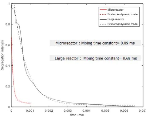
As previously discussed, mixing is one of the predominant mechanisms of the supercritical antisolvent process. To better quantify the efficiency of mixing, the straightforward method detailed in our previous study [11,14] is used to estimate a global mixing time for each reactor. This is considered as the time constant of a function representing the global evolution of the mixing in a reactor which can be easily
modeled by a first order dynamic model (𝑓~𝑒−𝑡−𝑡𝑟𝜏 where and tr are the time constant and the time
delay, respectively). We propose to also consider the global evolution of the well-known segregation index [39] as the parameter chosen to characterize the mixing. The segregation intensity Im is defined
by the following relation:
where 𝑥̅ the spatially averaged mass fraction of the solvent in the yz plane and N the number of nodes 𝑠
in each yz plane. If the segregation tends to one there is a total segregation between species and if it tends to zero, it indicates a perfect mixing. This index is calculated for each abscissa x for the yz plane [14]. In order to determine the time constant for the phenomenon, the evolution of the segregation index is represented as a function of time by transforming the abscissa thanks to the velocity injection of the solvent t = x/ui.. Figure 9 shows the segregation index for both cases and sheds light on the excellent
mixing of both reactors, i.e. the segregation index tends to zero very quickly. The comparison with the first order dynamic model gives a time constant of around 0.09 ms for the microreactor and 0.68 ms for the large reactor.
Figure 9: Evolution of the segregation intensities as a function of the time and comparison with the first order dynamic model for both reactors.
Bassing and Braeuer [4] revealed that micromixing is the predominant mechanism of mixing for such reactors, and consequently we propose to map the local micromixing time in both reactors through the 𝐼𝑚=
∑ (𝑥𝑁1 𝑠−𝑥̅̅̅)𝑠2
relation presented by Baldyga and Bourne [1], 𝑡𝑚= 17.24√ 𝜐
𝜀 . The dissipation rate of the turbulent
kinetic energy ε follows,
(1)
Whereas estimating the value of this crucial parameter needed to determine the local micromixing time is one of the main challenges of experimental approaches, one of the advantages of the present DNS simulations is their ability to quantitatively determine the dissipation rate of the turbulent kinetic energy at all locations in the flow field.
Figure 10 shows the contour maps of the micromixing time in the transversal planes for the two reactors, and as expected, the intense micromixing times are the smallest within the shear layer, delimited in Figure 10.
(a)
(b)
Figure 10: Instantaneous micromixing indices for (a) the large reactor (inverse scale from 1×10⁻⁵ to 2×10⁻³ s) at x= 9D
ID and (b) the microreactor (inverse scale from 1×10⁻⁵ to 2×10⁻³ s) at x= 1D
ID
Figure 11 shows the dispersion of the micromixing times in the meridian plane of the reactors. It can be observed that even though strong mixing zones are present for the large reactor, the microreactor has an important homogeneous zone with shorter micromixing times. The latter region is the result of higher 𝜀 = 2𝜈 [ (𝜕𝑢𝑥′ 𝜕𝑥) 2 + (𝜕𝑣𝑦 ′ 𝜕𝑥) 2 + (𝜕𝑤𝑧 ′ 𝜕𝑥 ) 2 + (𝜕𝑢𝑥 ′ 𝜕𝑦) 2 + 2 (𝜕𝑣𝑦 ′ 𝜕𝑦) 2 + (𝜕𝑤𝑧 ′ 𝜕𝑦 ) 2 + (𝜕𝑢𝑥 ′ 𝜕𝑧) 2 + (𝜕𝑣𝑦 ′ 𝜕𝑧) 2 + 2 (𝜕𝑤𝑧 ′ 𝜕𝑧 ) 2 + 2 (𝜕𝑢𝑥 ′ 𝜕𝑦 𝜕𝑣𝑦′ 𝜕𝑥) +2 (𝜕𝑢𝑥 ′ 𝜕𝑧 𝜕𝑤𝑧′ 𝜕𝑥 ) + 2 ( 𝜕𝑤𝑧′ 𝜕𝑦 𝜕𝑣𝑦′ 𝜕𝑧) ]
dissipation rates for the turbulent kinetic energy. The range of the micromixing times is also consistent with that obtained from the segregation index method indicating, as it has already been proven experimentally [4], that the mixing in such supercritical reactors is governed by micromixing. Finally, it should be emphasized, that regardless of the size of the reactor and as a result of the special properties of the supercritical fluids, the time scales of the mixing are smaller, at times significantly smaller, to those encountered for reactors using more conventional fluids [11].
(a)
(b)
Figure 11: Instantaneous micro mixing indices in the meridian plane for (a) the large reactor and (b) the microreactor.
Finally, in order to compare the mixing performance of the two reactors, the volumetric distribution of the micromixing time for the mixing zone delimited by the dashed black lines on the meridian plane, shown in Figure 11 are compared. Figure 12 shows the percentage of volume affected by the micromixing time range. As previously discussed, the mean times of these distributions are consistent with previous estimates. It should be noted, however, that the shape of these distributions is of greater significance. Whereas a sharp distribution is observed for the microreactor, a large distribution is seen for the large reactor which highlights containment effects due to domain volume reduction. As the spatial and temporal time scales of the microreactor are smaller than those of the large reactor, an increase in mixing performance is achieved.
tm (s)
Figure 12: Volumetric distributions of the micromixing times in the most intense mixing zone for the two reactors.
5. Conclusion
In this paper, direct numerical simulations are performed to analyze the mixing performance of crystallization reactors processing with supercritical fluids. The analysis is conducted for two different reactors, a semi-continuous large reactor and a continuous microreactor. In order to perform simulations on several thousand processors to resolve all the relevant scales of the mixing, the numerical methods of the in-house open-source code Notus are improved to strike a good balance between accuracy and CPU time. The operating conditions, which are above the mixture critical point, result in good mixing for both cases with mixing times inferior than the millisecond. Using the results from the DNS simulations accurate estimates of the micromixing times for very small scales are obtained and indicate that micromixing is the predominant mixing mode in the current supercritical reactors. Finally, the mixing analysis emphasizes that the microreactor outperforms the large reactor. Furthermore, due to the smaller spatial and temporal scales of microreactors greater control of the operating conditions can be achieved. It however should be noted that the mass flow rate (1.04 mg/min) used in the microreactor is much lower than in that used for the large reactor (3.61 mg/min). As a result, even though the microreactor offers excellent mixing performance and better control of the conditions, the large reactor has the big advantage of working with higher mass flow rates. Finally, the essential perspective should be to study the scaling options of the microreactor: can a continuous micro/milli reactor operate at the same flow rates as a large reactor and maintain an excellent mixing performance?
Acknowledgement
We acknowledge the French National Research Agency for its support (ANR-17-CE07-0029 - SUPERFON), and the MCIA (Mésocentre de Calcul Intensif Aquitaine) and GENCI (DARI project number A0062A10815) for their HPC resources.
References
[1] J. Baldyga, J.R. Bourne, Simplification of micromixing calculations. I. Derivation and application of new model, Chem. Eng. J. 42 (1989) 83–92. https://doi.org/10.1016/0300-9467(89)85002-6.
[2] T. Petit-Gas, O. Boutin, I. Raspo, E. Badens, Role of hydrodynamics in supercritical antisolvent processes, J. Supercrit. Fluids. 51 (2009) 248–255. https://doi.org/10.1016/j.supflu.2009.07.013. [3] E. Reverchon, E. Torino, S. Dowy, A. Braeuer, A. Leipertz, Interactions of phase equilibria, jet
fluid dynamics and mass transfer during supercritical antisolvent micronization, Chem. Eng. J. 156 (2010) 446–458. https://doi.org/10.1016/j.cej.2009.10.052.
[4] D. Bassing, A.S. Braeuer, The lag between micro- and macro-mixing in compressed fluid flows, Chem. Eng. Sci. 163 (2017) 105–113. https://doi.org/10.1016/j.ces.2017.01.034.
[5] A. Martı́n, M.J. Cocero, Numerical modeling of jet hydrodynamics, mass transfer, and crystallization kinetics in the supercritical antisolvent (SAS) process, J. Supercrit. Fluids. 32 (2004) 203–219. https://doi.org/10.1016/j.supflu.2004.02.009.
[6] F.A.R. Cardoso, R.V.P. Rezende, R.A. Almeida, H.F. Meier, L. Cardozo-Filho, Effect of precipitation chamber geometry on the production of microparticles by antisolvent process, J. Supercrit. Fluids. 133 (2018) 357–366. https://doi.org/10.1016/j.supflu.2017.09.015.
[7] M.A.T. Cardoso, J.M.S. Cabral, A.M.F. Palavra, V. Geraldes, CFD analysis of supercritical antisolvent (SAS) micronization of minocycline hydrochloride, J. Supercrit. Fluids. 47 (2008) 247–258. https://doi.org/10.1016/j.supflu.2008.08.008.
[8] J. Sierra‐Pallares, D.L. Marchisio, M.T. Parra‐Santos, J. García‐Serna, F. Castro, M.J. Cocero, A computational fluid dynamics study of supercritical antisolvent precipitation: Mixing effects on particle size, AIChE J. 58 (2012) 385–398. https://doi.org/10.1002/aic.12594.
[9] L. Padrela, M.A. Rodrigues, A. Duarte, A.M.A. Dias, M.E.M. Braga, H.C. de Sousa, Supercritical carbon dioxide-based technologies for the production of drug
nanoparticles/nanocrystals – A comprehensive review, Adv. Drug Deliv. Rev. 131 (2018) 22–78. https://doi.org/10.1016/j.addr.2018.07.010.
[10] R. Couto, S. Chambon, C. Aymonier, E. Mignard, B. Pavageau, A. Erriguible, S. Marre, Microfluidic supercritical antisolvent continuous processing and direct spray-coating of poly(3-hexylthiophene) nanoparticles for OFET devices, Chem. Commun. 51 (2014) 1008–1011. https://doi.org/10.1039/C4CC07878K.
[11] F. Zhang, S. Marre, A. Erriguible, Mixing intensification under turbulent conditions in a high pressure microreactor, Chem. Eng. J. 382 (2020) 122859.
https://doi.org/10.1016/j.cej.2019.122859.
[12] Notus CFD code web site: https://notus-cfd.org., (n.d.).
[13] J. Sierra-Pallares, A. Raghavan, A.F. Ghoniem, Computational study of organic solvent–CO2 mixing in convective supercritical environment under laminar conditions: Impact of enthalpy of mixing, J. Supercrit. Fluids. 109 (2016) 109–123. https://doi.org/10.1016/j.supflu.2015.11.007. [14] F. Zhang, A. Erriguible, S. Marre, Investigating laminar mixing in high pressure microfluidic
[15] A. Erriguible, T. Fadli, P. Subra-Paternault, A complete 3D simulation of a crystallization process induced by supercritical CO2 to predict particle size, Comput. Chem. Eng. 52 (2013) 1– 9. https://doi.org/10.1016/j.compchemeng.2012.12.002.
[16] A. Erriguible, S. Laugier, M. Laté, P. Subra-Paternault, Effect of pressure and non-isothermal injection on re-crystallization by CO2 antisolvent: Solubility measurements, simulation of mixing and experiments, J. Supercrit. Fluids. 76 (2013) 115–125.
https://doi.org/10.1016/j.supflu.2013.01.015.
[17] S. Amiroudine, J.-P. Caltagirone, A. Erriguible, A Lagrangian–Eulerian compressible model for the trans-critical path of near-critical fluids, Int. J. Multiph. Flow. 59 (2014) 15–23.
https://doi.org/10.1016/j.ijmultiphaseflow.2013.10.008.
[18] A. Laesecke, C.D. Muzny, Reference Correlation for the Viscosity of Carbon Dioxide, J. Phys. Chem. Ref. Data. 46 (2017). https://doi.org/10.1063/1.4977429.
[19] S.B. Kiselev, J.F. Ely, I.M. Abdulagatov, M.L. Huber, Generalized SAFT-DFT/DMT Model for the Thermodynamic, Interfacial, and Transport Properties of Associating Fluids: Application for n-Alkanols, Ind. Eng. Chem. Res. 44 (2005) 6916–6927. https://doi.org/10.1021/ie050010e. [20] G.N. Taub, H. Lee, S. Balachandar, S.A. Sherif, A direct numerical simulation study of higher
order statistics in a turbulent round jet, Phys. Fluids. 25 (2013) 115102. https://doi.org/10.1063/1.4829045.
[21] P. He, A. Raghavan, A.F. Ghoniem, Impact of non-ideality on mixing of hydrocarbons and water at supercritical or near-critical conditions, J. Supercrit. Fluids. 102 (2015) 50–65.
https://doi.org/10.1016/j.supflu.2015.03.017.
[22] F. Zhang, Supercritical Antisolvent (SAS) Process Intensification through the Use of High Pressure (HP) Microfluidic Mixing, Université de Bordeaux, 2019.
[23] K. Goda, A multistep technique with implicit difference schemes for calculating two- or three-dimensional cavity flows, J. Comput. Phys. 30 (1979) 76–95. https://doi.org/10.1016/0021-9991(79)90088-3.
[24] C. Hirsch, Numerical Computation of Internal and External Flows, Volume 2: Computational Methods for Inviscid and Viscous Flows | Wiley, Wiley.Com. (n.d.). https://www.wiley.com/en-us/Numerical+Computation+of+Internal+and+External+Flows%2C+Volume+2%3A+Computati onal+Methods+for+Inviscid+and+Viscous+Flows-p-9780471924524 (accessed April 20, 2020). [25] J. Zhang, T.L. Jackson, A.M.D. Jost, Effects of air chemistry and stiffened EOS of air in
numerical simulations of bubble collapse in water, Phys. Rev. Fluids. 2 (2017) 053603. https://doi.org/10.1103/PhysRevFluids.2.053603.
[26] R.D. Falgout, J.E. Jones, U.M. Yang, The Design and Implementation of hypre, a Library of Parallel High Performance Preconditioners, in: A.M. Bruaset, A. Tveito (Eds.), Numer. Solut. Partial Differ. Equ. Parallel Comput., Springer, Berlin, Heidelberg, 2006: pp. 267–294. https://doi.org/10.1007/3-540-31619-1_8.
[27] M.S. Dodd, A. Ferrante, A fast pressure-correction method for incompressible two-fluid flows, J. Comput. Phys. 273 (2014) 416–434. https://doi.org/10.1016/j.jcp.2014.05.024.
[28] A.M.D. Jost, S. Glockner, Direct forcing immersed boundary method: Improvements to the Ghost Node Method, Submitt. J. Comput. Phys. (2020).
[29] J. Picot, S. Glockner, Reduction of the discretization stencil of direct forcing immersed boundary methods on rectangular cells: The ghost node shifting method, J. Comput. Phys. 364 (2018) 18– 48. https://doi.org/10.1016/j.jcp.2018.02.047.
[30] R. Mittal, G. Iaccarino, Immersed Boundary Methods, Annu. Rev. Fluid Mech. 37 (2005) 239– 261. https://doi.org/10.1146/annurev.fluid.37.061903.175743.
[31] C. Frantzis, D.G.E. Grigoriadis, An efficient method for two-fluid incompressible flows appropriate for the immersed boundary method, J. Comput. Phys. 376 (2019) 28–53. https://doi.org/10.1016/j.jcp.2018.09.035.
[32] C. Neurohr, A. Erriguible, S. Laugier, P. Subra-Paternault, Challenge of the supercritical antisolvent technique SAS to prepare cocrystal-pure powders of naproxen-nicotinamide, Chem. Eng. J. 303 (2016) 238–251. https://doi.org/10.1016/j.cej.2016.05.129.
[33] K.R. Sreenivasan, Turbulent mixing: A perspective, Proc. Natl. Acad. Sci. 116 (2019) 18175– 18183. https://doi.org/10.1073/pnas.1800463115.
[34] F. Plourde, M.V. Pham, S.D. Kim, S. Balachandar, Direct numerical simulations of a rapidly expanding thermal plume: structure and entrainment interaction, J. Fluid Mech. 604 (2008) 99– 123. https://doi.org/10.1017/S0022112008001006.
[35] K. Prestridge, J.C. Lasheras, Three-dimensional vorticity dynamics in a coflowing turbulent jet subjected to axial and azimuthal perturbations, ESAIM Proc. 1 (1996) 553–564.
https://doi.org/10.1051/proc:1996027.
[36] G. Balarac, O. Métais, M. Lesieur, Mixing enhancement in coaxial jets through inflow forcing: A numerical study, Phys. Fluids. 19 (2007) 075102. https://doi.org/10.1063/1.2747680. [37] S.E. Widnall, D.B. Bliss, C.-Y. Tsai, The instability of short waves on a vortex ring, J. Fluid
Mech. 66 (1974) 35–47. https://doi.org/10.1017/S0022112074000048.
[38] A. Gnanaskandan, J. Bellan, Side-jet effects in high-pressure turbulent flows: Direct Numerical Simulation of nitrogen injected into carbon dioxide, J. Supercrit. Fluids. 140 (2018) 165–181. https://doi.org/10.1016/j.supflu.2018.04.015.
[39] P.V. Danckwerts, The effect of incomplete mixing on homogeneous reactions, Chem. Eng. Sci. 8 (1958) 93–102. https://doi.org/10.1016/0009-2509(58)80040-8.