Continuous nonlinear systems

CONTINUOUS NONLINEAR SYSTEMS

DONALD A. GEORGE

TECHNICAL REPORT 355 JULY 24, 1959

MASSACHUSETTS INSTITUTE OF TECHNOLOGY RESEARCH LABORATORY OF ELECTRONICS

The Research Laboratory of Electronics is an interdepartmental laboratory of the Department of Electrical Engineering and the Department of Physics.

The research reported in this document was made possible in part by support extended the Massachusetts Institute of Technology, Research Laboratory of Electronics, jointly by the U. S. Army (Sig-nal Corps), the U.S. Navy (Office of Naval Research), and the U.S. Air Force (Office of Scientific Research, Air Research and Develop-ment Command), under Signal Corps Contract DA36-039-sc-78108, Department of the Army Task 3-99-20-001 and Project 3-99-00-000.

MASSACHUSETTS INSTITUTE OF TECHNOLOGY RESEARCH LABORATORY OF ELECTRONICS

Technical Report 355 July 24, 1959

CONTINUOUS NONLINEAR SYSTEMS

Donald A. George

This report is based on a thesis submitted to the Department of Electrical Engineering, M. I. T., July 24, 1959 in partial fulfill-ment of the requirefulfill-ments for the degree of Doctor of Science.

Abstract

A functional representation, which is a generalization of the linear convolution inte-gral, is used to describe continuous nonlinear systems. Emphasis is placed on nonlinear systems composed of linear subsystems with memory, and nonlinear no-memory subsystems. An "Algebra of Systems" is developed to facilitate the description of such combined systems. From this algebraic description, multidimensional system trans-forms are obtained. These transforms specify the system in much the same manner as one-dimensional transforms specify linear systems. The system transforms and the transform of the system's input signal are then used to determine the transform of the

output signal. Transform theory is also used for determining averages and spectra of the system output when the input is a random signal Gaussianly distributed. Certain theoretical aspects of the functional representation are discussed.

TABLE OF CONTENTS

I. Introduction 1

1. 1 System Analysis 1

1. 2 Functional Representation 1

1. 3 Historical Note 2

1.4 Comparison of the Functional Approach with Other Nonlinear Methods 2

1.5 Interpretation of the Functional Series 4

1.6 System Transforms 7

1. 7 Summary 8

II. An Algebra of Systems 9

2. 1 Introduction 9 2. 2 Functional Operations 10 2. 3 System Combinations 12 2.4 Order of Systems 18 2.5 Special Systems 19 2. 6 Example 1 20 2. 7 Cascade Operations 20 2.8 Feedback Systems 23

2. 9 Impulse Responses and Transforms 27

2. 10 Summary 31

III. System Transforms 32

3. 1 Introduction 32

3. 2 Multidimensional Transforms 33

3. 3 Steady-State Response 39

3.4 Initial-Value and Final-Value Theorems 41

3.5 Example 2 41

3. 6 Example 3 44

3. 7 Example 4 45

3.8 Summary 47

IV. Remark on Applications of the Algebra of Systems and System Transforms 48

4. 1 Block-Diagram Manipulations 48 4. 2 Complex Translation 49 4. 3 A Final-Value Theorem 51 4.4 Delay Theorem 52 4.5 Differentiation Theorem 53 4.6 Limit Cycles 53

4. 7 Measurement of Nonlinear Systems 55

CONTENTS V. Random Inputs 59 5. 1 Introduction 59 5.2 Output Averages 59 5. 3 Gaussian Inputs 60 5.4 Use of Transforms 63 5.5 Example 5 66 5. 6 Example 6 68 5. 7 Optimum Systems 69 5.8 Example 7 72 5. 9 Example 8 73

5. 10 Theoretical Discussion on Measurements 74

5. 11 Summary 75

VI. Theoretical Discussion of Functional Representation 76

6. 1 Domain and Range 76

6. 2 Algebraic Laws 76

6. 3 Feedback and Inverses 78

6. 4 Input-Output Uniqueness 79

6. 5 Functional Taylor's Series 81

6. 6 The Iteration Series 84

6. 7 Continuous Systems 87

6. 8 Conclusion 88

Appendix A. Transforms 89

1. System Transforms 89

2. Association of Variables 90

3. Final-Value and Initial-Value Theorems 91

Appendix B. Problem Details 93

1. Problems of Section 3. 5 93

2. Problems of Sections 3. 6 and 3. 7 95

3. Problems of Section 5.5 96 4. Problems of Section 5. 6 97 5. Problems of Section 5. 9 100 Acknowledgment 101 References 102 iv

I. INTRODUCTION 1.1 SYSTEM ANALYSIS

In physical analysis, a "sysi and an effect. In system termii output. This is represented in

x(t) _NONLINEAR SYSTEM

f(t)

Fig. 1. Nonlinear system.

The continuous concept implies

tem" is nology,

often used to specify the relation between a cause the cause is the system input and the effect is the Fig. 1, where x is the input signal and f is the output signal. Usually these signals are functions of time. Of the several general classifications of systems, the class that has been most successfully studied is the linear, time-stationary system. This report is concerned with the nonlinear, stationary system - particularly the con-tinuous nonlinear stationary system. The concon-tinuous

non-linear system will be described in detail in section 6. 8. a certain degree of smoothness in the system's input-output relation. The linear system can be regarded as a special case of the continuous nonlinear system.

The analysis of a system is dependent upon finding a mathematical description of the relation between the system input and the system output. Classically, the relation is obtained by means of a differential equation. However, the present means of repre-senting a linear system is by the convolution integral and its associated transforms. The mathematical representation for nonlinear systems which forms the basis of this report is closely related to these modern methods for linear system analysis.

1.2 FUNCTIONAL REPRESENTATION

A function f operates on a set of variables x to produce a new set of variables f(x). A functional, however, operates on a set of functions and produces a new set of functions. In other words, a functional is a function of a function.

The mathematical description used in this report to represent a nonlinear system is the functional series:

f(t) = h(T) X(t-T) dT +

h2(T1l

oo 00 0oo

fo

1 ... n (1)

where f(t) is the system output, and x(t) is the system input. The first term in this series is the ordinary convolution integral that is used for linear system analysis. The other terms are generalizations of this linear convolution term. In linear system theory, the function h(t) is known as the "impulse response." In section 1.5, the function

hn(tl .. ., tn) will be shown to be a generalized impulse response. In this report, the

1 !~~~~~~~~~

limits of integration, unless otherwise indicated, will be from -oo to oo. 1.3 HISTORICAL NOTE

These functionals were studied by Volterra (1) early in the twentieth century. In 1942, Wiener (2) first applied the functional series to the study of a nonlinear electrical circuit problem. He was concerned with computing the output moments of a detector circuit with a random input. Later, he used this representation as the basis for a canonical form for nonlinear systems (3).

More recently, the functional representation has been investigated by a number of workers. Bose (3) investigated the canonical form problem and developed a system that overcame many of the difficulties associated with Wiener's system. Brilliant (4) was concerned with the validity of the functional representation, and found that systems

satisfying a certain continuity condition could be represented. He also showed that the representation was well suited to the combining of nonlinear systems.

Wiener and others have extended the application of this functional representation, in the random input case, beyond the results of Wiener's paper of 1942. Wiener (5) developed the rigorous theory for random (white Gaussian) inputs and applied the theory to such situations as are found in FM spectra. Barrett's (6) paper is an excellent

expo-sition of the state of this theory at the time the present work was undertaken.

1.4 COMPARISON OF THE FUNCTIONAL APPROACH WITH OTHER NONLINEAR METHODS

The analysis of nonlinear systems has been an interesting problem for many years. It is therefore of benefit to compare the present state of the functional approach with the principal classical methods. There are two main classes of solutions to nonlinear

prob-lems: transient solutions, and steady-state solutions.

Transient solutions are obtained classically by the solution of nonlinear differential equations (7). For first-order equations, solutions can usually be obtained formally, although numerical integration procedures may be required. However, bnly special forms of second-order equations can be solved. Force-free solutions for second-order equations can be found with the phase-plane method - even for extremely violent nonlin-earities. Examples of violent and nonviolent nonlinearites are shown in Fig. 2. Gen-erally, numerical techniques must be used to solve higher-order equations.

Sinusoidal steady-state solutions can be obtained for systems in which the first harmonic is the only significant term. This is the basis for the "describing function method" (8), and for some others. System order is not a limiting factor, nor, generally, is the violence of the nonlinearity.

The functional series (Eq. 1) is a very general method for representing nonlinear systems (see secs. 2.1 and 6.8). However, at least in the present state of these methods, it does have a definite practical limitation. If the nonlinearities in a system are too violent, the number of terms required for a close approximation becomes very large.

OUTPUT f INPUT x (a) OUTPUT f INPUT x (b)

Fig. 2. Violence of nonlinearities: (a) nonviolent nonlinearity (vacuum tube with "medium" signal); (b) violent non-linearity (ideal clipper).

a W 0 M W 3 2 0 VIOLENCE OF NONLINEARITY (a) 5 4 " 3 0o 2 - I N N EFFECTIVE HARMONICS (b)

Fig. 3. Application graphs: (a) tions. (Unbroken lines representation; broken sical methods.)

transient solutions; (b) steady-state solu-show the region covered by the functional lines show the region covered by the

clas-3

'

::~1_

It would then be necessary to resort to a computer, and a great deal of the value of the method would be lost. However, if the nonlinearities are sufficiently smooth, the trans

-ient response of a system is determined by the first few terms of the series, and there is little limitation from system order. Also, steady-state solutions do not require that the first harmonic be the only significant term.

The comparisons that have just been made are illustrated graphically in Fig. 3. The shaded areas show the regions of effectiveness of various methods of analysis. However, the graphs should not be taken to mean that these methods can cover all systems in the shaded regions, but only a significantly large number.

The first problem in system analysis is to find a suitable mathematical description. This description is called the "system representation." The functional representation studied in this report has three important properties:

(a) It has an explicit input-output relation. (b) It facilitates the combination of systems. (c) It allows the consideration of random inputs.

If a representation has an implicit - rather than explicit - input-output relation, it means that the whole problem must be re-solved for each different input. (The differential equation representation is implicit.) Property (b) is important because the electrical engineer spends a great deal of time "putting things together." The effect of random inputs is a problem of great interest to the engineer.

The classical methods based on the differential equation have none of these proper-ties. On the other hand, the significance of transform and convolution methods in linear system analysis rests heavily on these properties. Therefore, these three properties give three distinct advantages to the functional representation as compared with the classical nonlinear methods.

1.5 INTERPRETATION OF THE FUNCTIONAL SERIES

Having indicated the position of the functional representation in the general field of nonlinear system analysis, the writer would like to present an interpretation of the functional series. First of all, the series (Eq. 1) can be viewed as a series of time functions:

f(t) = fl(t) + f2(t) + ... + fn(t) + ... (2)

where

fn(t)

That is, at some time t1 we have a series of numbers fn(tl) that add up to give the

actual value of the system output f(tl). Also, each of the functions f (t) is seen from Eq. 3 to be the result of a convolution operation on the input time function x(t). The first term, fl(t), in particular, is recognized as being the result of putting x(t) into a

linear system with an impulse response, h(t). Indeed, each term fn(t) can be viewed as the output of a system with input x(t).

To take advantage of this idea, we introduce an operator notation. In this notation, if we have a

gen-x f eral nonlinear system with output f(t) and input x(t), as

illustrated in Fig. 1, then we can write f(t) = H[x(t)], or if we make the time dependence implicit, f = H[x]. Fig. 4. Nonlinear system. Then the symbol H represents the operation that the

system makes on input x to produce output f. In dia-gram form, a nonlinear system is then represented as shown in Fig. 4. (The usual operator notation ' is replaced by H in this report.)

The first term can be viewed as a linear system operation, and therefore fl(t) = Hl[X(t)]

or

fl= H₁[x]

where the subscript "1" is added to the H notation to denote that the operation is linear. Now, a linear system is specified by means of its impulse response; and thus, associated with the linear system H1, there is an impulse response hi(t), and

fl(t) =

f

Now, the second term in the series (Eq. 2) is

f2()

jj

If the input x(t) is changed by a gain factor E to give a new input ex(t), then the new output, g2(t), is g₂(t) =

j

Thus, the second term is the result of a quadratic (or squaring) operation. In the oper-ator notation, then, f2 = H2[x], where the subscript "2" indicates that this is a quadratic

operation. Similarly, = H[x]. f3 H Associated with each Hn

is the function hn(t 1 ... . tn), and

fn(t) = ... h- 1'. Tn ) x(t-T1) . x(t-Tn) dT ldT

In the light of these remarks, Eq. 1 can be rewritten as

f = H[x] + H2[x] + ... + Hn[X] + (6)

That is, the system H has been broken into a parallel combination of systems Hn, as shown in Fig. 5. This is the desired inter-pretation: The functional representation represents a nonlinear system as a par-allel bank of systems H that are nt h

--n

order nonlinear systems and have an impulse -response function hn(t 1' . .. tn) associated with them.

The next task is to show how these functions h (t1, . . .,t ) can be interpreted

as impulse responses. The linear case is well known. If fl = H1l[x], and x(t) =

Fig. 5. Block diagram for the functional 6(t+T), an impulse at time -T, then f(0) = representation.

h1(T), where hl(t) is the impulse response. Now consider a generalization of the second term of the functional series

g₂(t) = h₂ (T1, T2) x(t-T1) Y(t-T 2) dTldT2

and represent this operationally by

g2 = H2 (xy)

(7)

(8) This operational form will be considered in greater detail in section 2. 2. The difference between f₂ = H₂[x] and g2 = H2(xy) should be noted. The square brackets denote an actual

system operation, and the parentheses denote a mathematical operation on a pair of func

-tions. Such a form (Eq. 8) cannot occur by itself because only single-input systems are being studied. However, it can occur in combination with other terms. onsider the

system operation f2 = H2[x+y].

Using Eq. 4 (the actual functional relation) with Eqs. 7 and 8, we obtain f₂ = H₂ (xx) + H₂(XY) + H2(YX) + H2(YY)

but h₂(t₁, t₂) is a symmetrical function, and so

f = H2(x2) + 2H2(xy) + H2(y2) (9)

where xx = x and yy = y . In the functional form for the second-order case (Eq. 7), with hl(tl, t₂) # h₂(t₂, tl), the symmetrical function [h2(tl, t2)+h2(t2, t1)] /2 can be formed

and substituted for h₂(t₁, t₂) without affecting f2(t). This procedure (5) generalizes to

hn(tl, .. .. tn), and so it will generally be assumed in this report that hn(tl . . i tn) is a

symmetrical function in t, t2, ... , tn _.

In Eq. 9, H2(xy) has been obtained, but it is in combination with two other terms.

Figure 6 shows how H_{2(xy) can be isolated experimentally. If the indicated operations} were performed sequentially, only one system H2 would be needed. In the system

y(T

v(t

of Fig. 6, if x(t) = 6(t+T1) and y(t) = 6(t+T2),

V)=p then the output p is p = H₂(xy), and, at time 0, p(0) = h2 (T1, T2). This is proved

by substituting these values of x(t) and y(t) in Eq. 7. Thus, h2(t1,t 2) can be

inter-Fig. 6. Apparatus for isolating H2(xy). preted as an impulse response in a manner

similar to the interpretation of the linear response hl(t). This approach can be generalized to the n th-order case, and all func-tions hn(tl . . tn) may be called impulse responses. In section 4. 8 we shall be con-cerned with measuring these impulse responses.

To summarize, the functional series may be regarded as representing a nonlinear system as a parallel bank of nonlinear subsystems (or operators). Each of these sub-systems is specified by an impulse response, hn(t1l .. tn).

1.6 SYSTEM TRANSFORMS

If the impulse responses h2(tl, ... tn) are known for a system, then the output f(t),

for a given input x(t), can be obtained from Eq. 1. However, the analysis of linear sys

-tems has been greatly aided by the fact that "convolution in the time domain is multiplica-tion in the frequency domain." An analogous result holds for nonlinear systems - except that multiple -order transformations must be used.

These transforms are defined by the transform pairs:

1~i . n

f

...

fy(t

_{1 .}

and

Y(t n) = (In ... fY(s 1 . .,sn) exp(-st-... Sntn)d 1 '... 1) dn (1

Appropriate contours of integration and values of sl, s₂, and so on can be chosen in a manner similar to that in the linear transform case to give Fourier or Laplace trans-formations.

The value of the higher -order transform theory lies in the fact that

... h(Ti. Tn) kn(tlT ' n- n) dT1 dTn (12)

has an nth -order transform, Hn(s 1 ... Sn) Kn(s 1 . . Sn).

Now, consider

f(2)(t t) =/ h2(T1, T2)(tT1 X(tlT) (2-T2) drldT 2 (13)

which is a special case of Eq. 12, and thus will have a transform, F(2)(s 1,s2) =

H2(s1, s2) X(s1) X(s2). We are interested in the special case of Eq. 13, with t1 = t2 = t.

Then

f2(t) = f(2)(t, t)

=jj

which is the second term in the functional series. Similarly, the output of an nth-order system can be made artificially a function of tl, ... tn, in order to take advantage of

transform theory. The discussion at this point is only intended to define the transforms and indicate their possible application. In Section III we shall show how the transforms can be used to obtain the system output.

1.7 SUMMARY

We have given an introduction to the functional representation for nonlinear systems. This functional method can be used to solve a large class of nonlinear problems in which the classical methods fail, but it does have certain limitations, certainly, at the present stage of development. Furthermore, the functional representation has three very desir-able properties that make it a method of considerdesir-able strength and value.

We have seen that the representation may be viewed as a parallel bank of nonlinear operations or subsystems. These subsystems are generalizations of the ordinary linear convolution operation, and are specified by impulse responses. Finally, the higher-order transform has been introduced, and its potential use indicated.

II. AN ALGEBRA OF SYSTEMS

2. 1 INTRODUCTION

The second property of the functional representation is that it facilitates the com-bination of systems. This property was noticed by Brilliant (4), and he obtained formu-las for finding the impulse responses and transforms of the component subsystems. However, these formulas are difficult to use, and do not indicate how the components of a system combine to produce the over-all system. These difficulties can be overcome by means of a representation in which the whole system can be expressed by a single

equation. This representation, which is called the "Algebra of Systems," makes use of the operator system notation that was introduced in section 1. 5.

NO- MEMORY (o0) R=I F- k o~ NONLINEAR e k RESISTOR (b)

Fig. 7. Examples of nonlinear systems: (a) nonlinear capacitor; (b) dc motor.

We are primarily concerned with a certain class of physical systems. In this class, the systems are composed of:

(a) nonlinear subsystems with no memory (that is, the outputs depend on the instan-taneous value of the input and are independent of the past or future values of the input);

(b) linear subsystems that, in general, have memory.

This class of systems is of a very general nature. The only class of system that appears to be definitely excluded is the hysteretic system. Two examples are shown in Fig. 7.

The nonlinear capacitor, viewed as a system, is equivalent to an integrator followed by a nonlinear no-memory operation. We can see this by considering the capacitor equa-tion

e = n(q) ₍₁₅₎

where e represents voltage and q, charge, and the function n represents the nonlinear relation between charge and voltage. Then

t

q(t) = i(t) dt (16)

where i(t) is the current. The block diagram of Fig. 7a shows this relation between cur-rent and voltage.

The relation between the speed X and the armature voltage e of the dc motor is given by

e = kL coa+n(w)+k2 d _{1 2 dt} (17)

where k and k2 are constants, and n is a function representing the nonlinear

character-istic of the motor. Thus, the motor is equivalent to the circuit shown in Fig. 7, with C = k2 (see Truxal (8)).

We know how to describe the linear system and the nonlinear no-memory system. The linear system can be described by its impulse response or transform, and the non-linear no-memory system can be described by a function relating its input and output. The use of the functional representation depends on our being able to write, or approx-imate, this nonlinear function by a power series or a polynomial. For example, the saturating system of Fig. 2a can be approximated over a desired interval by

1 3 2n+ 1

f = ax + a3x + ... + a2n+lxZn+l (18)

The ideal clipper of Fig. 2b, on the other hand, would require an extremely large n for approximation in the form of Eq. 17. This is a practical limitation. Even very violent nonlinearities, such as the ideal clipper, can, theoretically, be very closely approxi-mated by a polynomial.

Now the situation is: We are given a system in which the component subsystems are linear, or nonlinear no-memory, and we want to describe the over-all system by the functional representation. To do this, the subsystems (which we know how to describe) must be combined. Therefore, the ability to conveniently combine systems is very important in the use of the functional representation for system analysis.

It can be said that not only is the ability to combine nonlinear systems an important engineering problem but also that this ability is a basic need in the use of the functional representation. The algebra of systems will be developed and the relation to the system impulse responses and transforms shown.

2.2 FUNCTIONAL OPERATIONS

We introduced the operational notation in Section I. For a general system that oper-ates on an input x(t) to produce an output f(t) (see Fig. 1), f(t) = H[x(t)] or f = H[x], where t is implicit. The system operation (Eq. 3) is denoted by fn = Hn[x]. Then, the func-tional series (Eq. 1) becomes f = Hl[x] + _] + 2[x + . +Hn[] + ... . If this form is truncated at some Hn[x], it is then a functional polynomial.

Now, if fn = Hn[x], then

n 'te

gn = Hn[EX] = nHn[x] = Enf (19) where E is a constant. If f(t) is the output of system H with input x(t), and f (t) is the

output with input Ex(t), it follows that

fE = EH_{E_} l [ ] + H2[x] + . . EnHn[] + ... _-n (20)

The usual Taylor, or power, series is

ale + aE_{1 2} 2 + +. _n.. n (21)

and comparison of Eqs. 20 and 21 shows that the functional series is very similar to a power series. It will be shown in section 6. 6 that there is a strong mathematical con-nection between them. This relationship serves to relate the functional series to ordi-nary mathematical series.

We have represented the generalized second-order operation

g2(t)

ff

by

g2 = Hz(XY) (23)

When x = y we have, g2 = H2(xx) = H2(x2 ), and since this represents a real input into

the system H2,

2 = H2(x 2)= HZ[x (24)

Terms of the form of Eq. 24 do not occur alone, but in combination with other terms. If f = H[x+y], then from the definition of H2,

f(t) = h(T2 1 T2){x(t-T )+y(t- 2)}{x(t-Tz)+y(t-T2)} dTl1dT2

ffh(T, 1 T2){x(t- -)x(t-T1 2)+x(t-T1 )y(t-T 2)+y(t-T)x(t-T 2)+y(t-T1 )y(t-T2 )} dT1dT 2 (25) But, since h(l 1, T2) is symmetrical,

f(t) =h(T 1 T2){x(t (tT)(tT)Y)-2 )+ y(t-T2)+y(t-T1 )y(t-T2)} dTldT2

=/h(Tl Tz)X(t-T )X(t-T 2) dTldT2 + 2 h( 1, 2)X(t-T)Y(t-T ) 2 dT 1d 2

+ /h(T 1 T) y(t-T1 ) y(t-T2) dTldT2 (26)

In terms of the definitions of Eqs. 22 and 23, Eq. 26 can be written

f = H2(x2) + 2_H(xy) + H2(Y2) (27)

This expansion of H2[x+y] can be obtained directly in the short notation, by the following

sequence of steps: f = H 2[x+y] =H 2((x+y)2) =H 2(x2+2xy+y2

)

and this is validated by Eq. 27. Thereby, the form H2(xy) occurs in combination with

other similar forms.

Similarly, for the third-order case, f₃ = H3[x+y = H3((x+y3) H 3(x3+3xy+3xy +y2), or f3 = H3(x3) + 3H3(x2y) + 3H3(xy ) + H3(y3). This directly generalizes for n-the

order case. Not only is this a useful interpretation of the functional operation, but it will also be shown, in the course of this report, to be extremely useful for dealing with inputs that are composed of sums of simple functions such as sinusoids. Also, this is of great importance in the algebraic expansion used for determining the system impulse responses and transforms.

We have now accomplished two aims:

(a) The notion of functional power series has been introduced.

(b) The concept of nonlinear operations has been defined as generalized multiplica-tion operamultiplica-tions on multiple signals. For example, H3(xyz) is an operation on a triplet

of functions x(t), y(t), and z(t).

2.3 SYSTEM COMBINATIONS

There are three basic means of combining nonlinear systems - addition, multiplica-tion, and cascading. The addition combination of two systems involves putting the same input into the two systems and combining the two outputs in an adder. This is shown in Fig. 8a and is written algebraically: L = J + K, where L is the combined system, and J and K are the component systems.

The multiplication combination is similar, except that a multiplier is substituted for the adder. The diagram is shown in Fig. 8b and the combination is written

L = J K (28)

ADDITION: L = J * K (a) MULTIPLICATION: L= J K (b) CASCADE: L = J K (c)

Fig. 8. System combinations.

K H

x I

f

₊

H

(b) H (K L)

Fig. 9. Illustrating the use of brackets.

In the cascade combination the output of one system is the input of the other. This is shown in Fig. 8c and is written L = J * K. Expressing it in words, we can use "plus" for +, "times" for , and "cascade" for *. Then, for example, J + K is read, "jay plus kay."

It is convenient to have a bracketing operation, in addition to the other operations. This is used to remove ambiguity from the algebraic expressions. For example, the

system (J*K) + L is the cascade system J * K plus the system L. This is shown in Fig. 9a. However, the system J * (K+L) is the system J cascaded with the system (K+L). This combination is shown in Fig. 9b. The bracket, then, has the same grouping meaning that it usually has in algebra, and all terms in parentheses specify a composite system.

For the system operation f = L[x], where L = J + K, we can write

f = (J+K)[x] (29)

Similarly, if L = J * K, we can write

f = (J*K)[x] (30)

Equation 30, however, has another form. Let

y = K[x] (31)

Then, by the definition of the cascade operation (see Fig. 8c),

f = J[y] (32)

Substitution of Eq. 32 in Eq. 31 yields

f = J[K[x]] (33)

as an alternative form for Eq. 30.

Now that we have the basic definitions of this algebra, we shall proceed to develop it. In view of the addition definition, the functional representation is seen to be an expansion of a system H, and so H = HI + H2 + .. + +n + ...

Now, this algebra will have two uses:

(a) To expand a system in terms of its component linear and nonlinear no-memory subsystems.

(b) To allow block-diagram manipulation.

In order to perform these manipulations, or rearrangements, certain algebraic rules must be developed. For the addition and multiplication operations the rules are similar to those usually followed in algebra. The rules for the cascade operation are somewhat different. These rules will be given in the form of eight axioms. The proofs are based on the physical significance of the algebraic operations.

The first two axioms are concerned with the addition operation.

Axiom 1. J+K = K + J (34)

This combination is illustrated in Fig. 8a. Axiom 1 states that both J + K and K + J stand for the additive combination of Fig. 8a.

Axiom 2. J + (K+L) = (J+K) + L (35)

This axiom is illustrated by Fig. 10a. The diagram shows that it does not matter whether K and L or J and K are grouped together.

The next two axioms are like axioms 1 and 2, except that they have plus replaced by times.

Axiom 3. J K =K .J (36)

Axiom 4. J (K.L) = (J.K) L (37)

The diagram for the axiom 3 combination is Fig. 8b. Axiom 3 states that both J K

14

(a) J + (K + L) = (J + K ) L (b) J ·(K L) = (J K) L I I , f I : f K KEL L E I ' I J J.K K (c) J (K E L) = (J K) L

Fig. 10. Illustration of axioms.

(o) L (H -K) = (L H) + (L- K)

x I a f

(b) (J+K) m L=(J L)+(KNL)

(c) (J K)L = (JL)- (K L)

Fig. 1 1. Illustration of axioms.

15

and K J stand for this combination. Figure 10b is the diagram for axiom 4. It does not matter whether K and L or J and K are grouped together.

The last axiom of this group concerns the cascade operation

Axiom 5. J * (K*L) = (J*K) * L (38)

This axiom is illustrated by Fig. 10c, where it is shown that the ( ) operation has no physical significance. It is simply a matter of algebraic convenience.

Then, there are three axioms dealing with combined operations.

Axiom 6. L (J+K) = (L-J) + (L-K) (39)

The diagram for this axiom is Fig. 1 la. Axiom 6 is true because

f = x(y+z) = xy + yz (40)

where x, y, and z are the outputs of L, J, and K, respectively. A similar axiom holds for the plus and cascade combination.

Axiom 7. (J+K) * L = (J*L) + (K*L) (41)

This is shown in Fig. 1 lb; the two systems illustrated there are equiva-lent

Axiom 8. (J-K) * L = (J*L) (K*L) (42)

The two equivalent systems for this axiom are shown in Fig. llc.

It is also important to know which rearrangements are not legitimate. In particular, we note that, in general,

I{

Fig. 12. Illustration of combinations.

J *K#K *J

L * (J+K) # (L*J) + (L*K)

L * (J-K) * (L*J) ' (L*K) (43)

Block diagrams for various expressions are given in Fig. 12, and these relations will

2 2

be demonstrated by means of simple counterexamples. Let J[x] = ax, K[x] = bx , and

2 22 24

L[x] = cx, where a, b, and c are constants. Then (J*K)[x] = a(bx) = abx , and (K*J)[x] = b(ax2) = a bx4 , with the result that (J*K)[x] * (K*J)[x], and thus Eq. 43 is established in this special case. We also have

(L*(J+K))[x] = c(ax2+bx2)2 = c(a+b)2 (44)

and

((L*J)+(L*K))[x] = c(ax ) + c(bx2)2 = c(a +b ) x (45)

Since Eqs. 44 and 45 are not equal, Eq. 43 has been justified. Now

(L*(J.K))[x] = c(ax.bx2)2 = ca b x8 and

((L*J).(L*K))[x] = c(ax ) . c(bx ) = c a b x and so Eq. 43 is valid.

There are, however, two important special cases:

J * K =K J (46)

-l 1 1 1

and

L1 * (J+K) = (Li*J) + (Ll*K) (47)

Equation 46 is known from the theory of linear systems (9). To prove Eq. 47, let

J[x] =y (48)

and

K[x] = z (49)

then (L1*(J+K))[x] = Ll[y+z]. But L1 is a linear system, and by superposition, L1[y+z] =

Ll[y] + L1[z]. Substituting Eqs. 48 and 49 in this expression gives

Ll[J[x]+K[x]] = Ll[J[x]] + LiLK[x]]

or

L1 * (J+K) = (L1*J) + (L I*K)

and Eq. 47 is proved.

17

---2 4 ORDER OF SYSTEMS

As we have mentioned, the functional representation expands a system H in a series

H=H + H + .. + + ... (50)

-1 2 -n

In section 1.5 HI was defined as a linear system, H as a quadratic system, and so on.

Hn is called an n th-order system, and H n[Ex] = EnHn[] where x is the input signal,

nn --

-and E is a constant. Equation 50 shows that this order differentiates between the terms in the functional representation; that is, the first term is linear (first-order), the sec-ond is quadratic (secsec-ond-order), and so on. It is possible for a system to have a dc bias at the output which is unaffected by the input. This bias can be taken as the result of a zero-order system H with the property that

H=H +H + .. +H +...

- -o -1 -n

where H is specified by a constant h. However, since H does not have any input-output relation, we shall usually not include it in the functional series.

So that a combined system can be expanded in the functional series (Eq. 50), the effect of combinations on order must be noted. The system L, with

L=A +B (51)

- -n -m

contains both nt h- and m th-order parts, as Eq. 51 shows. The system K, with

K=A _{- -n} · B _-m (52)

is a system of order m + n. This order follows because

K[Ex] = An[Ex] Bm[Ex] = em+nK[x]

The cascade system H, with

H = A _{- -n} * B _-m (53)

is a system of order mn. This is shown by

H[EX] = An[Bm[EX]] = (Em)n An[Bm[x]] = emn H[x]

in which we have used the alternative cascade definition (Eq. 33).

Now that the effect of system combination upon ordering has been explained, it is possible to expand a combined system in the functional series or the functional polyno-mial. Before giving an example of a combined system, several special systems will be considered.

18

2.5 SPECIAL SYSTEMS

We shall now introduce the notation for some special systems. The nonlinear no-memory system will usually be denoted by N, so that f = N[x]. In polynomial or power-series form,

N = N +N + + .. ... +... + N (54)

and then

2 m

f = nx+n + ... +n + ... (55)

A particular linear no-memory system is the identity system I, which has the defini-tion x = I[x].

The zero system 0 is defined as

0 = O[x] (56)

In algebraic equations, 0 will be used to denote the system 0. These rather obvious properties should be noted:

H+ =H

and

I * = H * I = H

In this algebra it is often convenient to replace the nonlinear no-memory operations by multiplication operations. To do this, consider the term N * H. By virtue of the definition of N given by Eqs. 54 and 55,

Nm[x] nmxm (57)

Now, if x = H[y], then Nm[x] = Nm[H[y]] = (Nm*H)[y], and from Eq. 57, Nm[x] = nm(H[y])m . By definition of the multiplication operation (Eq. 28) of this algebra, this procedure gives N *H H=n H H... H (58) -m m - -- m times Then, if we define H. H .... H=H m m times we have N * H = n Hm (59) -m -

m-where nm is just a gain constant. The no-memory system Nm has been replaced by a

19

multiplication operation thereby, and a sum of no-memory systems H can be replaced by a sum of multiplication operations.

2.6 EXAMPLE 1.

The combined system will now be illustrated by an example. Let us consider the system of Fig. 13 in which L = A * N * B1 1 This system can be viewed as an

ampli-L= A m N 1 B1

Fig. 13. Illustrative cascade system.

fier with nonlinear distortion. Al and B1 are linear systems and N is a nonlinear no-memory system. Let N have a linear and a cubic part, so that N = N1 + N3. Then

L = A1 * (N+N3) *B 1

and by using axiom 7 (Eq. 41), we obtain L = A1 * (N *Bi+N *B1)

By use of Eq. 47, we have

L A1 * N1 * B1 + A * N3 * B1

When N1 and N3 are replaced by multiplication operations, we have

L = A1 * (nlB) + A * n3B1)

or

L = nlA * B + n A B1

since A1 is linear. Now L = L1 + L3, where L1 = nlA * B1, and L= n3A1 B

This example illustrates how this algebra can be used to describe a system in terms of its component subsystems. Next, we want to relate the algebraic representation to the system impulse responses or transforms. Once this is done, we can proceed to find the system response to various excitations. But, first, two other topics in this algebra

must be considered.

2.7 CASCADE OPERATIONS

Strictly speaking, the cascade operations involved in combining these linear subsys

-tems and no-memory nonlinear subsys-tems will not involve cascading nonlinear sys-tems

with memory. However, algebraic simplification is often obtained by grouping a number of subsystems to produce a composite subsystem that is nonlinear and has memory (see sec. 2. 8 for an illustration of this point). This section is concerned with nonlinear sys-tems with memory, in cascade.

The cascade system An * Bm has been shown to be of order mn. Now consider the

system L, in which

L = A * (Bn+C_) (60)

To determine the order of this system, we shall develop an expansion for A2 * (Bn+C__). Now L[x] = (A2*(Bn+Cm))[x] = A2[Bn[x]+Cm[x]] Let y = Bn[X] (61a) z = Cm[X] (61b) and then L[x] = A2[y+z] = A2((y+z)2 ) =A 22(y ) + 2A2(yz) + A2(Z2

Now, substitution of Eqs. 61a and 61b gives

L[x] = A2((Bn[x])2) + 2A2(B n[x] Cm[x]) + A2((Cm[x])2)

Then if we define

(A 2O(Bn-Cm))[x] = A(Bm[ ] Cm[X])

with the use of the operation "o", the system L becomes

L = A (Bn) + 2A2 (Bn Cm)+ A 2o(C) (62)

(Note that A (B) =

A

Now that Eq. 62 has been established, we see that it can be quickly obtained from Eq. 60, as follows:

L = A2 * (B +C )

=A2 0(Bn+C )2

=A o (B+2B C +Cz )

=2 n -n -m -m

=A2 O(B) + 2A2 (B C)+A 2 (C)

The term A2 (Bn Cm) is an operator of order m + n because

(A2O(BnC_m))[Ex] = A2(Bn[Ex] Cm[EX])

= A2 (Em+nBn[X] Cm[X] )

=m+n A2(Bn[x]' Cm[])

= Em+n(A 2(B. C-m))[x] Therefore, Eq. 63 shows that A2 * (Bn+Cm) can

order 2n, m + n, and 2m.

The case A3 * (Bn+C m) can be expanded in a

be expanded into three operators of

similar manner:

A *(B+C) = A ° (B+Cm)3 =A3 (B3n) + 3A (B m)

-3 n - -3 n - -3 n -n 3 \-n-m)

+ 3A ° (iB.nC +A ° (C3 )

3 -m/ 3 -m

where A3 (Bn.Cm) is of order 2n + m, and

(A°(B2C ))[x] = A(B2[x] C m[x])

This expansion of the cascade operation can be generalized to any order. For example,

A (B +C +... +P) = A o (B+C +.. +P )s

-s -n -m -r -m -r

and has a typical term in its expansion: A o (BnCm...)

-s s terms

s terms

which is of order n + m + ....

In this manner, a cascade combination of operations. Each of these simple operations associated with it, which will be given later.

systems can be split up into a sum of single has a single transform of impulse response

22

(63)

(64)

2.8 FEEDBACK SYSTEMS

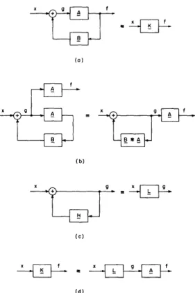
Example 1 was for a feed-through system. Therefore, obtaining its functional expan-sion was a straightforward procedure. We shall now develop the procedure for deter-mining the functional expansion for a feedback system. The single -loop feedback system is shown in Fig. 14a, in which A and B are nonlinear systems that have a known func-tional expansion. Figure 14b is an equivalent system, in which the feedback system of Fig. 14a has been split into the system A cascaded with a simpler feedback system.

+ A (0) X g f B *A (b) (c) f f (d)

Fig. 14. (a) Nonlinear feedback system. (b) Equivalent system. (c) System L. (d) Combination of A and L.

Let B * A = H, and let the simpler feedback system be denoted explicitly by L, as shown in Fig. 14c. Then the feedback system of Fig. 14a, which is explicitly denoted by K, is given by

K = A * L (65)

as shown in Fig. 14d. Since A is known, K can be obtained from Eq. 65, once L has been determined. We shall determine L first and then find K from Eq. 65, because this is easier than developing K directly. (In many problems K can be found directly. In this general case, such a procedure is difficult.)

For the feedback system L, output g is related to input x by

23

--g = x + H[--g] (66) which relates g implicitly to x. However, it is desired to have an explicit relation

g = L[x] (67)

and so, if we substitute Eq. 67 in Eq. 66, we have L[x] = x + H[L[x]]

Writing this as a system equation, we obtain

L = I + H* L (68)

where I is the identity system. Equation 68 is an implicit equation for L. Now, we have assumed that A = A + A2 + +A + . and B = B1 + B2 + + B + .... Therefore

the expansion

H=H = H1 +... +H +... (69)

is known, since H = B * A.

Now, we desire to find L in the series

L=L +L + ... +L +... (70)

Therefore, Eqs. 69 and 70 are substituted in the system equation (Eq. 68), and

L + L + L + ... = I+ (H1+_H2+H3+...) * (L+L 2+L+3+...) (71)

Now the L can be found in terms of the H by equating the nt h-order system on the

-n -n

left-hand side of Eq. 71 to the n -order system on the right-hand side. So that the order can be recognized, Eq. 71 must be expanded as follows:

L1 + L + + ... =I+ (H*L+H*L +H *L 3+...)

+ (H2o(L2) +2H O(L1-L2)+H2 (o) + .)

+ (H3°(L 3) o(LZ.L) +3H+3H3 (L1 2 )

+ H3°(L2+ )+...

Equating equal orders then yields:

L1 = I + H * L1 (72) L2 = H * L + H 2 ) ((L73) 3_{3 nd on.}= 1 *L 3₃ + H2 (L1 .L) + H3 (L3 (74) 2 3 and so on. 24

By way of explanation, if y = A[x] and z = -y, then z = -A[x]. Now, if g = B[x], then f = g + z = B[x] + (-A[x]). Taking f = H[x] = B[x] + (-A[x]) gives a system equation

H=B+(-A) or H = B-A

This defines the minus sign in this algebra. The minus, or subtraction, operation obeys all the rules for the addition operation. Thus by subtracting H1 * L1 from both sides of

Eq. 72, we have L₁ - (H1*L1) = I + (H1*L1 ) - (H1*L1 ) or L1 - (HI*L1 ) =I or (I-Hi) * L = I (75)

because I* L1 = L1. Equation 75 is, then, an alternative form of Eq. 72. In a similar

manner, Eq. 73 becomes

(I-H 1) * L2 - H2 0 (L 2) (76)

and Eq. 74 becomes

(I-H1

)

Now, if we precascade Eq. 75 (formal justification will be given in Sec. VI) by the inverse of (I-H1), which is denoted (I-H1)-1, then

(I-H1 1 *(I-H L1 = (I-H1) (78)

But (I-H 1)-I is the inverse of (I-Hi), and so (I-H1)I * (I-H1) = I, and Eq. 78 becomes

L1 = (H - ) 1 (79)

(If y = _H[x], then there is a K for which x = K[y]. This K is the inverse of H and we shall denote K by H- 1 . The inverse is considered in more detail in sec. 6. 3. The inverse of a linear system is well defined in linear theory.)

Similarly, Eq. 76 becomes

L (IH ) *(H o(L2))

and Eq. 77 becomes

L3 = (I-H1)-' * (2H2o(L1 L2)+H3o(L3))

In this manner, the L can be found for the feedback system L. The functional series for the feedback system K is then given by The functional series for the feedback system K is then given by

Z5

K =A *L = (Al+A 2+...) * (L +L+...) A1 *L + 2 (2) + ZA2 ° (L1 L2

)

A

and so on. The validity of the series expansion

K=K _{- -1} 1 + K + ... _- +K _-n + ... (83)

will be considered in Section VI, but it may be said now that it is generally rapidly con-vergent for sufficiently bounded input.

In any particular problem there are two alternatives. We could use the equations for K for the general case of Fig. 14a (the first three equations are Eqs. 80, 81, and

-n

82), and substitute the particular A and B that are being used. A better procedure is

Fig. 15. Nonlinear servo system.

to work out the Kn, by the method just described, for each particular case. This is not

too difficult after some practice.

As an example of this method, consider the feedback system of Fig. 15. In this case

L = H1 * N * (I-L) (84)

where H1 is a linear system, and N = I + N3 .

This system is sufficiently simple that the series for L can be obtained directly. Equation 84 can be rewritten as

L = H1 * (I-L) + n3H1 * (I-L)3

and substitution of the series L = L1₁ L_-2 + 2 + L₃ 3 + ... _' in this expression yields_{nths3pesinyed}

26

1 -2 -3 1 (-L1-L2-L3-. ) + n3H 1 * (I-L 1-L-L3- ) = (H1*(I-L 1)-H 1*L -H *L3 -... ) +(n ₃H_₁*(I-L 1)3+3n3H1* ((I-L) L2) +...) (85) Therefore L1 =H 1 (I-L) (86) L = -H * L (87) -2 -1 -2 L3 -H1 L3 + n3H * (IL (88)

Rearranging Eq. 86 (in a manner similar to the rearrangement that gave Eq. 79 from Eq. 72) yields

L1 = (I+H1)-I * H

Equation 87 is satisfied for L2 = 0, and this is the only solution (see sec. 6. 3). Rear-rangement of Eq. 88 gives

1 3 3

L3 n3(I+H1)- * H1 * (-L 1) = n3L1 *

(-L

Continuing this procedure gives L4, L5, and so on. In particular, it can be shown that

L4 = 0

L5 = 3n3LI *((I-L 1)2 L3)

L = 0 -6

L7 =n 3L1 * (3(I-L1)L 3 ) + ((I L1)2 L5 )

2. 9 IMPULSE RESPONSES AND TRANSFORMS

It has been shown how the algebra of systems can be used to combine systems. But before the output of a system so described can be obtained for some given input, this algebra must be related to the system impulse responses and transforms. We shall give the relation between the algebraic terms and the corresponding impulse responses and transforms.

By means of this algebra, a system L is expanded in a series L = L1 L2 + +

L + ... , where the L are given in terms of the system's component subsystems.

-n t-n

For an n -order term of the form L = A + B or Ln[X] = A[x] + Bnx] the

corre--n -n n n -- -n -n

sponding functional equation is

27

..

f

n

n)

...

J/ J

+

...

b n(

...

)

Hence, for the algebraic term Ln, where L = A + Bni the corresponding impulse_{-n n -n n'}

response is

in(tl, . .. tn) = an(tl . Itn) + bn(t1l -t )n

The corresponding transform relation is

L (s 1 .. . Sn) = An(S, 1 .'Sn) + Bn(S, ... Sn)

Similarly, it can be shown that for the simple multiplication combination, with L n+m = An Bm, the corresponding impulse response is

1 n+(tl ... t n+m) = an(t₁ ... *tn) bm(tn+l' .. n+m ) (89)

The corresponding transform is

L n+m(sl, . n+m) = An(S1, * * Sn) Bm(Sn+ 'S n+m) (90)

For the cascade situation, with L = A * Bn, the impulse response is

-n -1 n

n (ti . tn) = al(T) bn(tl T, t2 -T, tn-T) dT (91)

and the transform is

Ln( 1 ... Sn) = A1(S 1+S2+... +Sn) Bn(S 1 ... Sn) (92)

The more general cascade operation also has a relation with a corresponding impulse response and transform. If

L =A (Bp.C...'P ) (93)

Lp+g+... +r -= An -- -q -r then

P1q+. .+

-I

...

XCq(tp+l-T .. tp+q - t. T) ... d .. d (94)

and

Lp+q+...+r Sl**Sp+q+... +r) = An(S1+... +Sp Sp+l +...+Sp+q' ... )

X Bp(S1 .... Sp) Cq(SPp+ '...' p+q) (95)

Some of these combined forms, as written, are not symmetrical, but they can be symmetrized, if it is desired. As we have stated, the impulse response h2(t1, t2) can

be symmetrized by forming h2(tl' t2) + h2(t2, tl)

2 (96)

The transform H2(s1, s2) can be symmetrized by forming

H2(sl, S2) + H2(s2, S1)

2

Similarly, for H3(s1', s2' s3) we can construct

6{H 3 ( s l s2' s3)+H3(s1' s3, s2)+H3(s2 s2, s1)+H 3(s2, s3 S1

+H3(s3, s, s 2)+H3(s3, s2, s )} (98)

In general, for Hn(s 1 .. . sn), we add up the Hn with all possible arrangements of

s1, ... , sn and divide by the number of arrangements.

Two examples of obtaining the transforms from this algebra will be given. For the feed-through system L (see Sec. VI):

L = -L1 + L3 (99)

L1 nlAl * B1 (100)

3 L3 = n3A1 B(101)

Let A1 have a transform, Al(s), and B1 have a transform, B (s). We want to find

Ll(s), the transform of L1, and L3(s 1, s2, 3), the transform of L3. By application

2

of Eqs. 89-98, we have L (s) = nlAl(s) B(s). From Eq. 90, B1 has a transform,

3 2

Bl(Sl) B1(s2), and B1 = 1 B1 has a transform, B(sl) Bi(sZ) Bl(s). Equation 92 then

shows that

L3(S1 , S 2' 3) = n3Al(S1 +s+S 2 3) Bl(S1) B1(S2) B1(S3)

29

-The second system is an example of a feedback system (see sec. 2. 8), with

L1 = (I+H1)-1 * H1 (102)

L3 = nL * (I-L1)3 (103)

L_5 3n3L1 * ((I-L 1) .L3) (104)

Let H1 have a transform, H(s ) = A/(s+a), where A >> a. Then (I+H1) has a transform

+ A s +A

s + a s+ a

and, from linear theory, we know that (I+H1)-1 has a transform

1 s+a

1 +H(S ) s+A

Then, from Eq. 92, L1 has a transform

L (S) Ss s a s+A (105)

Since (I-L1) has a transform I - Ll(s) s/(s+A), (I-L 1)2 has a transform

S1 S2

+ A s2 + A

from Eq. 90, and (I-L1)3 has a transform

1 S2

53

1 + A s + A 3 +A

Therefore, application of Eq. 92 to Eq. 103 shows that L3 has a transform

n3A s1 s2 s3

L3(S 2 s3 s +S2 + +A s +A s + A 3A (106)

Also, since (I-L1)2 L3 has a transform

s1 2s

+ A s +A L3(s3'4',s 5)

L5 (Eq. 104) has a transform

3n3A s 1 S

L(S 1, 5 ) +A + L3(s3, s4 s5) (107)

S1 + S5 + s +A +A

With some experience the transforms can be readily obtained by inspection from the algebraic equations. We are still not in a position to use these transforms to compute

30

the system output for a given input. However, at the end of Section III, these trans-forms will be used for this purpose.

2. 10 SUMMARY

We have been concerned with expressing nonlinear systems in terms of their linear subsystems and nonlinear no-memory subsystems. The main tool for combining sys-tems has been an algebra of syssys-tems. The algebraic manipulations required for system combination obey laws similar to those of other algebras. If the algebra of systems were not used, system combination would have to proceed with involved formulas and by a series of clumsy steps. Our algebraic notation consists of a system representation in which only those aspects of the functional representation that are involved in system combination are emphasized. This algebra applies the powerful concepts of operator mathematics to nonlinear systems.

The relation between the algebraic representation and the system impulse responses and transforms has been shown. Particular emphasis has been placed on the transforms in the two examples presented.

31

III. SYSTEM TRANSFORMS

3. 1 INTRODUCTION

We have represented a nonlinear system in terms of its impulse responses hn(tl ... tn), or the transforms Hn(s₁ ... Sn). The system output, f(t), is given by Eqs. 2 and 3. The problem, now, is to obtain the fn(t), and thereby the system output, f(t).

In Section I multidimensional transforms were introduced, and we found that the value of these transforms - just as in the linear case - lies in their making it possible

Fig. 16. Illustrative feed-through system.

to substitute multiplications for convolutions. Not only is this true in calculating the system output, but also in cascading systems. This is shown by Eqs. 91 and 92, and by Eqs. 94 and 95.

Another reason for using transforms is that the form of the impulse responses, even for simple systems, is rather complicated. For example, consider the system of Fig. 16. In this case,

L = L2 = B₁ N2 * A₁

and A1 has a transform A/(s+a), B1 has a transform B/(s+p), and n2 = 1. Therefore,

from Eqs. 90 and 92, L₂ has a transform A2B

L (s1,s 2) = AB (108)

(s 1+s2+)(s 1+a)(s+ )

Reference to Eqs. 89 and 91 shows that the impulse response is

12(tl ,t ₂ ) =2 Be-iT Aae exp-) dT

for t, t2 a 0, since A/(s+a) has an inverse, A exp(-at), and B/(s+p) has an inverse,

B exp(-pt). The form of the limit follows because A₁ and B1 are realizable systems,

and T is integrated from 0 to t or t₂, whichever is smaller. Working out the integral gives

( BA 2 )-at I -at2 -(P -a)t I -at 2

12(t , t 2 )= p-2 a e -e e

for t t >O0 and t < t₂ and

32

12(tt 2) =(3A2 )(eatl eat2 -e atl e(Pa)t2} (109)

for tl, t2 andt 2 < t. Comparing this result with Eq. 108 shows the simplicity of the

transform, as compared with the impulse response.

Our object, now, is to show how the transforms can be used to determine the output of a system. Emphasis will be placed on an important special case for which the trans-forms are factorizable. This situation arises when a nonlinear system is lumped.

We shall be in a position to apply the functional representation to the solution of nonlinear system problems, and several examples will be given.

3.2 MULTIDIMENSIONAL TRANSFORMS

Higher -order transforms were defined by Eqs. 10 and 11, and a method of using the transforms was indicated. The linear case is well known. If

fl(t)

=

then

F1(s) = H1(s) X(s) (111)

Consider the quadratic system

f2(t) =

f

To use transform theory here, we must artificially introduce a t and a t2, so that

f(2)(t) t₂) =fh(( ' T2) X(tl-T) 1 x(t 2-T2 ) dT2dT2

and then

F(z)(Sl' s2) = H2(S 1' 2) X(s1) X(s2) (113)

Formally, at least, F(2)(S1, s2) could be inverted to give f(2)(tl, t), and when f2(t) is

the desired output, f2(t) = f(2)(t,t). This is illustrated in Fig. 17. We have f2(tl, t2),

which could be plotted by contours on the t, t2 plane, but we are only interested in

f2(tl,t 2) along the 45° line where t1 = t2 = t. This method generalizes to higher-order

cases. For example,

f(3)(tl'tz't3)

=f

but the quantity of interest is f3(t), with

f3(t) = f(3)(t, t, t) (114)

The procedure of taking a number of variables t, ... tn as equal will be called

"associating" the variables. The procedure that has been outlined is not particularly

t2

Fig. 17. (t, t 2) plane showing t1 = t2 line.

practical, since it involves taking an n-dimensional inverse transform. A better pro-cedure is to associate the time variables in the transform or frequency domain. That is, given F(2)(sl, S2) as the transform of f(2)(t1l t2), then F2(s), the transform of f2(t), will

be found directly from F2(S1 , s2). The formal relation is

Fz(S) = j - +jo F(2)(s-u,u) du (115)

where is a suitably chosen real number. A proof is given in Appendix A. 2. This relation is similar to the Real Multiplication Theorem of linear theory (9). For higher-order transforms, Eq. 115 can be applied successively to associate the variables, two at a time. Then, for example, for F(3)(s1 , s2, s3),

F

(s)

=(-j)2

-jo

I1

F(

)(s-u

,

This is still not very practical because convolutions must be made inrthe transform domain. The great value of making the associations in the transform domain lies in the fact that these associations can be made by inspection in a large class of problems. This class is the nonlinear generalization of the linear situation in which the transforms are factorizable. The constraint on the system is that it be lumped - that is, that all the transforms of the linear subsystems be factorizable.

Then for the system H, where H = H + H + ... + H + .. , we have

N P. M

H1(S) i= + i R.s (117)

i=l pii=0O

where Pi, Pi, and Ri are complex constants. This is familiar from linear theory, and note

that terms of the form Pi/(s+Pi)n, for n > 1, have been left out. Such terms will be con-sidered separately. If X(s) is the transform of the input to H, then the transform of the

output from the linear portion H1 is given by Fl(s) = H1(s) X(s). If Y(s) is factorizable,

then it is known from linear theory that Fi(s) has the same form as Eq. 117, if multiple-order poles are neglected. In the class of systems that is being studied (linear subsys-tems with memory and nonlinear no-memory subsyssubsys-tems) the most general second-order term is a summation of terms of the form

A1 (B1.C1) (118)

The determination of the transform of such a term was considered in Section II. It is A1(s1+s2) B1(s1) C (S2)

where Al(s), Bl(s), C1() are the transforms of the systems A1, B1, and C1,

respec-tively. If the input has a transform X(s), then the contribution to the system output that is attributable to the output from the term of Eq. 118 has a second-order transform

Al(s1 +s2) B1(S1 ) Cl(s2) X(sl) X(s2) (119)

If Bl(s), Cl(s), and X(s) are of the same form as Eq. 117, then Bl(sl) X(s₁) and Cl(S2) X(s2) have this form, and Eq. 119 becomes

B. C.

Al(Sl+s2) + 1 (120)

1 2 S + S 2 +

where Bi, Ci,

pi,

M be factorizable, but it will generally be assumed to be so. Note that the terms Rs

i=O have been excluded from the summation of Eq. 120. This is done because these terms are the transforms of impulses, doublets, and so forth, and such functions do not exist when squared. Should these idealizations occur in a physical problem, they must be removed and replaced by the real physical signals.

The inspection technique can now be developed. Consider a typical term in the second-order case (Eq. 120):

G(2)(s, S 2 )=A 1(S1+S) 1 s + s +

Application of the transform-domain association equation (Eq. 115) gives

G2(S) = 2 j

f

du

The term that is to be considered is

1 B C

du

2j -u+ p u +y du (122)

But (B/(sl+p)(C/(s₂+y)) is easily inverted, and has an inverse transform

-Pt 1 -Yt2

Be Ce tl' t2 0

Setting t = t₂ = t gives

B Ce- (P+Y)t t > 0

This has a transform, BC/[s+(P+y)], and it is seen that

1 B C du= BC (123)

2_{irj s-u + u s+(P+Y)}

Finally, we have

G2(s) = A1(s) BC

s + (+y)

where G2(s) is the transform of g2(t); and g2(t) = g(2)(t,t), where g(2)(tl,t2) is the inverse

transform of G(2)(s1 , s2). That is, we have made the association of t and t2 by a

transform-domain manipulation that gives us the ordinary linear transform of the desired time function g2(t). Furthermore, this manipulation can be done by inspection.

That it is an inspection technique is seen by noting that the association of t and t2

changes

(2)(Sl, S2) = A(Sl+S) B C (124)

into

G2(s) = A(S) BC (125)

s + (1+y)

Examination of Eqs. 124 and 125 shows that the change is a very obvious one and can be obtained by inspection.

Higher-order transforms can be reduced by applying the inspection procedure to associate the variables, two at a time. For example, consider the third-order term

A B C C C (126)

Sl +s2 + 53 + a s3 2 + + P S1 + Y 2 + Y S3 + Y

Application of the formal association equation (Eq. 115) to associate s2 and s3 yields