Cosmological signatures in galaxy cluster structures

Cosmological Signatures in Galaxy Cluster

Structures

by

James J. Frederic

Submitted to the Department of Physics

in partial fulfillment of the requirements for the degree of

Doctor of Philosophy

at the

MASSACHUSETTS INSTITUTE OF TECHNOLOGY

January

1997

@

Massachusetts Institute of Technology 1997. All rights reserved.

A uthor ... ..

....

..

...

Department of Physics

January 13, 1997

C ertified by .. '. .

-

... ...

...

...

Edmund Bertschinger

Associate Professor

Thesis Supervisor

A ccepted by ...

...-...

George F. Koster

Chairman, Graduate Committee

FEB 12 1997

Cosmological Signatures in Galaxy Cluster Structures

by

James J. Frederic

Submitted to the Department of Physics on January 13, 1997, in partial fulfillment of the

requirements for the degree of Doctor of Philosophy

Abstract

We study substructure in X-ray clusters of galaxies by application of a set of statistics, the power ratios of Buote & Tsai (1995), to a simulated cluster and in the context of a simple analytic model for merger events. The simulation involves a newly de-veloped code for performing high resolution gravity and gas dynamics simulations in cosmological volumes.

Thesis Supervisor: Edmund Bertschinger Title: Associate Professor

Acknowledgments

I am grateful to my advisor, Ed Bertschinger, for all his support: scientific, profes-sional, financial, and even moral. Ed's encouragement and confidence in my ability provided me a needed and much appreciated pick me up on many occasions.

As I finally leave the role of student, formally at least, I wish to thank my parents, Wayne and Rosemary Frederic, for putting me on this path and encouraging me along it. As a parent myself now I realize more each day the sacrifices they made to make me who I am. Each night when I return from work (too late), my frustrations melt away in the excited greeting of my young son Ethan. My greatest hope for my relationship with him is that when he is a man he is still as happy to see me as I am to see my parents.

All the long days, nights and weekends that went into this thesis place me deep in

debt to my wife Tonya. Tonya, I.O.U. one year of parenting. Thanks for shouldering more than your share of the home burdens while I worked, for being a great mother to Ethan, for all your love.

Thanks to Ethan, my little buddy. Without understanding how or why, you make any burden tolerable, and you make me happy.

And to the next little Frederic, due any minute now, thanks for waiting. Daddy's ready now.

Contents

4.2 Cluster evolution in power ratio space . ... 25

4.3 Substructure survival time . ... ... 29

5 An analytic model for predicting power ratios 37 5.1 Merger rate ... .. . . ... ... . 38

5.2 Infall model ... ... 43

5.3 Power ratio prediction ... ... 49

5.4 Testing the predictions ... ... ... 52

6 Conclusions 64 A Computational details 68 A.1 Initial Conditions ... ... 68

Chapter 1

Introduction

There are many ways in which galaxy clusters may reflect cosmological parameters. For example, the normalization and shape of the cluster luminosity function certainly reflect the amplitude and shape of the power spectrum of initial density fluctuations. Assuming that the ratio of baryonic to total mass in large clusters is the universal ratio, measured baryon fractions can be combined with nucleosynthesis constraints on the overall baryon density to infer the total mass density Q (White et al. 1993). Measurement of the Sunyaev-Zel'dovich effect in clusters can be used to determine the cluster's true size and hence its distance, bypassing the many rungs in the cosmological distance ladder and allowing determination of the Hubble parameter H0.

The internal structure of clusters of galaxies may be a powerful discriminator of cosmological models as well. In particular, the amount of substructure in clusters is expected to be highly sensitive to the mean density of the universe (Richstone et al. 1992). Assuming that mergers and accretions onto clusters impart internal structure to the clusters and that such structure is then erased via relaxation processes, the amount of substructure surviving today is a measure of the epoch of cluster formation. More substructure indicates more recent cluster formation and a higher mean matter density. This approach has been taken theoretically by Richstone et al. (1992), Lacey & Cole (1993, 1994), and Kaufmann & White (1993). Each of these authors applied extensions of the Press & Schechter (1974) formalism to study the fraction of clusters which have recently formed. By assuming some value for the survival time

of substructure, and by estimating the fraction of clusters which currently possess substructure, Richstone et al. (1992) and Lacey & Cole (1993) determined that the frequency of substructure present in available data favors a large value for the mean mass density of the universe, Q > 0.5. Kauffmann & White (1993) reached no conclusion in this regard, as the survival time of substructure is so uncertain. Other cosmological parameters, such as the power spectrum and cosmological constant, may also leave a measurable signature in cluster structures (Richstone et al. 1992, Lacey & Cole 1993).

The issue of substructure survival time lends itself naturally to testing by simu-lation. Nakamura et al. (1995) and McGlynn & Fabian (1984) have addressed this issue directly, albeit with simple models of equal mass subclusters, without gas, and not in a cosmological setting. Taking the substructure survival time to be the time from the initial encounter until only a single density peak remains, they find that this timescale is very sensitive to the assumed mass profiles and velocity dispersions of the subclusters, as well as the initial conditions for the orbit. Other simulators, including Crone et al. (1994), Evrard et al. (1993), Mohr et al. (1995), Buote & Tsai (1995), and Buote & Xu (1996) have taken a different approach: simulating clusters in differ-ent cosmological models in order to establish the model discriminating power of their structure statistics. In addition, Mohr et al. (1993, 1995) compared the substructure measured in the simulated clusters to that in data from the Einstein observatory, while Buote & Tsai (1996) and Tsai & Buote (1996) made similar comparisons to ROSAT data. The results of Mohr et al. favor a high density universe, Q = 1. Buote & Xu (1996) reach the opposite conclusion. We discuss possible sources of this dis-crepancy in Chapter 4, and by comparison to our simulation identify a small bias in the results of Buote & Xu.

In order to be interpreted these effects should be calibrated using simulations. Unfortunately, the X-ray luminosities of clusters, being proportional to the square of the electron density, are dominated by the dense cluster cores. Accurately simulat-ing these cores requires extremely high resolution and correspondsimulat-ing computational resources. The radiative cooling of the plasma must be included in simulations of

the largest clusters, where cooling flows may increase the central densities. Using simulations to calibrate cluster baryonic mass estimates and measurements of the Sunyaev-Zel'dovich effect also requires resolution of cluster cores.

Extracting cosmological information from cluster structure requires that substruc-ture be quantified. Unfortunately, some measures of substrucsubstruc-ture in the X-ray images of clusters have also been most sensitive to cluster cores (Mohr et al. 1993, Evrard et al. 1993). However, Buote & Tsai (1995) have proposed a substructure statistic based on the power in multipole moments of the projected gravitational potential. Their so-called "power ratios" are most sensitive to structure outside the cluster cores. With this statistic substructure can be quantified in simulated clusters without the need for ultra-high resolution cores and cooling. Once substructure statistics have been established, we can study substructure survival time, the expected distribution of substructure statistics, and the evolutionary history of clusters measured in the space of the substructure parameters.

Another advantage of the power ratio statistics for quantifying substructure is that they are most sensitive during the earliest stage of the merger, as the subclump falls toward the main cluster. In effect, as viewed via power ratios, the merger ends before the complex dynamical processes of gas relaxing to hydrostatic equilibrium take place in the core. This is advantageous both for simulations, as the modelling of these processes is less important, and for making models to describe the merger events themselves. In Chapter 5 we fashion such a model by combining the merger rate, based on the Press & Schechter (1974) formalism, with a simple model describing the infall of a subclump onto the main cluster.

In order to simulate clusters for study I have developed a new code, combining an adaptive N-body code for evolving collisionless dark matter and a fixed resolution hydrodynamics code for evolving collisional gas. Grid based Eulerian gas codes have been used in engineering and scientific applications for many years and have been well studied (Ryu et al. 1993, Bryan et al. 1995). They are limited, however, by finite computational resources. Accurate cluster simulation requires that the mass field in a large computational volume be computed, and high spatial resolution requires a

prohibitively large computational grid. Lagrangian approaches make more efficient use of computational resources by allowing spatial resolution to flow to where it is most needed. Smooth Particle Hydrodynamics (SPH), for example, uses particles as elements of both mass and force resolution. This technique excels in high density regions but does a poor job in low density regions where particles are few. Moving grid techniques developed recently (Gnedin 1995, Pen 1995) also concentrate compu-tational effort, but can have problems in regions where the flow is highly deformed. Finally, Eulerian techniques which employ adaptively nested levels of resolution are being implemented presently and are very promising as they are, conceptually at least, only marginally more complicated than the single grid methods on which they are based (Bryan 1996). While all these methods are useful, the single fixed grid Eulerian methods are the simplest and best understood. One of these, the Piecewise Parabolic Method (PPM) (Colella & Woodward 1984) as implemented in the KRONOS code (Bryan et al. 1995), is the basis for the hydrodynamic portion of my code, described in Chapter 2.

As described above, the combination of a fixed, high resolution grid and a large spatial volume can be satisfied only at high computational cost. I have therefore bor-rowed from the Lagrangian philosophy the idea of solving the relevant equations only where the computational effort is most fruitful. Specifically, the accurate simulation of a cluster requires evolving the mass field in a large volume around the cluster be-cause gravity is a long range force. The equations of gasdynamics, however, are short range, and as such need only be solved in a much smaller volume around the cluster. I have therefore developed a code which evolves the mass and gravity fields in a large volume and the gas density, velocity and energy fields in smaller, embedded volume. The Poisson equation and Euler's equations each require that boundary conditions be prescribed. The usual procedure for cosmological simulations is that periodic boundary conditions be applied. This can still be done for the mass and gravity fields. Since the gas is only explicitly evolved in a subvolume of the total simulation, its boundary conditions must be handled differently. The total mass field is represented by dark matter particles in most of the volume, and by dark matter particles and the

gas density field in the gas subvolume. Therefore the gas is assumed to follow the dark matter outside the gas subvolume. At the edge of the gas subvolume, boundary conditions for the gas can be estimated from the dark matter. Determining the total mass and velocity fields from the particle distribution is straightforward. The gas can be assumed to have identical velocity and density in proportion to the mean gas mass to total mass ratio. The gas evolves adiabatically until shocks form, and since the main shocks in a cluster's formation begin at the cluster center and propagate outward, the gas energy, temperature and pressure at the boundary can be assigned assuming the gas entropy is still primordial.

In chapter 2 we present a description of the simulation code, with additional details given in the appendix. Chapter 3 describes the cosmological model we simulate. Chapter 4 presents statistics for measuring substructure and its survival time and analyzes the simulation in light of those statistics. In Chapter 5 we present a model for determining the dependence of the power ratios on cosmological parameters. Chapter 6 presents conclusions.

Chapter 2

The Code

The simulations were performed using a hybrid code constructed from two well tested codes, the P3M2 code of Bertschinger & Gelb (1991) and the KRONOS code of Bryan et al. (1995). The combined code is called P8M31.

The P3M2 code solves the equations of Newtonian gravity and dynamics for a sys-tem of collisionless particles in a Friedmann-Robertson-Walker cosmology. Comoving spatial coordinates x are used, and the time coordinate - (not conformal time) is related to proper time t by dT = dt/a2, where a is the expansion factor which relates

proper distance (r) to comoving distance (x) by dr = adx. In these coordinates, with

a = 1 corresponding to the present, Poisson's equation becomes

V20 = 47rGa2p6, (2.1)

where G is Newton's gravitational constant, p is the mean proper mass density, 6 =

p/p - 1 is the overdensity, and q is related to the Newtonian gravitational potential

4 by ¢ = 4 - 27rGa2px2 2/3. The equation of motion for the collisionless dark matter

particles is

d2

dT

a

,

(2.2)

1_{P3M stands for Particle-Particle-Particle-Mesh and is more properly written P}3_{M. P3M2} uti-lizes an extra, adaptive layer of refinement with a finer scale P3M calculation, hence it is more properly written (p3M)2. The KRONOS code uses the Piecewise Parabolic Method, or PPM. Com-bining powers, (p3M)2.ppM = p8M3.

where g = -VO is the gravitational acceleration.

The equation of motion for the particles is integrated by the second order accurate leapfrog technique,

yn+1/2 = + ?nAtn

/2

vn+l = + r+1/2Atn (2.3)

Yn+1 = +1/2 + %+l1At/2,

where the superscript n is the timestep index.

The Poisson equation is solved approximately in several steps. First, long range forces are calculated by the particle-mesh (PM) technique. In regions of low particle density a short range correction is applied to each pair force in a direct sum over pairs of near neighbors. Together, these two steps are called particle-particle - particle-mesh, or P3M (Hockney & Eastwood 1981). In regions of high particle density, the computational cost of direct pair summation can be prohibitive. Here an adaptive technique is used in which a fine grid is used to perform a second level PM calculation, followed by a further pair summation over only very near neighbors. The short-range (PP) correction to the long-range (PM) force is designed to produce a net pairwise force given by a Plummer law, F = Gmlim2 (ri - r)/[(5i )2 + 2]3/2, which weakens

at short range to minimize two-body relaxation and to maintain the accuracy of the time integration.

The KRONOS code solves Euler's equations of inviscid, compressible fluid flow, while also solving the Poisson equation and integrating the trajectories of dark matter particles. The KRONOS gravity solver uses the strightforward PM technique, but in the combined code P3M2 performs the gravity calculation and leaves KRONOS to handle the gas dynamics only. The equations governing the gas evolution are

0

0

-tPb + PbV' = 0, (2.4)

-pbv + (pbvizvj + P6ij) pbg' , (2.5)

atE + Ori (E + P)vi = pbvJgj, (2.6)

where Pb is the baryonic (gas) proper density, Vi is the proper velocity, P is the gas pressure, E is the total gas energy density, and ' is the gravitational acceleration vector. Cosmological flows often occur in which high bulk flow velocities cause the total gas energy to be dominated by the kinetic energy, so that small relative errors in the total energy integration can yield very large temperature errors. In order to accurately integrate the gas temperature (or equivalently the internal energy or pressure) KRONOS also integrates the following equation for the gas internal energy density e:

e + evi= P 2v . (2.7)

Ot Orz dri

Like P3M2 the KRONOS code also uses a comoving coordinate system, but with different time, mass, velocity, energy and gravity variables. The combined P8M3 code calculates conversion factors for these quantities.

The gas equations are integrated numerically by the Piecewise Parabolic Method (PPM), a third order accurate, grid-based technique in which the cell-averaged gas variables (density, velocity and energy) are represented on a grid and the three di-mensional fluid equations are solved as a series of one didi-mensional problems. PPM is one of a general class of higher order Godunov methods which employ a Riemann solver to calculate mass, momentum and energy fluxes through cell faces. PPM can resolve shocks in one or two grid spacings. Good descriptions of the method are given in (Colella & Woodward 1984, Bryan et al. 1995).

Two versions of the combined P8M3 code have been written; one for serial and shared memory parallel machines and another which uses message passing for a dis-tributed memory parallel computer. Some of the technical aspects of these two im-plementations are different, and will be described below.

Combining the P3M2 and KRONOS codes required changes to the treatment of gravity by the gas code as well as establishing communication between the two algorithms. As originally written, KRONOS used a simple PM gravity solver which produced the gravitational potential on the gas grid. This potential was differenced

wherever the gravitational force was needed. The P3M2 code produces more accurate gravitational forces directly, with no differencing of potential, by using four Fourier

transforms (p --+ , gi -- gi) instead of two (p --+ , q -- q). Therefore instances

of potential differencing in the KRONOS portion of the combined P8M3 code were changed to use the P3M2 force directly. The P3M2 gravity solver also utilizes a high order interpolation function, TSC (Triangular Shaped Cloud) (Hockney & Eastwood 1981) and an optimized, anti-aliased Green's function, as opposed to the lower order CIC (Cloud In Cell) (Hockney & Eastwood 1981) interpolant and simple Green's function of KRONOS.

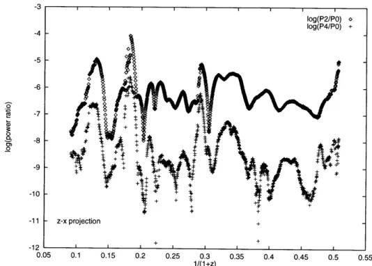
The necessary communication between the gravity and gas portions of the code was implemented differently in the shared and distributed memory versions of the program. The shared memory code adopts the basic structure of KRONOS, with calls to P3M2 routines where necessary. The distributed memory code is based on the P3M2 code, with calls to KRONOS routines. In each, when calculating the density field or gravity, each gas cell is treated as a "particle" with the appropriate mass. This is accomplished in the shared memory code by adding a loop over gas cells wherever there was a loop over dark matter particles in the gravity routines. For example, the original P3M2 code contains a loop over particles in which the mass of each particle is interpolated onto the density grid in preparation for the PM force calculation. The combined code adds a loop over gas cells and treats each of those cells as a "particle" with mass equal to the gas density times the volume of the gas cell.

In the original distributed memory P3M2 code, each processor maintains a list of particles which reside in a particular volume. To account for the gas in the combined code, these particle lists are expanded to include gas "particles." Hence the gas has two representations, one as a grid of density, velocity and energy, and another as "particles" with mass and velocity. The former representation is used by KRONOS, the latter by P3M2. These two representations must, of course, be kept consistent. For this purpose special routines were written to send portions of the gas grid, which is maintained on a single processor, to the processors whose assigned spatial volumes

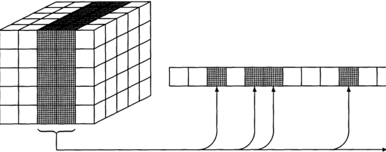
overlap the gas volume. These processors then use the gas density and velocity to update the masses and velocities of the gas "particles" contained in their particle lists. This procedure is shown schematically in Figure A.2. On the left is a representation of a 53 _{grid of gas data (e.g., density), which resides physically on processor 0. On}

the right is a particle list (e.g., mass) which resides physically on, say, processor 5. The two shaded slabs of the gas grid in this example lie within the portion of the simulation volume assigned to processor 5. Hence, for each of these shaded gas cells the processor 5 mass list has an entry. A separate list of particle indices stores a global integer tag for each particle, for which there is a one to one correspondence between the tag of a gas "particle" and it's location in the gas grid. A similar procedure is used to send the calculated gravity at each gas "particle" back to the gas grid.

The basic code structure for the distributed memory version of the code is repre-sented in Figure A.2. This shows that at the beginning of each timestep, gas density and velocity are sent from the gas grid to the particle lists. The gas density is used in the construction of the total density field needed for the PM force calculation. The leapfrog integration scheme (Eqn. 2.3) for the dark matter trajectories and the Riemann solver used by KRONOS require the density field to be evaluated one half timestep ahead of the current time. For the dark matter particles this is easily ac-complished by integrating their positions forward one half step before performing the force calculation. To approximate the gas density at one half timestep ahead, the particle representation of the gas is used, and the gas "particles" are moved off their fixed grid postions by iAt/2. This is why the gas velocity must be passed from the gas grid to the particle lists before the computation of the total density field begins. Note however, that the gas "particles" must be returned to their grid positions after the total density is computed so that the gravitational force felt by each gas "particle" is the force at the grid position at the center of the gas cell.

The gas solver (KRONOS) requires boundary conditions for the gas volume at the beginning of the timestep. As these are determined from the dark matter density and velocity fields, they must be computed before the particle positions are integrated forward the first half timestep. For this calculation, each processor determines which

portion of the gas volume, if any, resides locally, and then uses TSC interpolation to compute the density and momentum density fields at the boundary cells of the gas volume. Dividing the latter by the former gives the velocity field at these points. The density and velocity boundary values are then passed from the particle list structure on each processor to the gas grid structure on processor 0.

Next, the particle postions are integrated forward one half timestep and the gravity calculation commences, modified only2 _{to move the gas "particles" back to their grid} positions after the total density is calculated, as described above. Then the particle velocities are updated by one full timestep and the positions by the second half timestep.

After the gravity calculation, the gravitational acceleration at each gas "particle" must be passed back to a grid structure on processor 0. KRONOS is called next, to update the gas variables by a full timestep, and the next timestep can begin.

20Other modifications to the gravity code were added to minimize memory usage. These, however,

Chapter 3

The Model

We evolve a cosmological model which is consistent with observational constraints (Ostriker & Steinhardt 1995, Liddle 1996, Kochanek 1996).

Ho = 100h km s-1 Mpc- ' = 75 km s-'Mpc-1 (3.1)

QCDM + QB -QA = 1 (3.2)

-B = 0.015h- 2 _{= 0.0267 (3.3)}

QCDM + QB = 0.3. (3.4)

Within this cosmological context we simulate a 51.2 Mpc comoving volume with the dark matter density field sampled using 6069442 particles with nested mass reso-lution. The innermost 16 Mpc cube contains particles with a mean spacing of 100 kpc (comoving), corresponding to a mass of 4.7 x 107M® per particle. This is the total mass of a 100 kpc cube at mean density, including dark matter and baryons (gas). When dark matter particles fall into the gas-filled volume their mass is scaled down

by QCDM/(QCDM + QB). A layer 4 Mpc thick holds particles with twice the spacing

and eight times the mass of the central cube. Two more layers of 6.4 Mpc and 7.2 Mpc each have a further coarsening of the mass resolution by the same factors over their inner neighbor. The largest particles then have masses of 2.4 x 1010_M

0 and reside at least 18.4 Mpc from the center of the simulation volume. These distant,

massive particles provide the tidal forces under which the cluster will evolve.

The central 10 Mpc (comoving) volume also contains a grid of 100' gas cells. The mean gas mass per cell is 4.2 x 106_M®.

Initial conditions are generated using the COSMICS package of Bertschinger

(1995) First, the linearized Einstein and Boltzmann equations are integrated to

com-pute the matter transfer function. An initial Harrison-Zel'dovich spectrum P(k) oc k is assumed. The resulting transfer function is used to generated a constrained random realization of initial conditions. The constraint applied is that the central overdensity, when smoothed under a Gaussian of width 6.4 Mpc, would have a value of 0.7, or

2.5a, where a is the root mean square value of the smoothed overdensity. The 6.4

Mpc Gaussian encloses the same mass as a 10 Mpc top hat, or 2.0 x 1014_M

0, which is a medium sized cluster. Other simulators (Frenk et al. in progress) have used constrained initial conditions to generate unreasonably large clusters, with the result that the cluster evolution was affected when the nonlinear scale approached the size of the simulation volume. Here we have been careful to chose a perturbation which will result in a good size cluster while ensuring that such a cluster is not an extremely rare event in a volume of this size. Using the fitting formula for peak number density given by Bardeen et al. (1986), we find that the expected number density of 2.5a peaks in our simulation volume is 0.5.

COSMICS produces a realization of the density and velocity fields (and equiva-lently, the displacement field) of the mass. The central 100 Mpc volumes in these fields are used to generate the initial conditions for the gas. The gas density is set proportional to the total density, the gas velocity is set equal to the particle velocity. The P8M3 code determines the appropriate temperature field by assuming the gas entropy is constant in space. The mean gas temperature is chosen appropriate to the initial simulation redshift.

Initial particle displacements are determined from the linear transfer function by the Zel'dovich approximation. The initial simulation redshift is set by requiring that the maximum displacement be no larger than 100 kpc, the mean interparticle spacing in the high resolution central volume of the simulation. This results in an initial

redshift of zi = 83.

The gravitational force between particle pairs is softened to a Plummer law, for which the potential energy is given as

Gm m2

U=

Gm

(3.5)

with E = _{0.04 Mpc. With this softening, the force between a pair of particles 100 kpc}

apart is 80% of the true (unsoftened) force. In this way the force resolution of the gravity and gas portions of the code are kept consistent at 100 kpc.

Chapter 4

Substructure

Galaxy clusters were first identified optically as regions of high galaxy density pro-jected on the sky. Abell (1958), for example, identified clusters by the number of galaxies projected within a 1.5h- 1 Mpc radius circle. The most obvious property of optical clusters is their richness, which is roughly the number of galaxies. But they also display different morphologies. Abell (1965, 1975) classified his clusters on a sequence from regular to irregular. Zwicky et al. (1961-1968) based their classifica-tions on the relative compactness of the cluster. Bautz & Morgan (1970) devised a classification scheme based on the brightest galaxies in the cluster. Rood & Sastry (1971) developed a system reminiscent of Hubble's "tuning fork" diagram of galaxy types. Morgan (1961) and Oemler (1974) classified clusters by their spiral and el-liptical fractions. These classification systems are highly correlated, indicating that cluster optical morphology can be approximately described by a simple sequence from more to less regular (Sarazin 1988). The "ideal" regular cluster would have spher-ically symmetric distribution in position, and the line-of-sight velocity distribution would be Gaussian, although the velocity dispersion generally decreases with radius from the cluster center (Sarazin 1988).

Irregularity in clusters sometimes manifests itself as multiple peaks in galaxy num-ber density, either projected or in redshift space, indicating that a merger has recently occurred. Geller & Beers (1982) found that 40% of rich clusters have multiple pro-jected density maxima. Dressler & Shectman (1988) made use of velocity information

also and claimed to find significant substructure in 30-40% of clusters. West & Bothun (1990) find "definite substructure" on Mpc scales in 30% of their sample.

Clusters can be imaged with better statistics in X-rays, as there are many more X-ray photons than galaxies available. Forman & Jones (1970) and Jones & Forman (1992) developed a classification system based on structure in the X-ray images. Applying this to images obtained by the Einstein satellite, they identified about 20% of their clusters as "double" or "complex." Mohr et al. (1993, 1995) proposed statistics for quantifying substructure in X-ray images and applied them to Einstein data. By comparing these to simulated clusters (Evrard et al. 1993) these authors conclude that the observations favor a high value for Q.

An alternative to observational (optical and X-ray) identification and classification of clusters is the theoretical definition based on mass. Clusters correspond to the highest density regions of an appropriately averaged mass density field. The mass density of the Universe varies on all scales. In order to isolate the scales relevant to clusters, one first smooths the density field on cluster scales. Define the mass density field p(£) and the overdensity

6(,) = (4.1)

P

where p is the mean density. The density smorothed on mass scale M is then

6(0, M) = 6(:?)W(I£ - i1, M)dx', (4.2)

where the smoothing window function is spherically symmetric about Y and has com-pact support. The mass scale M is related to a length scale Rs by

M = pW(r, M)4wrr2_{dr. (4.3)}

Clusters are then identified with the regions above some threshhold in the smoothed density field. If this field corresponds to the present, then this threshhold density will be around 200 (Lacey & Cole 1993). Because the effects of non-linear gravitational

evolution dictate the spectrum of density fluctuations at present, it is more convenient to work with the initial, linear density field. The statistics of this field are dictated by the cosmological model, and are specified by a power spectrum of density fluctuations which are usually assumed to be Gaussian. The high density regions in this smoothed initial density field are assumed to evolve into galaxy clusters.

This cluster definition, based on the firm mathematical grounds of density fields, power spectra, smoothing functions, etc., is attractive to theorists but not easy to con-nect to observations. It is most useful for predicting things like the mass distribution of clusters as a function of time, something which is not easy to observe.

In practice there are two approaches for studying cluster distributions based on the initial density field. In the peaks method (Bardeen et al. 1986), high peaks in the smoothed initial density field are considered to be the locations of non-linear structures in the evolved field. E.g., the highest 10% of the peaks in a density field smoothed on cluster mass scales correspond to the most massive 10% of clusters. Statistics such as the correlation functions of the peaks are then thought to apply to the corresponding clusters as well. The other approach, pioneered by Gunn & Gott (1972) and Press & Schechter (1974) and extended by Bond et al. (1991) and others, utilizes the analytic solution for the collapse of a spherical overdensity. The power spectrum of fluctuations in the smoothed initial density field determines the distribution of overdense regions. Each of these regions is modelled as a spherical perturbation in an otherwise flat Universe to give both a mass and a collapse time for that mass. This prescription has been used to determine tha mass function of non-linear structures as a function of time (Press & Schecter 1974), as well as the merger rates, formation histories, and survival times of dark matter halos (Lacey & Cole 1993, Kauffmann & White 1993).

This thesis deals with a simulated X-ray cluster and with statistics based on the initial density field. Because the simulation resolution and input physics are not sufficient for modelling individual galaxies within the cluster, galaxy counts or cluster richness are not useful criteria for defining or classifying clusters or for measuring substructure. Instead we opt for the following definition: a cluster is a spatially

isolated high density region which contains hot, diffuse X-ray emitting gas, and which formed from the mass in a high density region of the initial density field.

In order to make a clear definition of substructure within clusters it is useful to define what substructure is not. A substructureless cluster is spherically symmet-ric. Departures from symmetry, then, are indications of substructure. However, we wish to avoid any definition of substructure which divides clusters into substructure "haves" and "have nots," since there is of course continuum of degrees of departure from symmetry. Such a division would be artificial. A better approach is to allow operational definitions of substructure based on quantifiable measures. This way we avoid terms like "significant substructure."

4.1

Substructure Statistics

One attempt at quantifying substructure in X-ray maps of clusters of galaxies is due to Mohr et al. (1993). They develop statistics based on the Fourier transforms of annuli in a circular image aperture. Each annulus of some specified thickness and mean radius f can be decomposed in a Fourier transform

I(0, i) =

Z

m=O

The coefficients An and Bn are then

An f I(0, i) cos(nO)dO, _(4.5)

B - f 1(0, F) sin(nO)dO. _(4.6)

The center of each annulus is not determined a priori, but is instead set to be the position for which the difference between the center and centroid of the annulus is minimized. Specifically, this corresponds to minimizing A2 + B1.

shift is

w_ 2 Nj ' (4.7)

where j is the annulus index, 5j is the annulus centroid position, Nj is the photon count in the annulus, and (7) = E Nj7j

/

Mohr et al. (1993, 1995) also introduce an axial ratio

2

A+

_B22

r7(T) ~ 1- (4.8)

r(dI/dr)

and an ellipsoidal orientation angle

1 _J32

0() = I tan- ( B2) (4.9)

2

A2

as well as averages and variances (over annuli) of each of these. 1

In Evrard et al. (1993) these authors apply these statistics to clusters simulated under different cosmological models and argue that the statistics discriminate well between models of different density, though not between low density models (Q =

0.2) with and without a cosmological constant providing spatial flatness. Mohr et al. (1995) apply these statistics to a sample of Einstein clusters and find that the distributions of centroid shift and axial ratio agree better with their Q = 1 CDM simulations than with their low density simulations.

Another method for quantifying X-ray substructure was proposed recently by Buote & Tsai (1995). Their power ratio statistics are based on the multipole ex-pansion of two dimensional gravitational potential, which solves the two dimensional Poisson equation sourced by the projected mass density E interior to an aperture radius R,

V2_{1F = 27rGE. (4.10)}

1

The multipole expansion is given by

I(R, ¢) = -2Gaoln(1/R) - 2G mRm _{(am cos mq + bm sin m¢) , (4.11)}

m=1 mRm

am(R) = (r, )rm _{cos me rdrd¢, (4.12)}

bm(R) = E(r,)r m _{sin m rdrd¢.}

(4.13)

The power in the mth multipole due to mass interior to R is the azimuthally averaged value of the square of the mth term in equation 4.11,

Pm(R) = f Tm(R, ) Im(R, )do , _(4.14)

which reduces to

4G2

Po = [2Gao ln(R)]2 , Pm>o = 2 (a + b ). (4.15)

2m2R2m m m)

The projected mass density E, while available in principle from weak lensing maps of clusters, is not in practice well determined for any real clusters. Buote & Tsai (1995, 1996) were concerned with the dynamical state of clusters and argued that while this would be best reflected by using the projected mass density E, the X-ray surface brightness would be an adequate mass tracer. In fact, since the X-ray surface brightness is proportional to the projection of the square of the gas density, the substructure in X-rays will provide a stronger signal than that in projected mass. One can see immediately the advantage of this statistic over those of Mohr et al. (1993) when quantifying substructure in simulations. The power coefficients am and

bm differ from the moment coefficients Am and Bm in their integrands by a factor of

rm, _{making the power ratios sensitive to structure on the scale of the viewing aperture}

instead of structure in the simulated cluster core, where cooling physics is important and uncertain and the spatial resolution is insufficient.

scale on which the cluster structure is being investigated. Compared to the centroid shift and axial ratio statistics, power ratios are more sensitive far from the cluster center, and different scales can be selected for study by adjusting the image aperture radius. However, the power ratios are more reliably calibrated against simulations, due to the fact that the cluster core is simulated less accurately than the outer cluster due to finite force resolution and the complications of modelling the cooling and contraction of the gas.

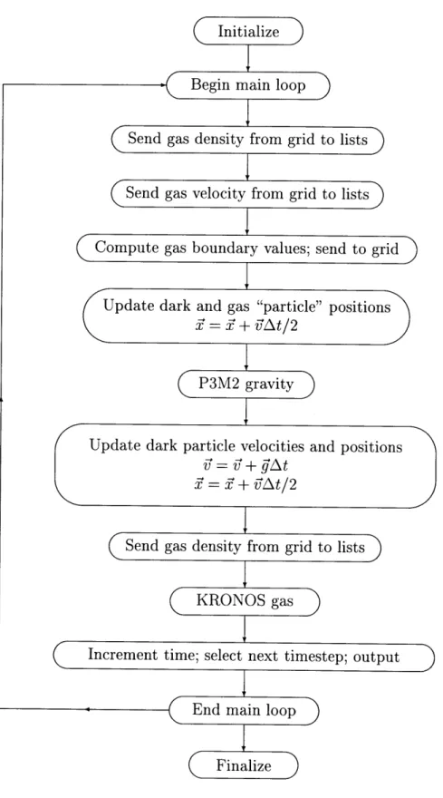
Another advantage of the power ratio statistics is that they are relatively noise free compared to the Mohr et al. (1993) statistics. Figure A-3 shows the emission weighted centroid shift (Eq. 4.7) plotted versus expansion factor. Because a small change in the X-ray image can cause the centers of all the annuli to shift, the centroid shift jumps around from timestep to timestep in the simulation. Compare this to Figure A-9, which shows the power ratios varying smoothly with time. Also note that the difference between the largest centroid shifts and the mean value is a factor of only a few. Comparing Figure A-3 to Figure A-9 shows that the primary merger events show up as peaks in both figures, but that the maximum power ratios are more than 10 times the mean values, making them easier to detect unambiguously. For these reasons we concentrate on the power ratios in our analysis.

4.2

_{Cluster evolution in power ratio space}

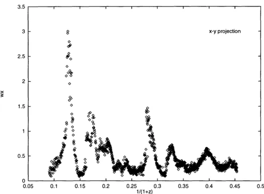
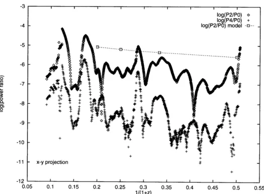
Figures A-4, A-5 and A-6 show the path of the cluster in the space of the P2/PO and

P4/Po power ratios from z = 10 to z = 1 for the x - y, y - z, and z - x projections, respectively. In these plots and the following discussion we take the decimal log of the above defined power ratios and refer to these as power ratios, with the logarithm implied. The high density of points near the center of each of these figures indicates that the cluster spends most of its life near the center of its "territory" in power ratio space. Figure A-7 combines the three projections and shows clearly that this cluster spends most of its life with power ratios -7 < P_{2/Po < -6 and -10 < P4/Po < -8.}

approximately from (P2/Po, P4/Po) = (-8.5, -11.5) to (P2/Po, P4/Po) = (-4, -5).

Between these extremes the allowed region of the plane is a thick filament.

This region of the P2/Po - P4/Po plane was identified by Buote & Tsai (1996),

who interpreted it as an "evolutionary track." They were able to confirm this inter-pretation using 6 simulated clusters, with simulated X-ray images available at only a few redshifts. These plots, showing a nearly continuous path in this power ratio plane, offer spectacular confirmation of their observation.

Closer inspection of these figures reveals that the trajectory of the cluster in this power ratio plane consists of periods in the central part of the allowed region interrupted by excursions out from the center, usually up to the high power region, then down to the low power region, and then gradually back to the center. The excursions to the high power region of the plane generally are direct, progressing up in P₂/Po and in P4/Po simultaneously. Excursions to lower power sometimes occur

in only one coordinate direction, but usually in both.

Physically, what is occurring to the cluster to cause these excursions? In agreement with the interpretation of Buote & Tsai (1996), we find that excursions to high power occur during a merger event. As a subclump of X-ray gas first begins to cross within the 1 Mpc aperture radius for which these power ratios were computed, both the

P2/Po and P4/Po ratios begin to increase. In each case, the P4/Po ratio peaks just

before the P2/Po ratio, and the peak in P2/Po is wider (in time) than the peak in

P4/Po. This can be seen in Figure A-8, in which P₂/Po and P₄/Po are plotted against

expansion factor a = 1/(1 + z) _{for a representative high power excursion. In the plots}

of P₄/Po versus P2/Po this fact is revealed in the clockwise direction in which the

cluster trajectory moves up, around and down in its high power excursions in power ratio space.

For most of the high power excursions the return path in P2/PO - P4/Po space is

a concave path whose shape can be understood in terms of a simple model. Consider the case of a point source with luminosity El1 falling on to a much brighter pointer

source with luminosity E0o. Most of this cluster's mergers consist of single small clumps falling into the main cluster, so consideration of each as a point source can

reveal the qualitative behavior. For this argument we ignore the slight shift in the center of the aperture caused by minimizing P1. When the small source crosses into

the aperture (radius R) surrounding the main source, the powers are given by

P

=

-

,

(4.16)

P4 = 32 o P22. (4.17)

Po is the same for each, so in the P2/Po - P4/Po plane this trajectory is a parabola.

Actual trajectories are more complicated, but qualitatively similar.

Excursions to low power regions of the P2/Po - P4/Po plane take a variety of

paths. Many of these consists of a general decrease, then increase, in both P2/Po

and P4/Po simultaneously. However, there are also excursions which occur parallel to

one power ratio axis or the other. In other words, P2/Po decreases, then increases,

while P4/Po remains almost constant. Or P4/Po cycles down and up while P2/Po

stays fixed. Excursions at fixed P2/Po to low P4/Po correspond to the higher order

components of the X-ray structure of the gas relaxing away, while the m = 2 mode is being preserved by the linear nature of a dominant filament which stretches across the aperture. The P4/Po ratio measures "boxiness," while the P2/Po ratio measures the

linearity of the cluster substructure. Excursions to low P2/Po at fixed P4/Po occur

when the linear nature of the substructure becomes less pronounced relative to the "boxiness."

These types of behavior are indicated by Figures A-9, A-10 and A-11, which show the power ratios plotted versus expansion factor. For an example, study Figures A-9 and A-10, which depict the trajectories in the power ratio plane for the x - y and

y - z projections. At an expansion factor just greater than 0.2, P₂/Po reaches a local

minimum while P4/Po is at a local maximum. This corresponds to the horizontal

low power excursion in Figures A-4 and A-5. This feature is most prominent in the

x - y projection, but the actual sequence of mergers which produce this part of the

trajectory is most clearly seen in the y - z projection of the X-ray surface brightness.

key times in this merger sequence.

Panel A shows the cluster as an X-ray bright clump falls in from above. Both

P2/Po and P4/Po are large. Panel B depicts the situation 15 simulation timesteps

later. The isophote contours in each panel are separated by one decade each, with the highest contour at 10% of the maximum X-ray surface brightness. Because the central luminosity of the cluster has increased, the subclump falling in from above now appears as an elongation of the isophotes. Another, albeit smaller, subclump is falling in from below the cluster center. These two subclumps are not falling exactly radially onto the cluster center. Instead, they will collide just left of the cluster center, as shown in panels C and D. At panel C, P2/Po reaches a minimum, then

abruptly begins increasing. By panel D linear structure is obvious again, although now it is aligned perpendicular to the filament along which the two subclumps entered the cluster. P4/Po has remained relatively constant, at a maximum, as the "boxy"

structure remains, here as a combination of the left-right orientation of the main cluster and the up-down orientation of the main filament. In panel E the left-right alignment cluster is still apparent, and is reflected in the large value of P2/Po. Panel

F shows the left-right structure relaxing away, while a new subclump approaches the cluster from below. P2/Po is still decreasing, but the combination of the remaining

left-right structure in the highest isophotes and the up-down structure imposed by the bottom subclump results in an increasing P₄/Po. By panel G, the dominant structure

is again the up-down alignment resulting from the merger of the bottom subclump. The whole history of cluster mergers of this sort is contained in figures A-13, A-14 and A-15, which show the time evolution of the P₂/Po and P₄/Po power ratios.

Ap-parent in these figures is the "bouncing ball" nature of the trajectories, with more or less rounded peaks separated by "bounces" in which the declining trajectory abruptly reverses itself and begins to rise again to a new peak. This behavior is the norm early in the cluster's history, becoming less frequent as it evolves. The reason for these "bounces" is that mergers are occurring frequently at these early times. After the power ratios peak and begin to decline, but before they can relax to an equilibrium value, a new merger begins as another clump of hot gas falls into the power ratio

aper-ture. The frequency of these high power events decreases with time, as the ever more massive cluster will only show high power ratios when mergers with more massive subclumps occur.

Also evident in figures A-13, A-14 and A-15 is the fact that while the power ratios vary greatly on the timescale of individual merger events, they do not vary greatly on much longer timescales. This can also be seen in figure A-16, in which the amount of time spent at points in power ratio space is shown as a contour plot. The contours are made by overlaying the trajectories in power ratio space for the three projections of the P2/Po - P4/Po, which are shown individually in figures A-4, A-5

and A-6. The points along the trajectories are binned in the P2/Po -P4/Po plane then

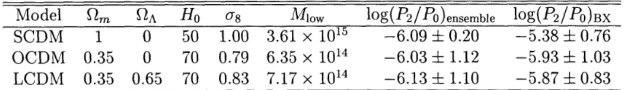
smoothed with a Gaussian. Superimposed on these contours are points corresponding to the power ratios measured by Buote & Tsai for their sample of clusters observed by ROSAT. Of course, the ROSAT clusters are at lower redshift than the simulated cluster. But even over the huge redshift range from z = 10 to z = 1, the cluster occupies the same region of power ratio space as the ROSAT clusters. In addition, the single simulated cluster corresponds to a single perturbation scale, while the data are drawn from clusters with a range of perturbation scales. Still, the shape of the distributions for the simulation and the real data are very similar.

4.3

Substructure survival time

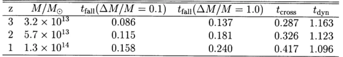
Richstone et al. (1992) and others have argued that the fraction of observed clusters possessing substructure reflects the cosmic mean matter density. In a low density universe, matter approaches free expansion at late times. Consequently, observed structures must have formed early, when the mean density was closer to critical. Clusters formed at early times would have had time to relax and would appear today with little substructure. In order to quantify this effect one requires knowledge of the cluster formation or merger rate as well as the relaxation time scale of the substructure which results from these mergers.

per-turbation in a Friedman-Robertson-Walker universe and assuming a Gaussian dis-tribution for the density on cluster scales, Richstone et al. compute the fraction of clusters which collapse within a certain time interval of the present epoch. If this time interval is chosen to be the amount of time for which evidence of recent merger activity survives, then this fraction of clusters "recently formed" will be the same as the fraction of clusters which show evidence of current or recent mergers. In brief, their argument is as follows.

A homogeneous spherical overdensity above the critical density will collapse at a time which is a monotonic function of the overdensity. A distribution of overdensities then leads directly to a distribution of collapse times as a function of the initial overdensity. The chosen initial density distribution is Gaussian, and its variance is chosen so that the derived fraction of the mass on the scale of 1015_{M® which has} already collapsed is equal to the mass fraction of the universe in Abell clusters with masses of about 1015M0 . Finally, they derive an expression for the fraction of existing clusters which have collapsed within the last time interval 6t.

Applying this expression requires determining the fraction of clusters which show recent merger activity and choosing a value for 6t, which should be the amount of time for which merger activity remains visible in clusters. Interpreting cluster substructure as evidence of recent merger activity, Richstone et al. argue, based mostly on optical studies, that 25% of rich clusters show substructure at present. These authors have concentrated on predicting cluster formation and merger rates and have made simple assumptions about the relaxation time scale of substructure based on the cluster dynamical time or crossing time. They assume that low contrast substructure is erased in about 0.1/Ho. Their results favor Q > 0.5.

Lacey & Cole (1993) perform a similar calculation. They equate the fraction of rich clusters with significant substructure to the fraction of clusters which "formed" within some specified time interval of the present. They define the cluster formation time as that time at which the halo mass first increased to 50% of its present value. They find that matching observations with a CDM spectrum requires Q > 0.6 if they assume that substructure is erased on a timescale of 20% of the present age of the

Universe.

Kauffmann & White (1993) apply the formalism of Press & Schechter (1974) to study the merger history of dark matter halos. They argue that uncertainty in substructure survival time precludes using their results to predict Q from cluster substructure.

Richstone et al. (1992) and Lacey & Cole (1993) both characterized observations of substructure with a single number: the fraction of clusters displaying significant substructure. As discussed in the introduction to this chapter, different observers us-ing different selection criteria have arrived at different values for this fraction, rangus-ing from 20% to 40%. This much variation seems inevitable when there is no consensual definition of substructure. We avoid this dilemma by relying on a set of quantitative statistics, the power ratios, to place each cluster on the continuum of cluster mor-phologies. Then, rather than relying on subjective determinations of the significance of substructure, we simply assign each cluster a set of power ratios. When the sim-plicity of a single number is desired or required, we can, for example, consider all clusters with P2/Po above some threshhold value.

Richstone et al. (1992) and Lacey & Cole (1993) also rely on simple estimates of the time interval during which recent merger activity remains visible as substructure. But these estimates are not rigorous, nor are they well motivated by the details of the substructure measurements.

In this section we study the survival time of the substructure, measured as the duration of high power excursions, in our simulated cluster. In chapter 5 we relate these observations to a simple model for the merging events which produce high power ratios.

Figures A-13, A-14 and A-15 show the time evolution of the P2/Po and P4/Po

power ratios. If substructure survival time is governed by the physics of gas shock-ing, coolshock-ing, and relaxing into hydrostatic equilibrium, then it should be relatively insensitive to cosmology. If, on the other hand, substructure survival time depends on the merger rates of clusters, then the survival time should depend on the cosmol-ogy. As evidenced by these figures, a peak in P2/Po is usually coincident with a peak

in P4/Po and corresponds to the infall of a clump of hot gas onto the main cluster.

The survival time of substructure measured this way is just the width of the peak. Clearly, peak width is relatively constant over the entire range of redshift covered. Meanwhile, the cluster mass evolves significantly, increasing by more than a factor of six between z = 4 and z = 1. Thus, the substructure survival time, as measured by the power ratios, is insensitive to the cluster mass.

Specifically, we define substructure survival time, as related to power ratios, by the full width at half maximum for single peaks in the function P2/Po(t), plotted

in figures A-13, A-14 and A-15. As the vertical scale is logarithmic, a factor of one half corresponds in the figures to a decrement of logo10 2 = 0.3 from the peak. Low peaks which do not fall to one half of their peak value before rising again are not considered single peaks. By this definition, substructure survival time ranges from 0.13 to 0.30 billion years, or about 0.01 to 0.02 Ho1_{. Clearly this is much less than}

the estimate (0.1 Ho1_{) of Richstone et al. (1992), who state that their estimate of Q}

varies approximately linearly with the substructure relaxation rate. Nakamura et al. (1995) provide the following fit to equation 17 of Richstone et al.

Qm > -0.2 _(4.18)

HoRt

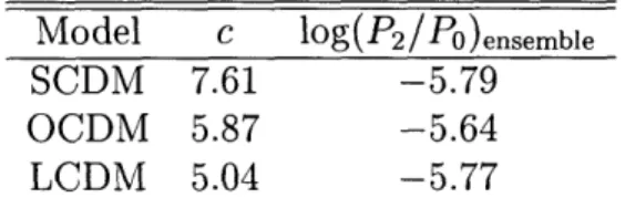
with 6F representing the fraction of clusters which have formed within the last 6t. The implication seems to be that this rate of relaxation indicates a value of Q greater than about 2.5. However, their estimate of Q results from combining an estimate of substructure survival time with measurements of the frequency of occurrence of substructure classified in a certain way, such as the Jones & Forman (1992) morpho-logical classes. A more fair comparison requires using the power ratios to quantify both the frequency of the substructure and its survival time. Evrard et al. (1993) and Buote & Xu (1996) have tried determining substructure frequency in different cosmological models by simulating many clusters in each model. In chapter 5 we develop an analytic model for substructure frequency and survival time that can be used to rapidly test most cosmological models.

Ideally, a large number of hydrodynamically simulated clusters could be used to quantify exactly the expected distribution in power ratio space for a given cosmolog-ical model and as a function of time. Currently that goal is beyond the capabilities of current simulations. However, by using simpler simulations and models for the physics not explicitly simulated, greater numbers of clusters can be generated. Tsai & Buote (1996) used 6 hydrodynamically simulated clusters from an Q = 1 CDM model universe, and found too many high power clusters compared to ROSAT data, indicating Q < 1. In order to get better statistics, Buote & Xu (1996) drew clus-ters from gasless N-body simulations of different cosmologies. To generate simulated X-ray images they assumed Pgas oc PDM and constant temperature. They found that low Q CDM models produce power ratios in good agreement with observations, while

Q = 1 "standard" CDM does not.

While we cannot directly check these results, we can test some of the assumptions that underlie them. Figure A-17 shows the cluster trajectory in power ratio space computed once from the X-ray surface brightness and once again from the square of the gas density. This is equivalent to assuming isothermality. Clearly, the trajectories are very similar, with the isothermal assumption leading to overestimates of the power ratios except at the highest power. This overestimate is due to the fact that the cluster gas temperature is not isothermal; rather, it declines with radius. Figure A-18 shows the spherically averaged gas temperature as a function of radius from the cluster density peak. A similar overestimate is seen for the P3/Po power ratio. By neglecting

this effect, Buote & Xu (1996) would have overestimated the amount of substructure for a given mean density present in their simulations, and hence would have been led to underestimate Q. They argue, however, that the measured X-ray surface brightness is actually the emissivity convolved with the ROSAT detector response function, which varies little over the range of cluster gas temperatures. So the degree to which the isothermal assumption leads to an understimate of Q remains uncertain.

A more significant difference appears when comparing power ratios computed from the X-ray surface brightness and from the square of the dark matter density. Figure A-19 shows the P2/Po power ratios plotted versus expansion factor and computed

from the X-rays, the square of the gas density, and the square of the dark matter density. On average, approximating the X-ray surface brightness as the square of the dark matter density produces significant overestimate of the power ratios. Combining all 3 orthogonal projections of the cluster, we find the mean and root mean square overestimates (in the decimal log of the power ratio) to be 9.3% and 10.5%, respec-tively. Doing the same for the P3/Po power ratios yields mean and root mean square

overestimates of 9.3% and 9.9%. P4/Po overestimates are 10.8% and 11.0%.

Naively correcting for this overestimate in the results of Buote & Xu (1996) means decreasing their value for the mean power ratios for their simulations by 10%. This correction brings their values for the mean power ratios P2/Po and P3/Po for the

standard CDM model into good agreement with the values computed by Buote & Tsai (1996) for their sample of ROSAT clusters. At the same time, this correction destroys the agreement seen by Buote & Xu between the data and their simulations of an Q = 0.35 open CDM model. This reversal of the result of Buote & Xu agrees with the conclusions of Mohr et al. (1995), that the substructure in X-ray clusters is more consistent with a high density than a low density cosmology.

However, this naive correction ignores a point made first by Buote & Tsai (1995), that spatial temperature variations, which are present in the simulated data, are not detected by ROSAT even when present in real clusters. These temperature fluctu-ations arise due to adiabatic heating in collapsing gas subclumps, and due to shock heating which results when a subclump collides with the main cluster or any of the shock fronts present in the cluster. However, the spectral response of the ROSAT PSPC (Position Sensitive Proportional Counter) is nearly independent of the gas temperature (Buote & Tsai 1995, Pfeffermann et al. 1987).

Recalculating the power ratios for our simulation based on the square of the gas density, as opposed to the X-ray emissivity p2_T1_/2_{, results in power ratios closer to}

those calculated from the square of the dark matter density. The result is still an overestimate; i.e., power ratios computed from the square of the dark matter density are higher than those for the square of the gas density. For P2/Po, the mean and root