Control of a nonlinear underactuated system with adaptation, numerical stability verification, and the use of the LQR Trees algorithm

Control of a Nonlinear Underactuated System with Adaptation, Numerical Stability Verification, and the use of the LQR Trees Algorithm

by

Ian Charles Rust

Submitted to the Department of Mechanical Engineering in Partial Fulfillment of the Requirements for the

Degree of Bachelor of Science

at the

Massachusetts Institute of Technology June2010

ARCHVES

JUN 3

0 2010

LIBRARIES

© 2010 Massachusetts Institute of Technology

All rights reserved

The author hereby grants to MIT permission to reproduce and to distribute publicly paper and electronic copies of this thesis document in whole or in part in any medium now

known or hereafter created.

Signature of Author...

Certified by ...

Professor of Mechanical Engineering,

Accepted by ...

Department of Mechanical Engineering Ma 10, 2010

Jean-Jacques E. Slotine Professor of Brain and Cognitive Sciences Thesis Supervisor

... ... ... -a--... ... ...

II~hIIJohn

H.

Lienhard V

Control of a Nonlinear Underactuated System with Adaptation, Numerical

Stability Verification, and the use of the LQR Trees Algorithm

by

Ian Rust

Submitted to the Department of Mechanical Engineering on May 10, 2010 in Partial Fulfillment of the Requirements for the Degree of Bachelors of Science in

Mechanical Engineering

ABSTRACT

Underactuated robotics, though surrounded by an established body of work, has certain limitations when nonlinear adaptive control principles are applied. This thesis applies a nonlinear adaptative controller that avoids many of these limitations using alterations inspired by the control of a similar underactuated system, the cart-pole. Due to the complexity of the system, a sums-of-squares MATLAB toolbox is used to generate a suitable Lyapunov Candidate used for proofs of stability, with claims of local stability made using Barbalat's Lemma. This provides us with a local domain of attraction for the altered classical nonlinear adaptive controller. In addition, the algorithm known as LQR Trees is applied to the system in order to create a controller with a larger region of attraction and lower torque requirements, though without an adaptive component. Both control systems are implemented in simulations using MATLAB.

Thesis Supervisor: Jean-Jacques E. Slotine

Table of Contents

ABSTRA CT ... . -.. ---... 2

LIST O F FIG URES... 4

INTR O DU CTIO N ...---.. 6

PROPOSAL OF THE CYLINDER-BEAM SYSTEM... 7

BACKGROUND ON ADAPTIVE CONTROL ... 11

BARBALAT'S LEMMA... ...----..--- 14

EXPANSION TO THE UNDERACTUATED CASE... 15

IMPLEMENTATION OF ADAPTIVE CONTROL ... 17

EXPANDING THE ADAPTIVE CONTROLLER FOR UNDERACTUATION ... ... ... 18

TH E O BSERVER...- 23

STABILITY O F TH E LIN EARIZED SY STEM ... 25

REG IO N O F ATTRA CTIO N ... 28

LQ R TREES ... 36

GROW ING THE TREE...---... 39

THE TIME-V ARYING LQR CONTROLLER ... ... ... ... 42

REGION OF ATTRACTION OF A BRANCH... 44

APPLICATION OF THE CONTROLLER... 46

CO N CLU SIO N ... 49

APPENDICES ... 51

REFEREN CES... 54

List of Figures

FIGURE 1 - A BASIC REPRESENTATION OF THE CONTROLLER DESIGNED FOR IN THE LQR TREES ALGORITHM. 7

FIGURE 2 - A BASIC SCHEMATIC OF THE ROBOTIC SYSTEM PROPOSED FOR THE PURPOSE OF STUDYING

UNDERACTUATION, NON-LINEAR CONTROL, ADAPTIVE CONTROL, AND THE LQR TREES ALGORITHM.. 8

FIGURE 3 - CHOICE OF GENERALIZED COORDINATES FOR DERIVATION OF THE DYNAMICS OF THE SYSTEM .... 9

FIGURE 4 - C ART-POLE SYSTEM ... 19

FIGURE 5 -U NSTABLE FIXED POINT ... 22

FIGURE 6 - STABLE FIXED POINT ... 22

FIGURE 7 - RANGE OF C IN WHICH ALL EIGENVALUES OF THE A MATRIX ARE NEGATIVE... 27

FIGURE 8 - STABLE CASE OF THE CONTROLLER. ... 29

FIGURE 9 - UNSTABLE CASE OF THE CONTROLLER... ... 30

FIGURE 10 - LYAPUNOV CANDIDATE AND ITS TIME DERIVATIVES PLOTTED FOR THE STABLE SIMULATION... 32

FIGURE 11 - LYAPUNOV CANDIDATE AND ITS TIME DERIVATIVES PLOTTED FOR THE UNSTABLE SIMULATIO 33 FIGURE 12 - REGION OF ATTRACTION BASED ON ANALYSIS OF A LYAPUNOV CANDIDATE FUNCTION AT VARYING INITIAL CONDITIONS FOR a AND

a

FIGURE 13 - REGION OF ATTRACTION BASED ON ANALYSIS OF A LYAPUNOV CANDIDATE FUNCTION AT VARYING INITIAL CONDITIONS FOR

9

9

FIGURE 14 - REGION OF ATTRACTION BASED ON ANALYSIS OF A LYAPUNOV CANDIDATE FUNCTION AT VARYING INITIAL CONDITIONS FOR a AND d.. ... 35 FIGURE 15 - REGION OF ATTRACTION OF THE TIME INVARIANT LQR CONTROLLER SEEN IN THE a,

a

PL A N E . ... 3 8 FIGURE 16 - REGION OF ATTRACTION OF THE TIME INVARIANT LQR CONTROLLER SEEN IN THE 9, 9 PLANE..

... 3 9 FIGURE 17 - EXAMPLE OF TRAJECTORY OPTIMIZATION FOR RANDOM INITIAL CONDITIONS SEEN IN THE a, d

PL A N E ... 4 1 FIGURE 18 - EXAMPLE OF TRAJECTORY OPTIMIZATION FOR RANDOM INITIAL CONDITIONS SEEN IN THE 9, 9

FIGURE 19 - REGION OF ATTRACTION OF CONTROLLER AFTER ADDING 2 BRANCHES, PROJECTED ONTO THE , d PL A N E . ... 4 5

FIGURE 20 -REGION OF ATTRACTION OF CONTROLLER AFTER ADDING 2 BRANCHES, PROJECTED ONTO 9, 9 PL A N E . ...---.-.-... 4 5 FIGURE 21 - SIMULATED TRAJECTORY STARTING FROM A RANDOM POINT WITHIN THE BOUNDS OF THE TREE,

SEEN IN TH E a , a PLA NE. ... 47

FIGURE 22 -SIMULATED TRAJECTORY STARTING FROM A RANDOM POINT WITHIN THE BOUNDS OF THE TREE, SEEN IN TH E 9 , 9 PLAN E ... 48 FIGURE 23 - CONTROL INPUT FOR THE TRAJECTORY SIMULATION SEEN IN FIGURES 21 AND 22. ... 48

Introduction

The control of underactuated systems, though often complex, has an established body of work. As a first step, linearizations can be made, which allow for linear control principles to be applied. These sorts of strategies can be effective, though they are limited due to the fact that all linearizations are based on approximations. When applied to the real system, these approximations only serve to limit the effectiveness of a controller and region of stability of the controller.

Lyapunov analysis is particularly useful as it allows one to avoid this need for linearization. The real dynamics can be used, and as such claims on the stability of the real, nonlinear dynamics can be made. For example, a Lyapunov candidate, a function of the state of a system, is defined as:

V(x) ₍₁₎

If this function is positive definite, and its time derivative is negative definite, then the

system is locally stable at the origin. If the function has the following property:

V(x) -> oo as x -> oo (2)

Then the system is globally stable. There is no need for linearization, and a rather strong claim of stability is made [5].

In addition, adaptation follows quite simply as an extension of this stability analysis (with related analysis using Barbalat's Lemma and the Invariant Set Theorem). This is convenient, since, like linearizations, most models are simply approximations. As is discussed in this thesis, canonical Lyapunov-based proofs of stability for adaptive systems have a distinct reliance on full actuation. In addition, viable Lyapunov candidates are often extremely difficult to determine to for complex systems.

This thesis studies a unique underactuated system as a tool in exploring what claims can be made on the stability of an underactuated system. The system has certain properties that make adaptation applicable, and as such is a suitable platform for study.

Numerical tools are used in order to generate a Lyapunov candidate for the system, and this candidate allows us to detail the regions of local stability in state space.

However, the ultimate goal is to have a globally stable controller. Since we know that claims of local stability can be made, this thesis uses a series of local, linear LQR controllers which covers a larger area of the state space than a single local controller. These controllers are connected in a "tree" in which trajectories are moved from one region of stability to the next until they reach some desired point in state space. In this way all trajectories are simply be "funneled" to the desired point.

Figure 1 - A basic representation of the controller designed for in the LQR trees algorithm. In the algorithm, the "funnels" are not all stable about a point, but also are stable about trajectories. Notice how a trajectory might cascade from one "funnel" to the next. [8]

The controller applied is simply a function of where in this tree the trajectory is (i.e. the gain matrix is changed depending on where in state space the trajectory is). This is an application of the LQR Trees Algorithm [8]. For simplicity, this task is done without adaptation. Future work may seek to synthesize these two approaches; however that is beyond the scope of this thesis.

Proposal of the Cylinder-Beam System

The underactuated system studied in this thesis is a somewhat complex "toy" robotic system with a biological inspiration. Consider the real situation of a pen balancing

upon a human finger. The finger has a number of inputs which can control the position of the pen on the top of the finger, most of which involve the finger moving in

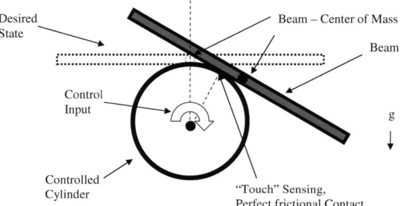
three-dimensional space with six degrees of freedom (translation in three directions and rotation about three axes). The robotic system attempts to emulate this biological balancing system, with certain simplifications. The first is that the system must be constrained to two dimensions. In addition, the control input is reduced to only one control torque, resulting in one rotation. This system thesis called the cylinder-beam system for the remainder of this thesis. It is named as such because it replaces the "finger" with a cylinder forced to rotate about its center and it replaces the "pen" with a beam, forced to only move in two dimensions. This beam is also constrained by a "perfect" frictional contact in which there is no slipping between the beam and ball and they always remain in contact with one another.

Desired Beam - Center of Mass

State

Control

Input _g

Controlled

Cylinder "Touch" Sensing,

Perfect frictional Contact

Figure 2 - A basic schematic of the robotic system proposed for the purpose of studying underactuation, non-linear control, adaptive control, and the LQR Trees Algorithm.

This system has several unique properties. The first of these is the fact that there exists "touch" sensing. What this means is that the position and velocity of a contact point between two rigid bodies in the system is measured. In this system the contact point between the beam and cylinder is tracked in this way. The second is the rather

unconventional rolling contact between the two bodies, the cylinder and the beam. The beam is able to roll about the cylinder, meaning it is rolling about the contact point.

However, the contact point moves with the beam, making the dynamics somewhat complicated.

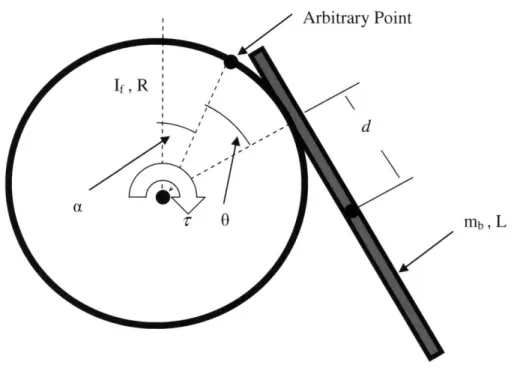
In order to derive the dynamics of the system, generalized coordinates must be decided upon. For this system, two angles, 0 and a, are able to adequately describe the state of the system (along with the time derivates of these angles). This gives us four states for this clearly fourth-order system

Arbitrary Point

I0m, R

d

0

6Mb , L

Figure 3 -Choice of generalized coordinates for derivation of the dynamics of the system through Lagrangian mechanics. The coordinate a is the angle of an arbitrary point on the cylinder to vertical. The coordinate 0 is the angle from the contact point to the arbitrary point a is in reference to. For complete explanations of the system parameters shown above, refer to Appendix 1.

As seen in Figure 3, a is defined as the angle between an arbitrary point on the cylinder

to vertical and 0 is defined as the angle between this arbitrary point and the contact point. Other important parameters of the system include the distance of the center of mass to the contact point, denoted as d , which is a function of 9 and a constant length do .

Once this has been done, the equations of motion can be solved for using the methods of Lagrangian Dynamics. For numerical values of the constant parameters in these

equations, refer to Appendix 2.

12 d+ +)+mRd($-&)($+&)+mb gd cos(a+0) = 0 12 (d+N +Id+2mRd($+&)$+ m g (d cos(a+0)- R sin(a+0))=

Il=If+mbR2

L2=MPd2

I2 =mb -+d2

12

This can be rearranged into the more classical form:

H (q)4 + C(q, 4)4 + G(q)= q= I _I

H(q)=2

=

1212

11

1

This verifies the conservation of energy condition [5].

4T(5

-2C) 4=0

The desired state of the system is to have the beam directly on top of the cylinder. What this implies is that the center of mass must be directly vertical and in contact with

the cylinder. Incidentally, these conditions correspond to 9+ a =0 and d = 0, respectively. Therefore, the following desired trajectories for the state variables are found: d (14) R d _ (15) ad-R 0d =0 (16) ad = 0 (17)

One problem with these desired trajectories is that the overall objective of the adaptive control used in the control system presented in this thesis is to stabilize the beam using no prior knowledge about the beam. The constant do is not something that can be directly sensed, and falls under the domain of information about the beam, more

specifically the way in which it first comes into contact with the beam. Therefore, as thesis explored in much more depth later in this study, an observer is needed to determine an estimate of the constant do .

The control system applied to this robotic system uses several principles of nonlinear adaptive control. The following sections will detail how these principles are applied to this system, as well as where they must be refined and altered in order to accommodate for various complexities inherent in the system. The most notable of these complexities, of course, is underactuation. In order to fully understand the approach to underactuation, we must look at how adaptive control using a sliding variable controller is implemented and how its stability is verified for a fully actuated system.

Background on Adaptive Control

Adaptive control in fully actuated, nonlinear systems has a well-established body of work [5]. These tools are particularly useful, as stability can almost always be

Barbalat's Lemma). Fully actuated systems are common, as are error in parameters such as mass, damping, etc. Without adaptive control, imperfect models would be used, which lends itself to an imperfect controller. Therefore, this particular strategy of control is important and is fortunate to have clear, established proofs of stability. A typical adaptive controller begins with typical autonomous dynamics, written in the general form:

H(q)ij + C(q, 4)4 + G(q)= r (18)

In order to control this system, a sliding variable must be established. A typical sliding variable is defined as such:

s =

4+24

Where

4

S+24 =0 (20)

This system has clear global exponential stability. Therefore, by controlling the sliding variable, both position and velocity of the system can be controlled. Further definitions using this sliding variable will be particularly useful in establishing the basis for adaptive control in this thesis.

s = q - (21)

4 4d -24 (22)

In these equations, 4,. is a reference of sorts for the sliding variable.

Returning to the adaptive controller, the analysis used to show the stability of the controller is similar to Lyapunov Analysis, and involves a Lyapunov Candidate Function:

V =I (sTHs+5T -) >0 (23) 2

Where F-1 is a negative definite matrix and 5 is the error in the adaptation parameters, defined as = a - a. This defines V as a positive definite function, which allows for

future claims on stability to be made. The variable a is a constant vector describing the mass and other unknown parameters of the system. This constant vector is chosen such that H (q), C(q, 4), G(q) all have the following linear relationship with a:

H (q)4i, +C(q,4)4, +G(q) = Y(q,4,4,,ij,)a (24)

The reason for this becomes more evident once the Lyapunov candidate is differentiated with respect to time:

Y = sT(Z-_Hj, --C, - T-I (25)

After substituting equation (24) into (25), this becomes:

V= sT(r-Ya)+NTF-in (26)

This definition allows us to choose control and adaptation laws that, in the style of Lyapunov analysis, make this negative definite. The choices for control and adaptations laws are as such:

S=Y - Kds (27)

ii =- FYTs (28)

V =-s TKds < 0 (29)

This is a negative definite function. Yet, since it is not a function of all states (a has its own dynamics) it cannot be examined with traditional Lyapunov Analysis. However, Barbalat's Lemma will prove a useful tool in proving the stability of the system [5].

Barbalat's Lemma

Barbalat's Lemma is used to prove the local stability of the classical nonlinear adaptive controller detailed previously. In addition, its basic principles are used to show stability in certain regions in the underactuated system studied in this thesis.

Barbalat's Lemma, in its simplest form, states the following:

If:

-The differentiable function f(t) has a finite limit as t ->

-

f

Then f(t) ->ooas t ->oo

Applied to Lyapunov-like functions, the following corollary is made:

If:

-V(x, t) is lower bounded

-V(x, t) is negative semi-definite

-V(x, t) is uniformly continuous

For the Lyapunov candidate in the previous section already has been shown to satisfy the first and second criteria. For the third criterion, is verifies by examining the closed loop dynamics:

H+(C + Kd)s =Y5 (30)

From this, if s and 5 are bounded (which comes from equation (29)), i is bounded. This means that V is uniformly continuous, since V is defined as:

V = -s TKdi (31)

This shows that V -+ oo, and therefore s ->0 as t -- oo. This in turn guarantees q

converges to the specified desired trajectory [5].

Expansion to the Underactuated Case

In the preceding discussion of adaptive control, certain conclusions are

consequences of the system being fully actuated. The most important concern is with the definition of the control law, repeated below:

r =Ya - Kds (32)

For a system with dim(r )=m, this equality can only be enforced if Z is entirely non-zero entries. However, this criterion directly correlates to the definition of an underactuated system.

The definition is as follows [7]. For a system with following general definition:

ij= f1(q, 4, t)+ f2(q, 4, t)u (33)

(34)

Returning to the adaptive case, an entry of zero directly corresponds to an

f

a rank of m-r, where r is the number of zero entries in the system. Since dim(q)=dim(r ), a zero in r means that the system is underactuated. Therefore, if a system is

underactuated, the inputs needed for in the control law for the conventional adaptive control can no longer be applied to the system (some of the inputs will always be zero). This basic difference invalidates the control strategy stated in detail in previous sections. The remainder of this thesis is spent finding a viable substitute for this control system.

To begin, Partial Feedback Linearization (PFL) is used on the cylinder-beam system in order to minimize the effects of the dynamics of 9 on the dynamics of a [6]. This particular type of partial feedback linearization is called collocated PFL, since a is the variable which is directly affected by the control input. This is done simply by subtracting (4) from (5). This yields the following dynamics for a:

Ild+mbdOR(+ &)2 +mbR 29(#+ d) 2 -- m gR sin(9+a) = r (35)

This use of collocated PFL allows for the dynamics of the system to be reduced to a linear relationship between some dynamical vector Y and a constant vector a.

Ic,+mbdoR($+&)2 +mbR 20 + d)2 -m gR sin(9+a) =Y (a,&, )a (36)

Where Y and a are defined as:

Y(a, &, ,)= d[a, (#+d)2 _0(#+d)2 _{sin(6 +}

_a)

a =[I, mbdOR mbR2 mbgR] (38)

=a

-2&(39)

Of course, non-collocated PFL is another option for simplifying the dynamics of the

system for use in adaptation. This would mean that the effects of the dynamics of a on the dynamics of 0 are be minimized. When this is performed, the following dynamics for

9 are found:

,##+(9+)(mbRd(5-d)-2mRd5)+msg ((1-$3)dcos(9+a)+#,Rsin(9+a))=-$r (40)

1112

(41)

, +I2

This equation again indicates a linear relationship between a dynamic vector and constant vector, though this relationship would be unnecessarily complex to detail in full in this thesis. The collocated PFL found in equation (35) plays an identical role, and is much simpler. Therefore, it is used as the stability characteristics of the controller proposed in this thesis are explored.

Implementation of Adaptive Control

Equation (36), found through collocated PFL, allows for us to design an adaptive controller exceedingly similar to classical controller detailed previously. This begins by choosing a similar Lyapunov candidate function.

V

In this the sliding variable is defined in terms of the error Cc.

s=a+2 ~ (43)

a a-ad (44)

Where ad is the desired trajectory for a. As was the case for the classical controller, the adaptation and control laws take on the following form:

r =Y -KdSa (45)

a = -FYTSa (46)

Y is the vector of state-dependent dynamic terms detailed in full in equation (37). With

these definitions, the derivative of the Lyapunov function can be reduced to a negative definite function.

Y=-Sa

Through Barbalat's Lemma, in an identical proof to that seen in equations (29) through

(31), it is shown that V -+ oo, and thus a tends towards the desired trajectory.

This is a perfectly valid controller, however it only stabilizes a, and makes no claims on the stability of 9. In order to ensure that 9 is also stabilized, additional terms must be added to the control law. The next section details one strategy for doing this, and provides some background on another underactuated system which uses a similar strategy to confront an equally similar problem.

Expanding the Adaptive Controller for Underactuation

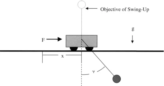
The strategy for control of the non-collocated variable 9 is exceedingly similar to the control of the collocated variable x seen in the cart-pole system shown in Figure 4. The cart pole is a relatively simple system, though it is underactuated and has distinctly nonlinear dynamics. In it, a force is applied to a cart which is constrained to move along a line, parameterized by x. Attached is a mass that is fixed to rotate about some point on the cart (the "pole"). The overall objective of the control system is to swing the pole to the top of the cart, as well as to place the cart at some point in x (usually x=0 )

Objective of Swing-Up

g

F p

x

Figure 4 -Cart-Pole System. A control strategy used for this system is adapted to the cylinder-beam system. In this system, a force can be exerting laterally on the cart.

Energy-shaping control is often used in order to swing the pole above the cart. This is an effective tool for this situation, for if the energy of the system always approaches the energy of the system when the pole is directly above the cart and all velocities are zero, only two situations can exist. The first of these is that the pole will eventually be directly above the cart and all velocities are zero. This occurs when the initial energy is anything but the desired energy. The second is that, if the energy is already the desired energy, the system will stay in its current state. This second situation is unrealistic, but in either situation the pole is in the desired location. As such energy shaping is an excellent choice for swing-up control.

As an aside, energy shaping control, as it is seen in the cart-pole system, may seem like a suitable choice for controlling the cylinder-beam system. However, for reasons that are not the focus of this thesis, the cylinder-beam system is unsuited to energy shaping control since the system is not constrained in the vertical direction like the cart-pole. What this means is that the cart pole is unable to move vertically beyond simply rotation of the pole. The beam in the cylinder-beam system is only fixed by a frictional constraint. This means that the potential energy of the system has no lower boundary. As such, it can assume a trajectory that allows the energy to converge to a

desired point by simply having fallen off the side of the cylinder, with increasing kinetic energy. The kinetic energy gained in speeding up during the fall is compensated by a loss

of gravitational potential energy. As such, a stable trajectory in terms of energy can be

highly unstable in terms of the parameters that the controller would seek to stabilize.

The dynamics of the cart-pole, for the purposes of this thesis, are inconsequential. The most important aspect of the dynamics is the fact that with a suitable choice for a control results in an exceedingly useful property of the energy of the system. Note that this is done using collocated PFL [1].

Z

Z=

K>O (50)

As can be seen in these "dynamics" for the energy, the error of the energy, defined by

some desired energy Ed, tends towards zero as t -> oo. Therefore, the pole is swung-up

to the vertical position.

However, there are no claims in this controller on the stability of the state x. Therefore, some terms must be added in order to shape the behavior of this state. The obvious choice for this is the simplest. A linear, PD (proportional and derivative) for x is placed in the control input. Therefore, the force input (with unit masses, lengths, etc.) becomes:

F = [(-sin ycos y-

f

v = k?cos yE - Kx - K2x (52)

This system has proven stability, despite the fact that the convergence of the energy seen in equations (29) to (31) is no longer valid. This is shown using Floquet Theory, which begins with linearizing the dynamics of the system about a periodic trajectory. The

stability of this is verified by checking the stability of the transverse dynamics along this trajectory [3]. The full details of this particular stability verification are not the topic of this thesis, as the transverse dynamics of the cylinder-beam system are entirely different.

Returning to the cylinder-beam system, this same philosophy is used in order to stabilize 9 in the cylinder-beam system. Just like in the cart-pole example, we add PD terms to the controller seen in equation (45) in order to stabilize 9. However, since

9= - is already a stable fixed point (upon examining the dynamics in equation (4)),

R

all that is required is a derivative term. The existence of this fixed point can be shown by first setting all time derivatives in equation (4) equal to zero. When this is done, the following fixed points are found:

a+=

2' 2 2

_=-do

(54)

R

However, the first of these is an unstable "fixed" point, while the second is a "stable" fixed point. This is shown by linearizing the system about each of these points. In addition, a is fixed in order to purely show the dynamics of 9. For the situation in equation (53), the general solution of 9 indicates instability. For the situation in equation

(54), the general solution of 9 indicates marginal stability. This can be seen by

examining the general solution of these two modes (numerical answers are found using the parameter values in Appendix 2).

8

general,unstable = c0.2009e4_7 5 3t -c0.2009e 4.8753t (55)

,generalstable = (coO.2e4.8999it -c 10.2e -4.8999i')i (56)

For a physical understanding of this, the first fixed point corresponds to the beam perched on left or right edge of the cylinder, with a vertical orientation. This is intuitively unstable (it is much like the vertical point in the cart pole).

a+O=

(2n+1)-2

Figure 5 -Unstable fixed point in which the beam is perched on the edge of the cylinder. This situtation is intutively unstable, as it is similar to the vertival position on the cart pole.

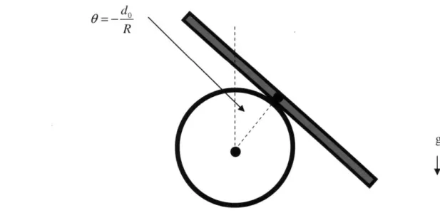
The second of these fixed points consists of the beam having its center of mass at the contact point. This is intuitively stable, as then there would no longer be a torque about the center of mass, and as such 9 would not vary (though a can).

0=-d

R

Of course, intuition would also say that additional PD terms would not be detrimental.

However, further analysis in this thesis on numerically computing region attraction for this controller has shown that the region shrinks considerably with this term, though the causes are unknown.

Since a proportional term is no longer needed, the control and adaptation laws take on the form:

=Y& - Kdsa -cKd (57)

a = -FYTSa (58)

This, like the cart-pole system, has dubious stability properties once the linear control terms are added. Instead of verifying stability using Floquet Theory, this thesis uses local stability verification using Lyapunov-like analysis with Barbalat's Lemma. In addition, the gain scaling factor c must be tuned using checks for stability. For complete details of the other control constants used in simulation (F, Kd , etc.) please refer to Appendix 3.

This system is fairly complex, and as such suitable Lyapunov candidates are exceedingly difficult to find. Fortunately, many numerical tools are available in order to compute Lyapunov functions. The most notable tools are sums-of-squares tools, which are useful because they are able to reduce tests of positive definiteness of a function to a test of positive definiteness of a matrix (something much easier and faster to compute). Future sections of this thesis discuss the implications of the candidate Lyapunov function

generated using this method.

The Observer

The goal of the control system designed in this thesis, in a broad sense, is to stabilize the beam on top of the cylinder with no knowledge of the beam altogether (other than the fact that it can be modeled as a two-dimensional "line" of uniform mass

distribution). The adaptation implemented in this controller is the first step in achieving this goal. The second and final step toward estimating the parameters of the beam is to

design an observer in order to determine the position of the center of mass of the beam, do

-The necessity of the observer for this constant is apparent in the fact that the desired points for both 9 and a are functions of this value. Therefore, if the beam is ever to be stabilized atop the cylinder, this value must be estimated and fed back as a reference for each of these states, 9 and a.

Fortunately, there is a rather simple choice for the observer, and has an equally simple explanation of convergence. The observer is designed to have the following dynamics:

d0 =-d0 -R (59)

In essence, this results in do being a first-order low-pass filtered version of -R9, with a cutoff frequency of 1 rad / s . Upon examining these dynamics, several observations can

d

be made. The first is that when 9= 0 , do =0. This means that if the controller R

detailed previously is able to control 9 to this value, the observer converges to some constant value. Therefore, we replace the previous desired trajectories (seen in equations (14) through (17)) with the following desired trajectories:

0

do(60)

Therefore, do converges to a constant value if the controller succeeds in stabilizing 9 to the desired value detailed above. However, this makes no claim on exactly what constant value to which this observer converges. This constant value can be

determined by examining the dynamics (equation (4)). Once again the assumption is

made that the controller is stable (at least for some region) meaning that as t -> 00, a, 9,

d, d approach the desired trajectories detailed in equations (60) through (63). When this

occurs, the dynamics in equation (4) are reduced to a simple equality:

d0 -do =0 (64)

This shows that do -> do in the case of a stable controller. Therefore, if this observer is implemented, there is a conditional convergence for do . If the controller is stable, then

do -> do . If it is not, no further claims can be made. In summary, if stability for the controller can be verified, then the conclusion can be made that the observer converges to the desired value.

Stability of the Linearized System

The first step in stability verification for the controller designed in this thesis is to linearize the system about the fixed point of the system. This point is detailed as being the point at which a and 0 each are at their ultimate desired points (i.e. the state at which we seek to stabilize all trajectories towards).

-d0 ,desired Ro (65) R d adesired _ (66) R desired (67) adesired =0 (68)

a =constant (69)

do =do (70)

Linearization begins by first taking the Jacobian of the nonlinear system, and evaluating it at this desired point. However, since the controller adds four new state variables from the adaptation law and the observer adds one new state variable due to the dynamics of the observer, the order of the system increases. Before the controller and observer were implemented, the system was fourth order. However after the controller and observer are implemented, the system is ninth order. The linearized dynamics of the system therefore can be reduced to:

f(x)

ax X=Xdesired

x a a, a2 a3 a4

d

(72)

When this is done for the closed loop system, the following A matrix is found:

0 0 1 0 0 0 0 0 0 0 0 0 1 0 0 0 0 0 2_I 1, -mgR+(c-1)Kd Rg mL2 +12I, K cK± I _ Kd +I 0 0 0 0 21+cK I L2 1I, ) I Id 10 RI mgR 2I₁,+mbgR+(1-c)Kd K cK +I Kd 1, 0 0 0 0 21 +cKd A =t I, II I it RII, 73 0 0 0 0 0 0 00 0 0 0 0 0 0 0 0 0 0 0 0 0 0 0 0 0 0 0 0 0 0 0 0 0 0 0 0 -R 0 0 0 0 0 0 0 -1

In order to examine the stability of the system, the eigenvalues must be calculated. For this to be done, the system parameters found in Appendix 2 and the control parameters found in Appendix 3 were substituted in. Using c =1, the following eigenvalues are found:

2=[9.5564+35.2196i 9.5564-35.2196i -15.9595 -1.3118 0 0 0 0 -0.8415] (74)

One complex eigenvalue pair is unstable. However, this can be remedied by changing the value of c. There are also four zero eigenvalues. These correspond to the four adaptation states. This merely means that these states will be constants at this point. In addition, the point at which the linearization is centered for the adaptation states does not affect these eigenvalues.

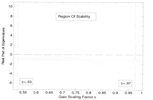
In order to determine the stability as a function of c, the real parts of the

eigenvalues were calculated for the values 0 < c < 1. All values of c that resulted in all negative (or zero) real parts of the eigenvalues were considered acceptable values, as this denotes a stable system. A graphical representation of the results can be found in Figure 7.

0.55 0.6 0.65 0.7 0.75 0.8 0.85 Gain Scaling Factor c

0.9 0.95 1

Figure 7 -_{Range of c in which all eigenvalues of the A matrix are negative (or 0 in the case of the} adaptation dynamics). Note that this criteria is primarily dictated by on eigenvalue in particular, and the dashed lines show the transition from stable eigenvalues to unstable eigenvalues.

Upon examining these results, it was found that the range of acceptable values of c

(those that resulted in a stable linearized system) was:

0.53 < c <0.97 Region Of Stability

- c=.53 _c=.97

For the remainder of the study, c is picked to be 0.9. This results in the following stable eigenvalues (real parts are negative):

2=[-3.1840 +15.1475i -3.1840 -15.1475i -90.2546 -0.8469 0 0 0 0 -1.2811] (76)

Therefore, the linearized system about the desired fixed point is stable, with the exception of the adaptation variables. They are marginally so, but are fixed as constants in this linear domain as seen in the zero entries in the eigenvalues seen above. The following analysis is concerned with discovering when the controller is able to successfully move the system state to the fixed point of this linearization.

Region of Attraction

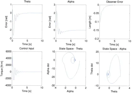
With the case of fully actuated nonlinear control, a concise proof can be made on the stability of the global stability of the controller. However, underactuation increases the complexity of this proof immensely, and therefore this thesis uses numerical tools in order to explain the stability of the controller. In addition, this controller is not globally stable. There are certain sets of initial conditions that are stabilized, and certain initial conditions that are not stabilized. To show this, the control system was applied to the system in simulation for two sets of initial condition, one unstable, and one stable. For this, the system and controller parameter values found in Appendix 2 and Appendix 3 were used (note especially that Kd was set to be lx 103_{). The first, the stable case, had}

the following initial conditions:

x=[ 0 0 0 0 0 0 0 0 (77)

'4

do = 0.1m (78)

Note that the initial length, do , while like an initial condition, also characterizes the dynamics. This means that different values of do will yield a different dynamical system,

which can be seen in the existence of this constant in the dynamics. The results of the simulation showed stability:

Theta Alpha Observer Error

0 2 W 0 5 10 Time [s] Control Input 6000 4000 2000 1 0 1 -2000 -4000 0 5 10 Time [s] -0.051 -0.15 1 5 10 Time [s] State Space - Theta

-2 0 2

Alpha

Time [s] State Space - Alpha

-10'

-2 0 2 4

Theta

Figure 8 -Stable case of the controller. Position errors are in reference the desired trajectory (a function of the observed parameter do ).

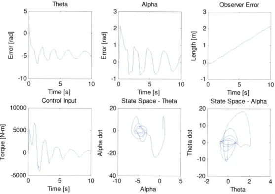
In comparison, the controller is unstable with slightly different initial conditions:

x= 0 2 0 0 0 0 0 0

14

(79)

(80)

do =0.1m

When the exact same controller is acting, and these slightly different initial conditions are applied, the following behavior is seen:

Theta -10 1 0 5 10 Time [s] Control Input 10000 5000 0 -5000 0 5 10 Time [s] Alpha 0 5 10 Time [s]

State Space - Theta

-5 0 5 Alpha Obsener Error 3 2 0 -1 0 5 10 Time [s]

State Space - Alpha

20 10 -10 -20 -2 0 2 4 Theta

Figure 9 -Unstable case of the controller. Position errors are in reference the desired trajectory (a function of the observed parameter do ). Note the slight variation of initial conditions as compared to the stable case.

It can be seen from these two cases that the controller is only locally stable, meaning that it only stabilizes the system for a specific set of desired initial condition. As stated previously, computational tools are well suited for this particularly complex case. Sums-of-squares tools are applicable to this problem, as they are able to reduce tests of negative and positive definiteness for functions to tests of positive definiteness of a matrix. For example, take the simple polynomial:

1+2x2 ₍₈₁₎

By examination, this is obviously a positive definite polynomial. That is not as easily

seen computationally. Yet, one observation that can be made is that this polynomial is exactly equivalent to the following:

[ ]1 0][ 1 X Ax (82)

10 2 x

This product is always positive definite, if the matrix A is positive definite. This comes directly from the definition of a positive definite matrix.

xTAx >0 for any x (83)

In cases of much larger polynomials, this insight allows for rapid tests of positive definiteness in a computational environment. There has been a toolbox written for

MATLAB which uses this for various goals. The toolbox is SOSTOOLS, and it is used in this thesis to determine the region of attraction for the controller [4]. This is done by simply solving for a Lyapunov candidate function which would satisfy Barbalat's Lemma for a certain region. This is in turn done by ensuring that the candidate function is

negative definite for this region, which is the same as a test for positive definiteness, except the A matrix used is -A.

One unfortunate aspect of this sums-of-squares method is that it requires tests of positive definiteness to be done with polynomials. Therefore, the sinusoidal terms in the dynamics cannot be used. Instead, they must be replaced by Taylor expansions about the stable point, a+0=0

N (-1)" (84) sin(a+ ) (a+ 9)2n+1 n= (2n + 1)! N (-1)" (85) cos(a+6)=Z (a+69)2_. n=1 (2n)!

N is chosen to be as large as possible such that computation is not unnecessarily slow (N = 2 for the following analysis). This allows for a search to be made for a positive definite function with a time derivative that is negative definite, using the dynamics of the closed loop system. This was first done by doing searching for a function with these properties globally for the whole of state space (for the case of do =0 ). Obviously, from

our results seen in Figure 8 and Figure 9, this is impossible, and the algorithm halts citing potential "infeasibility" in the problem.

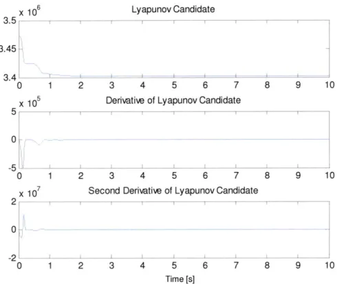
However, it does leave us with the current "best guess" for a function of this nature (simply the last function solved for during the iterations of SOSTOOLS), which will prove useful. The full function can be found in Appendix 4, which uses the system and control parameter values found in Appendices 1 and 3. The meaning of this function can be seen when it is evaluated for the same initial conditions used for the simulations seen in Figure 8 and Figure 9.

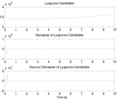
3.5 3.45 3.4 0 5 0 -51 0 0 -2 0 x106 105 Lyapunov Candidate 1 2 3 4 5 6 7

Derivative of Lyapunov Candidate

8 9 10

1 2 3 4 5 6 7 8 9 1

107 Second Derivative of Lyapunov Candidate

1 2 3 4 5 6 7 8 9 1

Time [s]

Figure 10 - Lyapunov candidate and its time derivatives plotted for the stable simulation. Note how the first time derivative is always negative, and that V(x) tends towards a finite limit.

4

3

0 1 2 3 4 5 6 7 8 9 10

X 106 Derivatie of Lyapunov Candidate

1 1 11

0

0

x

1 2 3 4 5 6 7 8 9 10

Second Derivative of Lyapunov Candidate

-2 1 1 1 1 1 1 1 I

0 1 2 3 4 5 6 7 8 9 10

Time [s]

Figure 11 - Lyapunov candidate and its time derivatives plotted for the unstable simulation. Note how the time derivative of V(x) becomes positive at several points (one is marked in the figure).

As is shown in these plots, the stability of the system can be determined by applying Barbalat's lemma to the Lyapunov candidate computed using SOSTOOLS. For the stable case, V(x) is invariably positive definite, as the algorithm searches through only positive definite functions for one with a negative definite time derivative. In addition, since V(x) is always less than zero (as shown in Figure 10), V(x) tends towards a finite limit. Lastly, V(x) is uniformly continuous, as seen in both the plot of

V(x), which is bounded. In addition, this can be seen in the fact that V(x) is merely a function of the state, which is bounded because V(x) tends towards a finite limit, and is a function of the state as well. V(x) can be shown to be bounded through this same logic, and as such proves again the uniform continuity of V(x). Therefore, V(x) -+0 as

t -+ oo. This in turn implies that the state goes to its desired point, since V(x) =0 at this

point. The equation for V(x), shown in full in Appendix 4, verifies that V(x) =0 at the desired point. However this is also seen in the fact that V(x) is defined as such:

. ... . ... ..... . ... ... -.. .-.-.. .. ... -,

--X 106 Lyapunov Candidate

) V . (86)

ax

In order for V(x) to equal zero, i must equal zero. This means that the system will converge to the fixed point, which is the desired state. For the unstable case, V(x) does not remain less than zero, and as such the system V(x) does not converge to zero. Therefore, this function is an indicator of stability, as long as V(x) < 0.

Using this simple metric, the region of attraction of this controller was calculated.

By iterating through initial condition, and simulating the system, one can calculate the

values of V(x) for the simulation. If V(x) <0 for this finite time, it can be reasonably concluded that the system is stable. This was done for initial conditions in a, 9,

a,

Figure 12 -Region of attraction based on analysis of a Lyapunov candidate function at varying initial conditions for a and d. Note that the white region corresponds to the attractive region. In addition the bounds on a are the initial conditions in which the beam starts contacting the left and right edges of the cylinder.

-10 - d

-1.5 -1 -0.5 0 0.5 1 1.5

Theta [rad]

Figure 13 -Region of attraction based on analysis of a Lyapunov candidate function at varying initial conditions for 0 and 9. Note that the white region corresponds to the attractive region. In addition, the bounds on 9 are the initial conditions in which the beam starts contacting the left and right edges of the cylinder.

0.25 0.2 0.15 0.1 0.05

0

-0.05

-0.1

Figure 14 -Region of attraction based on analysis of a Lyapunov candidate function at varying initial conditions for a and do. Note that the white region corresponds to the attractive region. In

addition, the bounds on a are the initial conditions in which the beam starts contacting the left and right edges of the cylinder. In addition, be aware that varying values in do must use different Lyapunov candidate function, since the dynamics are changed when do is varied

These regions are "slices" of state space, and the region of attraction has a ninth-dimensional shape. The regions correspond to when the other states are at the desired point, and the states displayed are varied. This allows for this region of attraction to be

more plainly seen.

As seen in these figures, the region of attraction is a relatively broad one. Unfortunately, this is done with unrealistically high control inputs on the order of 5000 N-m (see Figure 8). The following section will be concerned with designing a controller than not only reduces the required torque to stabilize the system, but also increases the region of attraction as much as possible.

LQR Trees

The controller detailed previously is able to stabilize the system locally. It has a relatively large region of attraction, yet this can be improved upon. This can be done by applying the LQR Trees algorithm. This algorithm creates a controller that is in actuality a series of locally stable LQR controllers. Each controller is able to coerce trajectories to the region of attraction of the another controller, which passes the trajectory to another region of attraction for another controller, and so on until the trajectory reaches the desired point in state space. The controller exists in a "tree" of these controllers in which any initial point in state space (within a certain range) will follow a chain of controllers to the desired point. For simplicity, no adaptation principles were used when the LQR trees

algorithm was applied to the cylinder-beam system.

An additional advantage of using this algorithm is that the linear controllers will require much lower control inputs. The nonlinear adaptive controller has somewhat unrealistic torque requirements (on the order of approximately 5000 N-m). Therefore,

another advantage of applying this algorithm is to have much more reasonable torque requirements.

The LQR trees algorithm begins with the controller that is applied last during simulation of the controller. Specifically, this is the LQR controller about the desired point. The tree of controllers terminates at this point, and for this reason it is the "final"

controller. To design the controller, the system was first linearized about the desired fixed point:

dafx) X+ _afx)

Iax lx=xd,,i,,,u=0 au x=xd.,,,d ,u=0

u=Ax+Bu (87)

Using this linearization, the following LQR gain matrix was found using the cost matrices

Q

K =[-1.9192 1.6036 -0.8977 2.1128] (88)

In order to determine the region of attraction for this controller, the invariant set theorem can be applied. The invariant set theorem states [5]:

If:

-For I>0, V(x) is bounded in the region Q, defined by V(x) < 1

-V(x) <0 for all x in Q,

Then V(x) -> 0 as t -> oo.

Therefore, we must find a Lyapunov candidate for which in some region this is true. A suitable candidate is the cost function associated with the LQR controller:

V=xTSx >O0

Y

=2x

(89)

(90)

A region must be found in which the invariant set theorem can be applied. Therefore, a

search for the level set 1 must be done. This can be carried out using an S-procedure, which is done computationally using a sums-of-squares program. The S-procedure

essentially is a search for the maximum 1 with which the following polynomials are positive definite[8]:

-#+A(x)(V -l) >0

A(x)

>0

If this is true, then the conditions of the invariant set theorem are met for the region (91)

(92)

defined by V(x) < 1 (i.e.

V(x)

1=0.6738

(93)

This domain of attraction is shown visually in the following figures:

0.8- 0.6- 0.4- 0.2- 0- -0.2- -0.4- -0.6- -0.8-1 1.2 1.4 1.6 1.8 2 Alpha [rad] 2.2 2.4 2.6 2.8 3

Figure 15 - Region of attraction of the time invariant LQR controller seen in the a, d plane. The bold ellipse shows the outline of the region, and the thin lines are sample trajectories initialized on the edge of the region in order to demonstrate the stability of the system in this region.

--- 0.6- 0.4- 0.2-Co _{-0 -} C -o 0.2 - -0.4--0.6 -0.8 -2.2 -2.15 -2.1 -2.05 -2 -1.95 -1.9 -1.85 -1.8 Theta [rad]

Figure 16 -Region of attraction of the time invariant LQR controller seen in the 9, 9 plane. The bold ellipse shows the outline of the region, and the thin lines are sample trajectories initialized on the edge of the region in order to demonstrate the stability of the system in this region.

This provides us with a region in which this controller can be stably applied.

Growing the Tree

The next step is to create some nominal trajectories leading to this region from random points. Random points are chosen because of the fact that, much like a Rapidly Expanding Random Tree (RRT) algorithm, guarantees can be made stating that as t -+ oo

the entire state space will be filled by the tree [8].

Of course, a choice must be made as to limits of these random points. Because of

the physical constraints of the system, this choice is relatively simple. Due to the fact that the dynamics make little sense when the beam is on the bottom of the cylinder, the random points must ensure that the beam begins in contact with the cylinder on some point on top of the cylinder. In addition, 9 must be within a range such that the contact point is on the length of the beam. These constraints were tightened slightly in order to

. ... ..... ..... . .. ... .... ... ... ...

prevent failures in the trajectory optimization algorithm. The final conditions correspond to the following constraints:

(94) --

<a+6<-2

2

-4< 0 <0 (95)

The choice of the limits of the initial velocities of the system

(a

-1<0<1 (96)

-1<a<1 (97)

The nominal trajectories from these random points to a point on the existing tree represent new branches in the LQR tree. In order to add new branches to the tree, we must stabilize the trajectories using time-varying LQR controllers, and then determine the regions of stability of the controllers using similar analysis as that for the time invariant case seen above. This allows us to determine exactly which regions in state space are "covered" by the tree. As this "tree" grows, the trajectories may also terminate at points in previous nominal trajectories, depending on what point is closer from a distance metric based on the potential function seen in equation (89). This can be repeated until the regions of stability for all of the controllers combine to cover a suitable large portion of the state space.

In order to generate nominal trajectories, well established shooting methods were used in order to minimize the cost function [1]:

In this, xf is the final point in the trajectory, xde,, is the desired endpoint for the trajectory,

and Qf is a weighting cost matrix (set to be identity). Minimizing this cost function places the end of the trajectory as close as possible to the desired endpoint. This

minimization was done using the Sequential Quadratic Programming (SQP) toolbox for MATLAB, SNOPT [2]. Gradients of the cost function were calculated using Back Propagation Through Time (BPTT). An example of this trajectory optimization for a random state can be seen in the following figures:

0.5 F

I I I I I I

Random State Desired State

10

1.55 1.6 1.65 1.7 1.75 1.8

Alpha [rad]

1.85 1.9 1.95 2

Figure 17 -Example of trajectory optimization for random initial conditions seen in the a, a plane U)

<0

-0.5

I I f - -- - r- - -- 4- -- - ' ) I

-2.4 -2.3 -2.2 -2.1

Theta [rad]

-2 -1.9 -1.8

Figure 18 - Example of trajectory optimization for random initial conditions seen in the 9, 9 plane

The Time-Varying LQR Controller

Once a nominal trajectory is found, it must be stabilized using a time-varying LQR controller which coerces nearby trajectories to this trajectory. A time-varying LQR controller can be made by first linearizing the dynamics about the nominal trajectory generated previously: X(t) = x(t) - x0 (t) _i(t) = u(t) - u0 (t) x ~ A(t)xY(t) + B(t)ii(t) (99) (100) (101)

Where x0 (t) and u0 (t) are the nominal trajectories. As with the time invariant LQR

controller, a cost function must is used with the form: Desired State Random State -1 I -2.5 ... . ... -0.5

J = Y(t f) QfX(tf )+

tf

f[ [(t)

Q(t)

+

0

Where

Qf

Q,

J= X(t)

_{S(t)i (t)}

The following Riccati Equation is found, which S(t) is a solution for:

S(t)

S (104)

This can be solved by integrating backwards in time, in order to preserve the boundary condition:

S(tf )=

_Qf

The solution calculated for S(t) leads to the following optimal feedback control law:

(106)

This feedback law will stabilize trajectories to this nominal trajectory, given the

trajectory is initialized within the region of attraction of the controller. The values used for the cost matrices Q , R, and

Qf

(102)