Coordinated Jacobian transpose control and its application to a climbing machine

Coordinated Jacobian Transpose Control

and its Application to a Climbing Machine

by

Craig Daniel Sunada

Bachelor of Science in Mechanical Engineering University of Colorado, Boulder (1992)

Submitted to the

Department of Mechanical Engineering

in partial fulfillment of the requirements for the degree of

Master of Science in Mechanical Engineering

at the

Massachusetts Institute of Technology

August 1994

© 1994 Massachusetts Institute of Technology

Signature of Author

Department of Mechanical Engineering August 21, 1994 Certified by // V, _--_!_ / _{Steven Dubowsky} Thesis Supervisor Accepted by -Ain A. Sonin Chairman, Departmental Graduate Committee

Raotw %

MASSACHUSETTS INSTITUTE

Coordinated Jacobian Transpose Control

and its Application to a Climbing Machine

Submitted to the

Department of Mechanical Engineering

in partial fulfillment of the requirements for the degree of Master of Science in Mechanical Engineering

by

Craig Daniel Sunada

Abstract

This thesis proposes a control algorithm based on Jacobian Transpose Control for coordinated position and force control of autonomous multilimbed mobile robotic systems performing both mobility and manipulation. The technique is called Coordinated Jacobian Transpose Control, or CJTC. CJTC has advantages over other techniques used to control multilimbed mobile robots, including being computationally inexpensive and providing a simple and unified interface with higher level planners. It can also control functions other than positions and orientations of the system. A methodology called the Extended Mobility Analysis is presented to choose a set of control variables that does not overconstrain the system. The effectiveness of CJTC is demonstrated in laboratory experiments on a climbing system.

Thesis Supervisor: Dr. Steven Dubowsky

Acknowledgments

Betsy, my love, thank you for your love, your support, and your understanding. I never dreamed that love could be so overwhelming before we met. Alex, even though you are still too young to understand what I say, thank you for being such a wonderful son. I am ever so grateful that you are much better behaved than I was at your age. Thank you also for reminding me just how small my work is compared to the miracles that surround me every day.

To my parents, who provided the guidance and inspiration that led me to MIT, this thesis is proof of your accomplishments as parents and teachers of me. I hope that I can do as well for my son. To my brother Wade: our rivalry helped spur me to greater

heights than I would have achieved alone.

To the rest of my family: Glen, Aunt Dorothy, Aunt Grace, Granny, Aunt Tania, and all the others, thank you for your support. The strong foundation of the love that my family shares allowed me to reach these levels.

Rick and Lucy, thank you for your support. Even though I have only known you for two years, you are already family in my heart. Hopey, even though you will never comprehend anything, you still give me your unconditional love.

Bob and Fran, thank you for your hospitality. You have made me feel welcome in this strange, hostile city. Sophie and Hannah, I hope that you also strive for educational excellence, and that in some small way I helped inspire you.

Dr. Dubowsky, thank you for providing me with insight and guidance in much more than just academics and research. Someday I will tell my students your stories (or stories about you).

Tom, thank you for your friendship, as well as your technical help. I would like to thank Dalila Argaez for her contribution to my work: she started it all! I would like to thank my fellow students for their assistance during my research: Jeff Cole, Nathan Rutman, Richard Wang, Michelle Tescuiba, and Pengyun (Perry) Gu. I hope to see you all at my next barbeque! Joe Deck, thanks for imparting upon me some of your perspective on life at MIT.

The support of this work by NASA (Langley Research Center, Automation Branch) under Grant NAG-1-801 is acknowledged.

Table of Contents

Abstract ... 2 Acknowledgments ... 3 Table of Contents ... 4 List of Figures ... 5 Nomenclature: ... 6 1: Introduction ... 7

1.1: Purpose and Contributions ... ... 7

1.2: M otivation ... 8

1.3: Background ... 10

1.3.1: Existing M ultilimbed M obile Robots ... . 10

1.3.2: Control algorithms ... ... 12

1.4: Assumptions... 16

2: Control Scheme Development ... 19

2.1: Jacobian Transpose Control ... 19

2.1.1: Derivation of Jacobian Transpose Control ... 21

2.2: Coordinated Jacobian Transpose Control ... 22

2.2.1: Derivation of Coordinated Jacobian Transpose Control ... 23

3: Control Vector Selection... 26

3.1: Control Variables ... ... 26

3.2: Control Vector Selection ... ... 27

3.2.1: Gruebler's M obility Analysis ... .... .28

3.2.2: Extended M obility Analysis ... 31

4: Application of CJTC to a laboratory climbing robot ... 39

4.1: System description ... 39

4.1.1: Climbing M achine ... ... ... 40

4.1.2: Power Amplifiers ... 43

4.1.3: Control Computers ... 43

4.2: Climbing Gait... 44

4.3: Control Vector Selection... ... 45

4.4: Control equations ... 51

4.5: Control gain selection ... 53

4.5.1: Dynamic M odel ... 53

4.6: Experimental performance ... ... 57

4.6.1: Data from climbing stage one ... 57

4.6.2: Data from a full climbing cycle ... 61

5: Summary and Conclusions ... 67

6: References ... 68

Appendix A: LIBRA Jacobian Equations ... 73

Appendix B: Power Amplifiers... 77

Appendix C: Gain Selection ... ... 84

List of Figures

Fig. 1: A Schematic of the LIBRA climbing system ... 8

Fig. 2: A multilimbed mobile robot ... 9

Fig. 3: A representative multilimbed mobile robot ... 18

Fig. 4: Block Diagram of Jacobian Transpose Control ... 20

Fig. 5: 2-link manipulator controlled through JTC ... . 20

Fig. 6: Multilimbed Mobile Robotic system controlled through CJTC... 23

Fig. 7: Block Diagram of CJTC ... ... 24

Fig. 8: Common Planar Constraints ... ... 30

Fig. 9: Stage One of the Extended Mobility Analysis ... 33

Fig. 10: Stage two of the Extended Mobility Analysis ... 35

Fig. 11: Over actuated system ... 36

Fig. 12: Over actuated system with environmental and internal constraints relaxed ... 36

Fig. 13: The LIBRA climbing system... ... 39

Fig. 14: LIBRA system block diagram ... ... 40

Fig. 15: A Schematic of the LIBRA ... ... 41

Fig. 16: Climbing Gait used by the LIBRA ... 44

Fig. 17: LIBRA under full environmental constraints ... 45

Fig. 18: Constraining x of the Center Body ... ... 46

Fig. 19: Constraining x,y of the Center Body ... 46

Fig. 20: Constraining x,y,0 of the Center Body ... 47

Fig. 21: Constraining x,y of Foot 3 ... ... 47

Fig. 22: Relaxing the x environmental constraint ... 48

Fig. 23: LIBRA with control vector 1 ... ... 49

Fig. 24: LIBRA with control vector 2... ... 50

Fig. 25: LIBRA with control vector 3 ... 51

Fig. 26: Model of the LIBRA top kinematic chain ... 54

Fig. 27: Dominant poles of the LIBRA for ybody from -0.20m -> 0.14 m... 56

Fig. 28: Desired motion for the climbing robot ... 58

Fig. 29: xb, Yb position for a pushup maneuver ... 59

Fig. 30: Ob for a pushup maneuver... .... ... 59

Fig. 31: x2 Force for a pushup maneuver... ... 60

Fig. 32: x3 location for a pushup maneuver ... ... 60

Fig. 33: Desired Cartesian movements for one gait cycle ... 61

Fig. 34: Actual Cartesian movements for one gait cycle ... 62

Fig. 35: Body movements for one gait cycle ... ... 63

Fig. 36: Body orientations for one gait cycle ... ... 63

Fig. 37: x positions for all the feet for one gait cycle ... .64

Fig. 38: y positions for all the feet for one gait cycle ... 64

Fig. 39: Foot 1 position vs. time for one gait cycle ... .65

Fig. 40: Foot 2 position vs. time for one gait cycle ... .65

Fig. 41: Foot 3 position vs. time for one gait cycle ... .66

Fig. B 1: Power amplifier schematic ... 78

Fig. B2: Power Amplifier Card Layout ... ... 79

Fig. Cl: Model of the LIBRA ... ... 84

Fig. C2: Poles of the LIBRA for ybody from -0.20m -> 0. 14m ... 93

Fig. C3: Dominant poles of the LIBRA for ybody from -0.20m -> 0.14 m ... 94

Fig. C4: Bode plot for the xbody position variable... 95

Fig. C5: Bode plot for the ybody position variable... 96

Nomenclature:

a = number of DOF of a system under full environmental constraints b = number of uncontrolled DOF of a system under the current constraints F = number of DOF of a system using Gruebler's mobility analysis

F = vector of desired forces fl = number of slider or pin joints f2 = number of roll-slide joints fi = number of DOF of joint i G(q) = gravity compensation vector

j

= number of joints of a system Ji = joint i

p = proportional gain matrix = derivative gain matrix 1 = number of links of a system mi = number of active joints in limb i n = number of limbs

r = number of control variables in the control vector s = total number of active joints

t = input vector of joint efforts u = control vector

Mcmd = commanded position of the control vector x,y,z = Cartesian coordinates

1: Introduction

1.1: Purpose and Contributions

The purpose of this thesis is to develop a control technique that can control both mobility and manipulation of a multilimbed mobile robot while being computationally feasible for small on-board computers. Mobility refers to the locomotion of the robot, whether through walking, climbing, sliding, or other forms of limbed locomotion, and manipulation refers to the interaction forces exerted on a task and the manipulation of an object in the environment. Here, an approach called Coordinated Jacobian Transpose

Control, or CJTC, is proposed for the control of multilimbed, multi-degree of freedom mobile robotic systems. An extension of classical Jacobian Transpose Control, CJTC uses the simplest form of impedance control and an extended Jacobian matrix to control the entire system's forces and motions in a consistent and coordinated manner while being computationally feasible for small on-board computers. The effectiveness of CJTC is demonstrated in laboratory experiments on a three-limbed climbing system called the Limbed Intelligent Basic Robotic Ascender, or LIBRA, shown schematically in Figure 1. This system was designed and built by Dalila Argaez, and she first proposes the concept of CJTC 1. This thesis develops her concept into a working control scheme and demonstrates its effectiveness. This first chapter presents the motivation for studying multilimbed mobile robots, and the need for new control algorithms to control

Fig. 1: A Schematic of the LIBRA climbing system

1.2: Motivation

The area of multilimbed mobile robots is an expanding field, with many important applications. It is becoming increasingly clear that multilimbed mobile robots are going to be important for performing tasks in areas that are either inaccessible to humans or undesirable or unsafe for humans to work. Such applications include toxic waste handling and work at nuclear sites 2, 3, 4, 5, 6, 7. Multilimbed mobile robots are virtually

the only feasible solution for planetary exploration 8, 9, 10. These tasks take place in partially structured environments, where the general characteristics and layout of the terrain and tasks are known, but the specific details are not. Most of these tasks require

the robot to interact with the environment -- taking measurements and manipulating objects. Manipulation tasks may require carefully controlled forces to be applied. Often, the manipulation tasks will have to be performed while also moving the robot. For instance, a mechanical monkey might scurry into a toxic waste area and carefully take some measurements. Another part of its task might be to then shut off a valve, and then pick up a waste drum and carry it out. An example of a multilimbed robotics system is shown schematically in Figure 2, with limbs that are capable of both mobility and manipulation. As discussed in the next section, no multilimbed mobile robotic system in existence today is capable of performing tasks requiring both mobility and manipulation simultaneously, and that new control algorithms need to be developed to perform such tasks.

aition

Fig. 2: A multilimbed mobile robot

TT ~~ rr r I·~~·L·~H· ~~+~1

---1.3: Background

1.3.1: Existing Multilimbed Mobile Robots

Multilimbed mobile robots in existence today are a wonderfully diverse set of machines, ranging from pogo-stick like hopping machines " to mouse-like miniature walking machines 12 to massive walking vehicles 13. The types of mobility displayed by these robots can be classified into two separate categories: dynamically and statically stable. Dynamic movement relies on the dynamics of the system for mobility and stability. Raibert's hopping machines 11 and Fukuda's brachiation machine 14 are examples of this type of movement. While effective and potentially faster over smooth or well-known terrain, these machines are generally not suitable for the rough, partially structured terrains that would be found in the tasks described above. Statically stable machines are more effective for these tasks, and are the focus of this thesis.

Statically stable movement refers to the notion that if the robot were to freeze at any point in its movement, then it would not fall over. The number of robots that use this type of movement is quite large. Dante and Ambler are two well-known walking machines used to study potential systems for planetary exploration 15, 16. Planetary exploration requires legged locomotion to handle the extreme terrains that are encountered. The Adaptive Suspension Yehicle, or ASV, built at Ohio State University as a proof-of-concept vehicle is a massive 5.8 m long six-legged walking vehicle 13, 17. It has demonstrated the feasibility of walking as a viable form of locomotion on a large scale. Many smaller hexapod walking machines have been built, including the Moscow State Hexapod 18, the OSU Hexapod 19, and the CMU Hexapod 20, as well as some very small hexapods such as Genghis and Atilla built by Brooks 12, 21. These have mainly been used to research the control and planning issues involved in walking. Other forms of walking machines have also been built, such as the NCTU Quadruped22. Hirose 23

built Titan III, a quadruped that is capable of both statically stable and dynamic walking. Multilimbed mobile robotic systems used for climbing include the Portsmouth Polytechnic Robug II, which uses vacuum grippers to climb walls 24. Neubauer 25 built a 6 legged climbing machine that uses friction to climb between two walls. Gradetsky et. al. 26 discuss a climbing robot using vacuum grippers for actuation. Hirose 27 has also built a climbing machine with vacuum grippers, capable of both statically stable and dynamic walking. While these walking and climbing machines have demonstrated substantial capabilities, none of these systems are capable of manipulation.

While mobility is certainly the first step in field robotic systems, manipulation must also be addressed. Even the field robots such as Dante aren't capable of manipulation, but rather are used simply to position sensors. The ability to collect ground samples, move obstacles, and probe the environment would all enhance the utility of Dante as a terrestrial exploration robot. One robot that is capable of both mobility and manipulation is the Savannah River Nuclear Mobile Robot -- a hexapod robot with a manipulator mounted on top 28. However, during manipulation tasks the base is usually stationary and it is not capable of controlling both mobility and manipulation simultaneously. Despite this significant drawback, it has been found to be useful enough to warrant a second generation of the design. There are also a number of mobile robots that use tracks or wheels for mobility rather than limbs have been built and used that are capable of manipulation and have proven to be quite useful. HAZBOT, for instance, is used for hazardous materials handling 7, and the Foster Miller Ferret has proven to be very effective in explosives handling 29.

While the current designs of multilimbed mobile robots largely ignore manipulation or treat manipulation separately from mobility, given the usefulness of other systems capable of both mobility and manipulation, new multilimbed mobile robots are sure to be

developed that will be capable of simultaneous mobility and manipulation. In order to control these future systems, new control schemes will need to be developed.

1.3.2: Control algorithms

Control algorithms that would allow the control of manipulation forces and motions while simultaneously controlling the trajectory of the rest of the system have yet to be developed for multilimbed mobile robots. The Savanahh River Nuclear Robot, a current experimental multilimbed mobile robotic system capable of both mobility and manipulation, treats mobility and manipulation separately -- performing only one or the other at a time. It also does not control the forces exerted on the environment 28. In order to increase the utility of robots, new control approaches must be developed to control simultaneously the motions of such articulated multilimbed mobile robotic systems and the forces that they exert on their environment or tasks. One way to develop new approaches is to attempt to extend the current methods used for mobility to also include manipulation, or to attempt to extend current methods used for manipulation to also include mobility.

A significant amount of work has been done in the area of the control of walking machines. A common form of control currently used is simple joint space position control. However, this form of control cannot directly control the forces being applied to the environment, and therefore isn't applicable for the control of forces during manipulation. Joint space position control also produces rough, jerky motion of the body of the robot in Cartesian space, and is difficult to adapt for rough terrain and changes in the environment 30. A form of force control is therefore required.

A common form of control used that controls the forces being applied to the environment is called coordinated walking. Coordinated walking is an inverse plant controller, and like other forms of inverse plant controllers, coordinated walking is

computationally expensive, requires a detailed model of the system, and is sensitive to modeling errors 31. One form of coordinated walking treats the legs as force servos and resolves the desired motions and a force distribution algorithm into forces to be applied by the legs 32, 33. This type of controller has demonstrated problems associated with practical difficulties in getting the legs to act like high-performance force servos 30. Also, the system performance is low because the bandwidth of the overall trajectory controller must be substantially less than the bandwidth of the legs' controllers 31. Designing this type of coordinated walking is difficult because of the sensitivity to modeling errors. Without incorporating the often difficult to model actuator dynamics in the controller or analysis, the control gains must be chosen by trial and error 31. Another form of coordinated walking includes a simple model of the actuator dynamics in its model of the system, and directly reflects the desired trajectory and limb forces to the limb actuators 31. While this controller offers several advantages, such as the ability to decouple the system and linearize the control, it is also very computationally expensive. The ASV, which uses this control scheme, has 16 dedicated processors for the control alone 13 Coordinated walking does not address the issue of manipulation. Although it might be possible to extend coordinated walking to include manipulation, the computational burden would be large. While this is acceptable on large systems such as the ASV that can carry powerful computers, for small self-contained systems with small capability processors, this would not be feasible. Also, the sensitivity to modeling errors would pose a problem when manipulating an object in a partially known field environment where a detailed model of the object is not available. Given the limitations of that this controller would have, another approach for controlling mobility and manipulation is desired.

Looking for another way to develop a control algorithm to control both mobility and manipulation, control techniques that are currently used for manipulation are examined to see if they could be extended to also control mobility. There are two primary forms of

force control used to control fixed base serial manipulators -- hybrid control and impedance control. Khatib shows how generalized joint torques are reflected at the end-effector for redundant manipulators, an important understanding for either form of force control of redundant manipulators 34. Raibert and Craig propose a hybrid control scheme to control manipulator motions to satisfy position and force constraints simultaneously, and have demonstrated this approach through controlling the end-effector of a two link fixed-based manipulator 35. Hybrid control can also be extended to systems other than simple serial manipulators. For instance, Yoshikawa and Zheng extend hybrid position/force control to multiple robot manipulators working in well-known environments 36. However, hybrid control techniques require detailed knowledge of the environment for effective force control, including a good estimate of the environmental stiffness 37. Since such an estimate probably would not be available in a partially known environment, hybrid control is not suitable for this research.

Impedance control is the other primary form of force control. Hogan introduced impedance control, which controls a relationship between force and displacement, as a unified method for controlling the force and the position of a manipulator's end-effector 38, 39. _{Hogan also asserts that it is possible to superimpose impedances, which is} necessary if multiple degrees of freedom are to be controlled. Schneider and Cannon use Hogan's impedance control approach to arrive at an object impedance controller for cooperative manipulation, which gives a straightforward interface for supervisory control by directly controlling the object being manipulated 40, 41. Impedance control has demonstrated good stability in contact transitions -- a quality than many other force control schemes lack 42. It also does not require precise knowledge of the environment, in contrast to hybrid control. Some simple forms of impedance control don't even require a dynamic model of the system. Given these characteristics, impedance control is promising as a possible controller for both mobility and manipulation.

Current control techniques that deal with mobility and manipulation are investigated for possible methods to extend impedance control to control simultaneous mobility and manipulation. A number of control algorithms have been developed for motion control of manipulators mounted on simple vehicles, such as on spacecraft and trucks 43, 44 Hootsmans and Dubowsky use an extended Jacobian matrix to compensate for base dynamics while using Jacobian Transpose Control to control a manipulator mounted on a mobile base 45. However, these algorithms only look at manipulation while compensating for base movements and do not actively control the base. Seraji, on the other hand, proposes an extended Jacobian matrix to actively control the motions of a system composed of a manipulator mounted on a track or otherwise mobile base through inverse Jacobian control 46, 47. His control algorithm was demonstrated experimentally on a 7 DOF robot arm mounted on a motorized track 48. The use of an extended Jacobian

matrix might allow impedance control to control both mobility and manipulation.

While there currently is no control algorithm reported in the literature that controls both the mobility and manipulation of a multilimbed mobile robot, several promising avenues exist. As discussed before, coordinated walking could be extendible to control manipulation, but would probably be too computationally expensive for this problem. Impedance control, currently used for manipulation with serial arms, is promising for both the ability to control the position of the end-effector while it is free and the forces it exerts while constrained, and for stability during contact transition. The use of an extended Jacobian matrix, similar to Seraji 46, 47 or Hootsmans 45 might enable impedance control to control multiple points on a robot in order to control both manipulation and mobility, and this is the approach pursued in this research.

1.4: Assumptions

The need for developing a new control algorithm that controls both mobility and manipulation has been discussed, but the exact problem domain remains to be defined. The range of systems and tasks that could be covered by the terms 'multilimbed mobile robot' is too large to be covered by any single control scheme, and specific assumptions need to be made to limit that range. Assumptions are made about the nature and requirements of the environments and tasks, the computational capability and the

kinematics of the class of robots to be controlled.

It is assumed that the robot is operating in a partially known environment. This implies that the general nature of the environment is known, and perhaps even the general layout of the environment and task, but the precision to which these things are known beforehand is not great, perhaps to within 5% or 10% of the limb span of the robot. The order of magnitude of the environmental stiffness might be known, and an approximate mass of an object to be manipulated, but detailed models will not be available. This assumption is representative of robots working in field environments, and prevents the use of control schemes that require good knowledge of the environment, such as hybrid control. It also prevents the use of control schemes that require a detailed dynamic model of the task and environment.

It is assumed that the task will require the forces being applied to the task to be controlled, but not to great precision. This assumption is made to allow a control scheme without force feedback. It is also assumed that for all tasks, all degrees of freedom of the system under the full kinematic constraints imposed by the environment must be controlled. This is generally required for acceptable system performance 49.

It is assumed that the computational capability will be from a single processor of medium capability -- approximately the capability of an Intel 80386 processor or a

Motorola 68020. This represents an accessible amount of processing capability for almost any size except for very small systems.

These assumptions are not suitable for every multilimbed mobile robotic system, and limit the applicability of the control scheme developed in this thesis. Also, many of these assumptions are qualitative, and are meant as guidelines. As technology changes and additional sensors, actuators, and computational capability become readily available, many of the assumptions made may be relaxed. For instance, if much more processing capability is readily available, then it might be desirable to develop other control techniques that take advantage of that fact and subsequently give better performance.

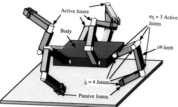
The following is a description of the kinematics of the class of robots to be treated in this thesis. Figure 3 shows an n-limbed mobile robotic system representative of the class of robots dealt with herein. The system contains one main body with the n limbs attached and a base, which represents the ground. Some of the limbs position the main body with respect to ground for mobility purposes, while the remaining limbs may perform manipulation tasks or be free. It is assumed that the ith _{limb is a ji joint serial chain where}

mi of the joints are active and (ji-mi) joints are passive. Among the (ji-mi) passive joints, some are passive due to the physical contact of the limb with the ground or a manipulated object; the others are mechanical non-actuated joints. The total number of active joints for the system is given by:

s= 1mi. (1)

The kinematic variables qi of the s active joints form a set that is referred to as the joint vector g. The effort variables of the system's actuators, a torque for a revolute joint or a force for a prismatic joint, are the inputs to the system; they form the s by 1 input vector :. It is assumed that the actuators are backdrivable.

Active Joints

Fig. 3: A representative multilimbed mobile robot

Active

2: Control Scheme Development

Looking at existing control techniques and given the assumptions made, a form of impedance control is chosen to be extended to control both mobility and manipulation for the following reasons. Given the need to actively control forces, either impedance control or hybrid control could be used. Given the assumption of partially known environments, hybrid control would have been difficult to implement. Impedance control does not require exact knowledge of the environment. Given the restriction on computational capability, the simplest form of impedance control, Jacobian Transpose Control 37??? is used. This control does not require the use of force sensors for feedback, which might be advantageous for some systems. Controlling forces without force feedback is only possible with the use of backdrivable actuators, which is assumed in the previous section.

2.1: Jacobian Transpose Control

Since Coordinated Jacobian Transpose Control is based on Jacobian Transpose Control, this section first gives the derivation for classical Jacobian Transpose Control (JTC). A complete analysis of Jacobian Transpose Control, including a Lyapunov stability analysis, can be found in 37. Conceptually, Jacobian Transpose Control is proportional-derivative control of the position of the end-effector (x) of a serial manipulator in Cartesian space. JTC controls the dynamic relationship between force and position, or the mechanical impedance of the end-effector. The end-effector is pulled towards the commanded end-effector position by a set of virtual springs and dampers. After calculating the vector of desired forces (E) from these virtual springs and dampers, JTC directly transforms them into desired efforts at the actuators (:) through the transpose of the Jacobian matrix J. A block diagram of the controller is shown in Figure

4. Figure 5 shows this concept applied to a simple two link serial manipulator, where the end-effector Cartesian x and y positions are controlled.

Acmd

kmd

x

Fig. 4: Block Diagram of Jacobian Transpose Control Uxcmd

:tor

Fig. 5: 2-link manipulator controlled through JTC

As with other impedance control approaches, when the end-effector is constrained in a direction, a force is applied in that direction, and when the end-effector is unconstrained in a direction, a motion results. A compliant constraint results in both a force and displacement. Impedance control eliminates the need for switching between control structures to control both the position when unconstrained and force when constrained. This allows simple, intuitive control of the system. Jacobian Transpose Control is also robust to parametric uncertainty both in the manipulator itself and in the environment, and does not require a mass model of the manipulator. Although both position and force

control with Jacobian Transpose Control is not as high performance as some other control schemes, it is quite acceptable and demonstrates good contact stability.

2.1.1: Derivation of Jacobian Transpose Control

The vector of Cartesian coordinates x of the end-effector is defined as: x

y z

x = 1 (2)

Y

or a subset thereof, depending on the degrees of freedom the manipulator has. The desired force vector F is defined to be:

F = K,

-[xd

_- x] + Kd " ['.d - ] (3) The gain matrices Kp and Kd determine the response of the system, and are chosen to

satisfy the controller design requirements. The gain matrices are generally chosen to be diagonal, but can be non-diagonal if coupling between end-effector Cartesian coordinates

is desired.

The Jacobian is defined as the transformation between joint space velocities and Cartesian velocities:

ax

ax aq, _{a q}

_07 ..

aq,-(4)

The end-effector velocities are given by:

Applying the principle of virtual work, which relates infinitesimally small amounts of work performed in control space to infinitesimally small amounts of work performed in joint space, the following basic equation is derived:

t = (q). F (6)

Using the principle of control partitioning 50, a term can be added to compensate for the gravity forces acting on the robot; G(q). The torque command then becomes:

S= JT _{(q) F + G(q) (7)}

Combining (3) and (7), the control algorithm becomes:

= jT(q) (K, -[x -X] + Kd.[~md -k])+ G(q) (8)

2.2: Coordinated Jacobian Transpose Control

Coordinated Jacobian Transpose Control extends Jacobian Transpose Control, given in the last section, by using an extended control vector and an extended Jacobian matrix. Rather than just controlling the vector of end-effector positions x, CJTC controls the positions and orientations of multiple points on the system, plus other differential functions of the joints vector q. The possible positions and other functions to be controlled are the control variables of the system, and the vector of the control variables chosen to be controlled through CJTC is the control vector u. The control vector can be given as:

[(q)

u= oX(q) (9)

where:

x(g) = position of a point on the system

Q(_) = orientations of points on the system, and

Iq() = other functions of the joint vector, such as the potential energy

The control vector is chosen based on what is desirable and possible to control, and Section 3 describes a method for choosing an admissible control vector.

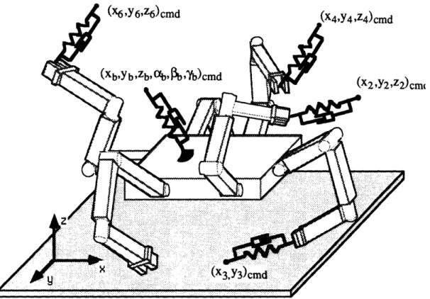
Conceptually, Coordinated Jacobian Transpose Control is proportional-derivative control in control space. Each element of the control vector is forced to move towards its corresponding element of a desired or commanded control vector (Icmd) by a set of virtual springs and dampers in the classical Jacobian Transpose Control approach. Figure 6 shows a multilimbed mobile robot under CJTC with the virtual spring-dampers applied

to the control vector.

) cm

Fig. 6: Multilimbed Mobile Robotic system controlled through CJTC.

2.2.1: Derivation of Coordinated Jacobian Transpose Control

The derivation for CJTC closely follows that of Jacobian Transpose Control, and some

of the same equations will be referenced. A block diagram of the control scheme is given in Figure 7. The additional block for sensors is required if one or more of the control variables are functions of other variables in addition to the joint vector q. In this case, sensors are required that can measure these other variables.

-mcmd

Aýcmd

Sensors Fig. 7: Block Diagram of CJTC

The (rx1) desired force vector E is defined to be:

F= K,

-

[umd - u] + Kd -[ •md - u] (10)

where r is the number of control variables in the control vector

Again, the gain matrices Kp and Kd are generally chosen to be diagonal, and are chosen to satisfy the controller design requirements. Each element of the force vector (F) results in an acceleration of the system if the corresponding element of the control vector (u) is unconstrained or in a force applied to the environment if the corresponding element of the control vector is constrained.

The extended Jacobian is defined as the transformation between joint space velocities and control space velocities:

au_{1 au1}

aqq

...

aq,

aur _aur aqý" _aq.

Bu._.

_Bu...z

•qu

3u

ax, ax,

d-II

aq.

d ... qs

The Jacobian is r by s, where r 5 s is the number of control variables and s is the total number of active joints. The Jacobian does not need to be square, and some redundancies

(11)

can be left uncontrolled if they are not important for the system performance. Combining (7), (10) and (11), the control algorithm becomes:

T = J (q) -(K

-

[ucmd - u] + K,

-

[md - u_) + G(q) (12) Coordinated Jacobian Transpose Control for multilimbed systems has the same advantages that Jacobian Transpose Control offers for serial manipulators. Namely, only the forward kinematics and their derivatives are required, implying a relatively small number of computations. No inertial model of the robot is required. Also, the Jacobian matrix can be rectangular, which is of great importance for redundant systems. CJTC is also robust to parametric uncertainties in both the robot itself and in the environment. Finally, this control scheme provides an intuitively simple interface for controlling end-point positions and forces of a multilimbed system. By moving the commanded endpoints through space or into an object, the limb moves or pushes accordingly. By controlling all the control variables in this fashion, straightforward integration is achieved with higher level planning algorithms.

However, CJTC does not compensate for the changing dynamics of the system, and as a result the performance is configuration dependent. The extent of the configuration dependence is a function of the mass distribution of the robot. When selecting the gain matrices, the controller must be designed for the worst-case configuration 51. If the dynamic response varies dramatically, then performance will be sacrificed significantly over the majority of the workspace. If this is the case, gain scheduling or other forms of adaptation might be required. Also, no attempt is made to decouple the system, and significant coupling between control variables can occur. This can be compensated for by using a non-diagonal gain matrix, but the degree of coupling is configuration dependent and adaptive control or gains scheduling might be required. Despite these characteristics, it will be demonstrated that the control system performance is quite

3: Control Vector Selection

The control algorithm derived in the previous section operates on the control vector u,. and the method for choosing the control vector is presented in this section. The control vector is chosen by the designer, based on the task and the environmental constraints. CJTC allows considerable freedom in choosing the control vector, and this allows the designer to directly control the control variables of interest. The points made in this section are based on general control theory, but are tailored specifically for the CJTC, with all the assumptions and restrictions given in Section 1.4.

3.1: Control Variables

Any differentiable mathematical function of g with non-zero first partial derivatives with respect to q that describes a physical property of the system is defined to be a

control variable. For instance, the Cartesian coordinates x, y and z of a point on the

system are functions of q and are three possible control variables. The Cartesian orientations a, 13, and y of a point on the system are also possible control variables. The most basic control variables are the joint displacements. More abstract control variables might include the system's potential energy or a static stability function to prevent the robot from tipping over. For any given system, there are an infinite number of possible control variables. Of these possible control variables, an admissible set must be chosen to control. A methodology called the Extended Mobility Analysis for choosing an admissible set of control variables is described below. The set of chosen control variables is called the control vector u. The space of control vectors corresponding to all possible configurations of the system is called the control space.

In order to reflect the control errors to the actuators through the Jacobian matrix, the control variables must be written in terms of the joint vector _q. In order to do so, the control variables will generally be written using the assumed environmental constraints both implicitly and explicitly. Since the control variables are functions of the joint vector g, joint position sensors are needed for joint vector feedback. If the control variables are also functions of other variables, then sensors that can measure those variables are also required. Additional sensors might be required to obtain the initial position, to check the position during the movement and correct for errors caused by unexpected slipping, but are not required by the control scheme.

3.2: Control Vector Selection

Choosing the control vector n is not trivial. While the joint vector g is imposed on the system by the mechanical design, the control vector u is chosen by the designer. The designer must choose an admissible set from the infinite number of possible control variables, based on the tasks a specific system must perform, the environmental constraints placed on the system, and desirable performance characteristics. Since the range of possible control variables is so diverse, it is often possible to directly control the points or functions of interest. For instance, if visual feedback from a camera mounted on the robot is important, then good choices for control variables would be the positions and orientations of the camera. If the location of the center of mass of the body is more important, then it is possible to directly control that as well. As stated in the problem definition, all the degrees of freedom of a system under the full kinematic constraints imposed by the environment must be controlled. The environmental interaction forces or other control variables do not have to be controlled, but it often is desirable to do so.

It is important to note that the control vector will change during a robot's mission, based on the changing constraints and desired tasks that the robot will perform. For mobility, it is necessary to lift and maneuver a foot at certain times in the gait, and use that foot to support the body at others. So, for the different tasks and constraints, different control vectors must be chosen. Given the constraints that the system will be subject to, an Extended Mobility Analysis can be performed to determine admissible control vectors.

For the s active joints of the system, s control variables are possible to control. At the lowest level, the s individual active joint positions can be controlled. However, it is not necessary to control all s possible control variables. Sometimes, after choosing a number of important control variables to control, the only control variables admissible to complete the control vector are unimportant for the system. In such cases, it might be wise not to waste the computing resources needed to control these unimportant control variables. When deciding whether to control these unimportant control variables, the designer should consider just how important the control variables are to the system, and how much computing capability is available.

3.2.1: Gruebler's Mobility Analysis

A brief summary of Gruebler's Mobility analysis is given here for review, since it is heavily relied upon in the Extended Mobility Analysis. In this thesis, the term 'mobility analysis' refers to Gruebler's Mobility Analysis. This review is not complete, and a more complete description of Gruebler's Mobility Analysis is given in 52.

An unconstrained rigid body in spatial motion has six degrees of freedom, the x, y, z translations and the a,

J3

and y rotations. A mechanism constructed of I rigid links will

have 6-1 degrees of freedom before they are connected to form a system of links. The connections constrain the system and result in losses of degrees of freedom of the system. Different forms of connectors constrain various numbers of degrees of freedom. A pin joint, one type of lower-pair connector, constrains the three translational degrees of freedom and permits only rotation in one direction. For instance, a link connected to ground through a pin joint has but one degree of freedom, and therefore lost five of the six degrees of freedom it had when unconstrained. A slider joint, another type of lower-pair connector, also constrains five degrees of freedom, as it only allows movement in one translational direction. Another type of constraint is referred to as the roll-slide contact. Two bodies are in contact, but can translate across each others' surfaces and also rotate with respect to each other. Only one degree of freedom -- translation in the normal direction to the surfaces -- is constrained.

Gruebler's equation is now given as:

F = 6.(1-j-1) + Jfi (13)

where:

F = the number of degrees of freedom of the system 1 = the number of links, including the ground j = the number of joints, including ground contacts

fi = the number of degrees of freedom allowed by joint i

In planar motion, there are only three degrees of freedom -- the x and y translations and the single rotation 0. Gruebler's equation in planar motion is given as:

F = 3.(1-1) - 2.fl - f2 (14)

where:

fl = the number of slider or pin joints f2 = the number of roll-slide contacts

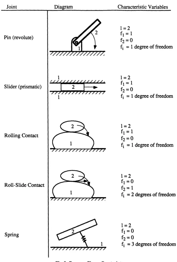
Figure 8, adapted from Sandor and Erdman 53, gives some common planar kinematic joints and their appropriate degrees of freedom.

Diagram Characteristic Variables

Pin (revolute) Slider (prismatic) Rolling Contact Roll-Slide Contact Spring 1=2 f= 1

f2=0

fi = 1 1 2 ZZ 777117777 12 2 1 1=2 fl= 1 f2=0

fi

=

1

degree of freedom degree of freedom 1=2 fl=1 f2=0 fi = 1 degree of freedom 1=2 fl =0 f2= 1 fi = 2 degrees of freedom 1=2 fl=0

f2=0

fi = 3 degrees of freedom

Fig. 8: Common Planar Constraints

Joint

2

3.2.2: Extended Mobility Analysis

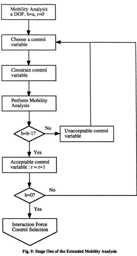
The Extended Mobility Analysis is based on Gruebler's mobility analysis. It addresses which sets of control variables can be controlled for a system subject to a given set of environmental constraints. It also insures that the control variables chosen are independent, and that the system does not become overconstrained. The basic procedure is to repeatedly perform Gruebler's mobility analysis, adding constraints for the control variables chosen and relaxing environmental constraints to test if an interaction force or moment can be controlled. A flow graph of the Extended Mobility Analysis is given in Figures 9 and 10. The nomenclature used is:

a = number of DOF of the system under the full environmental constraints b = number of uncontrolled DOF

r = number of control variables selected s = number of active joints

The first stage of the Extended Mobility Analysis, shown in Figure 9, deals with choosing control variables to control the available degrees of freedom under the full environmental constraints. Performing a mobility analysis on a multilimbed mobile robot under the full constraints of the environment will yield (a) degrees of freedom (b=a). It is assumed all of these degrees of freedom must be controlled for acceptable system performance. If there are less active joints than degrees of freedom (s<a), then the system is under actuated and cannot be controlled using this control scheme. To test if a control variable is admissible, a constraint must be placed on it and another mobility analysis run. If the mobility analysis yields the loss of one degree of freedom (b=b- 1), then the control variable does not overconstrain the system and is admissible. If the mobility analysis does not yield the loss of one degree of freedom (b=b), then the control variable cannot be controlled because it is already constrained by the given environmental constraints or the constraints from the previous control variables chosen. If it is highly desirable to control that control variable, then it is still possible to do so either by choosing it later in

the analysis as a controlled environmental interaction force, if an environmental constraint is constraining it, or by eliminating one or more previously selected control variables, if the control variable constraints are constraining it. If the control variable is inadmissible and it is not highly desirable to control it, then the constraint is removed and another control variable tested. After (a) admissible control variables are chosen and constrained, then the system shouldn't have any degrees of freedom (b--O). If it does, then the set of a control variables chosen are not independent of each other and cannot be controlled simultaneously. If the number of active joints is greater than the number of degrees of freedom (s>a), then it is possible to control a number (s-a) of interaction forces with the environment, internal forces, or other control variables. The second stage of the Extended Mobility Analysis must then be performed.

Mobility Analysis a DOF, b=a, r--O

Yes Acceptable control variable : r = r+1

Interaction Force Control Selection

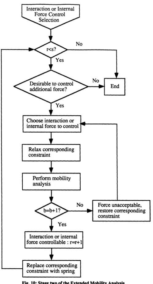
The second stage of the Extended Mobility Analysis, shown in Figure 10, deals with controlling environmental interaction forces and internal forces. At the start of the second stage, all degrees of freedom of the system are controlled, and b=O. To test if a desired interaction or internal force or moment is controllable, a control variable is chosen as the desired interaction force with the environment or internal force, and the environmental position constraint or internal displacement constraint on that control variable is relaxed. With all the other control variables constrained, the system should then have one additional degree of freedom (b=b+1). If so, then that force or moment is controllable. To mark that the force or moment is controlled, replace the corresponding constraint with a spring. Note that a spring does not act as a link or constraint for purposes of a mobility analysis and it is merely there to indicate visually that the corresponding interaction force is being controlled. If the system does not have an additional degree of freedom (b=b), then that interaction or internal force is not controllable, perhaps due to the other control variables chosen or because the mechanism cannot apply forces in that direction. In this case, restore the original constraint. If there are still more actuators than control variables chosen (s>r), then additional control variables can be controlled, if desired.

Desirable to control additional force?

Choose interaction or internal force to control

Force unacceptable, restore corresponding constraint

Interaction or internal force controllable : r--r+1

Fig. 10: Stage two of the Extended Mobility Analysis

Replace corresponding constraint with spring

It is possible that all controllable environmental interaction forces are controlled before r=s, and the only additional control variables that can be controlled are the internal forces. Such a system is shown in Figure 11. The system has zero degrees of freedom with all environmental constraints in place. After relaxing an environmental constraint in the x direction, the system has one degree of freedom, and therefore the environmental interaction force can be controlled. However, r = 1, s = 2, therefore r<s, so an additional control variable can be selected. Relaxing an internal constraint on prismatic actuator 2 yields an additional degree of freedom, and thus an internal force can be controlled as well as the environmental interaction force, as shown in Figure 12. However, this force might not be important and the designer might very well elect not to control it and save on computational resources.

Prismatic Actuator 1

Fig. 11: Over actuated system

Displacement Constraint

In some instances, the environment might actually be a spring. While all environments have some compliance, often they are rigid enough to be treated as rigid bodies. If the deflection of the environment under expected loads is small, under 10% of the limb span of the robot, then it can be treated as rigid. In those instances where the environment is too compliant to be treated as rigid, the designer may treat the environment as a spring. Remember that a spring is a joint with six degrees of freedom in a mobility analysis. This prevents the use of CJTC for walking solely on loose springs: the mobility analysis will always yield an under actuated system. CJTC also cannot be used to control free-floating spacecraft, as the mobility analysis will yield an under actuated system. If a control variable is chosen as the positions or orientations of the contact with the compliant environment, the designer has two options: treat it as no constraint, or treat it as a rigid constraint. If the first option is chosen, treating the spring as no constraint at all, then disturbance forces introduced by the environment will cause position and velocity errors in the movement of the control variables. If the environment is treated as rigid, then the control variable will move into the environment due to its compliance, reducing the effective force. The equilibrium position reached by the control variable is

given in 37 as:

x = (Kp + K,)C.(Kp., d + K .x,) (15)

where xe is the undeformed position of the environment.

From this equation and the force equation (3), the equilibrium force that will be reached is given as:

F = Kp.(Kp + KC)K.(K,-(X=d - xC) (16)

However, by moving the end of the virtual spring deeper still, the desired force can still be achieved.

The Extended Mobility Analysis is limited in use to simple control variables, such as positions and forces of various locations on the robotic system. More abstract functions are difficult to deal with, because it is not obvious what a constraint on the potential energy would look like or how to perform a mobility analysis with such a constraint in place. However, a simple test to insure that the selected set of control variables is acceptable is that the Jacobian matrix must be of rank = r. If not, then the system is overconstrained and the control variables cannot be simultaneously controlled using CJTC. When dealing with abstract functions, it might be easier to apply this test after selecting each control variable.

Obviously, the procedure does not have to be rigidly followed for simple or intuitively obvious cases. Often, it is possible to choose simultaneously control variables for all the degrees of freedom of the system subject to the full environmental constraints. Testing the choice by constraining the control variables and performing another mobility analysis is advised, however. The methodology is applied to the LIBRA climbing system in section 4.3.

Care must be taken to test for the singularities of the control vector. In general, the control vector will have singularities caused both by kinematic constraints and by environmental constraints, if interaction forces are being controlled. For instance, in specific configurations it might not be possible to control an interaction force chosen, even though it is possible in general. A simple method for testing for singularities is to test for configurations where the rank of the Jacobian matrix is reduced by one or more.

4: ADDlication of CJTC to a laboratory climbing robot

CJTC was applied to an experimental laboratory climbing machine, called the Limbed

Intelligent Basic Robotic Ascender, or LIBRA 1. As shown in Figure 13, it is a planar three limbed system is designed to climb between two ladders, with the eventual goal of climbing between two solid walls using friction to support its weight.

Joint 1

_\.

Joint 2

1

Limb 1 Joint 4 Joint 3

I '

Limb 2 Body

/

Joint 5

/

Joint 6 Limb 3

Fig. 13: The LIBRA climbing system

4.1: System description

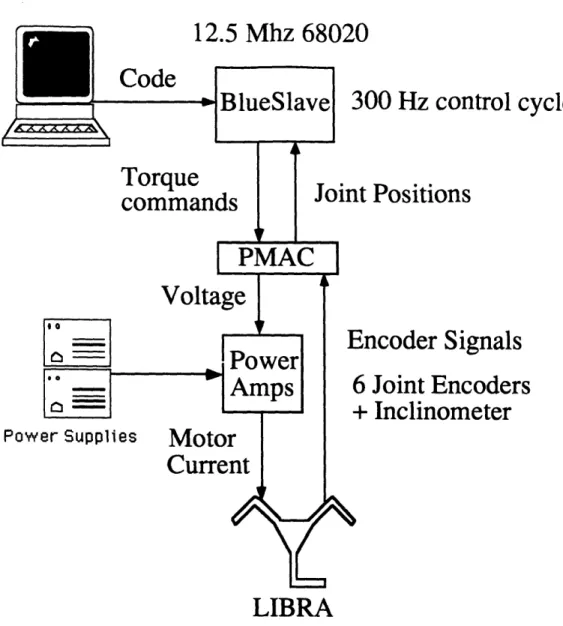
A block diagram of the experimental setup is shown in Figure 14. It consists of the mechanical LIBRA climbing machine, the power amplifiers, and the control computers. Each part of the system is described in the following sections.

Code

LIBRA

Fig. 14: LIBRA system block diagram

4.1.1: Climbing Machine

The mechanical configuration of the LIBRA is shown in Figure 15. It consists of a main body with three limbs (legs), each with two links and two actuated joints. The angles 01 through 06 are the joint angles of the actuated joints. The angles 02 and 03 are measured with respect to the line passing through joint 2 and joint 3. The angle 05 is measured with respect to the normal of this line passing through joint five. All angles are measured in a counterclockwise direction. The angle 0 is a reference angle between the inertial coordinate frame and limb 1. The angle 0 is not measured directly, but is calculated using the constraint equation for the y location of limb 2.

I

00 Hz control cycle

Positions

ncoder Signals

Joint Encoders

Inclinometer

/7

Limb 2

04

'X

Body

INERTIAL

COORDINATE

FRAMIE

Limb 3

06

Fig. 15: A Schematic of the LIBRA

The joint vector, consisting of the angles 0 of the actuated joints, is defined as:

q

=

101,02,03=45,e,06

T

The actuated joints are driven by Escap 23DT12 -216E electric motors with a 792:1 gear ratio transmission. The large gear ratio was required to produce relatively large torques using small motors. The large gear ratio has several drawbacks, including large transmission friction, poor back-drivability, and significant backlash in the output shaft of two degrees. The motor and gearhead specifications are 54:

Torque Constant = 23.3 mNm/A

Back EMF Constant = 0.0024 V/rpm

No-Load Current = 20 mA

Maximum Continuous Current = 0.9 A Armature Resistance (Rm) = 9.7 Ui Armature Inductance (Lm) = 0.8 mH

Maximum Dynamic Torque = 4.5 Nm @ 20 rpm Maximum Static Torque = 20 Nm @ 0 rpm Gearhead Efficiency (11) = 0.55

Max. input speed = 3000 rpm

The ranges of the joint angles are limited by the mounting hardware off the actuators. The joint limits are given as:

Joint 1 = ± 117" Joint 2 = + 132", -69" Joint 3 = + 1320, -69" Joint 4 = ± 1170 Joint 5 = ± 110" Joint 6 = ± 117"

The on-board sensors consist of encoders measuring the joint angles and a pendulum-based inclinometer used to measure the angle of the center body (OB). The inclinometer is necessary to obtain the initial orientation, and it is also used to confirm the position of the system as it climbs. The encoders on the motor have a resolution of 2000 counts per revolution of the motor shaft, after utilizing quadrature decoding to enhance the resolution. The gearhead increases this to 1,584,000 counts per revolution of the output shaft. However, the accuracy of the encoder is still limited by the backlash in the output shaft. The inclinometer has a resolution of 0.35 degrees, but stiction limits its sensing accuracy to ± 1 degree. A force sensor was mounted on a ladder step to measure the horizontal force applied by foot 2, but the sensor was only used for collecting data and did not provide feedback to the control loop.

The LIBRA has a limb span of 0.7 meters, and weighs 8 kg. Rubber model airplane wheels 8.3 cm in diameter are used as the end-effectors. Several advantages to using the compliant wheels are: limited impact force, good contact stability, easy seating of the wheels in the steps, and simplicity of building. Hooks are being considered to allow climbing on one ladder and a variety of other climbing gaits. Details of the construction of the LIBRA can be found in 1. Modifications performed on the LIBRA not documented in Argaez 1 are minor: some material was removed from the components to reduce weight, and the motor shaft clamps were rebuilt using a friction clamp design, rather than a set screw.

The ladders that are climbed by the LIBRA are constructed of angle iron, providing adjustable step height and L shaped steps. The configuration used for the LIBRA experiments discussed in this thesis are a ladder separation of 0.18 m, and a uniform step height of 0.134 m.

4.1.2: Power Amplifiers

The power amplifiers are voltage to current amplifiers, acting as variable current sources. Their schematics and other details can be found in Appendix B. The amplifier-motor system has a time constant of 1.52 microseconds, resulting in a bandwidth of 656 Hz. Since this far exceeds the bandwidth of the controller, we can treat the amplifier-motor systems as torque servos. However, this does not include the damping resulting from the large friction found in the gearheads. This will result in additional damping

added to the system.

4.1.3: Control Computers

A VME bus computer system running VxWorks is used to control the LIBRA. A Sun 3/80 workstation is used to program, debug, and compile the control code, and for data storage. The compiled control software is then downloaded to run on a 68020, 12.5 MHz processor. The control cycle closes at a rate of 300 Hz. A multi-axis control board mounted on the VME bus, called the Erogrammable Multi Axis Controller (PMAC) 55, is used to decode and count the encoder signals and as D/A converters to output the control signals. The PMAC was able to perform these tasks at a rate of 1000 Hz.

Work is currently being done to implement the control software on a custom-made computer board designed to mount on the LIBRA itself. The board consists of 6 motor control chips and one 8031 processor. This board is representative of the computing capability available for many small robots.

4.2: Climbing Gait

The LIBRA is designed to climb between two ladders. Currently only one climbing gait is used. It is a four stage gait, shown in Figure 16. Stage one starts with a pushup maneuver to get its body level with the next set of rungs, and then places its third foot on the right hand ladder. In stage two, the LIBRA lifts the second foot off of the rung and lets foot 3 support the body. Foot 2 then lifts up one rung, and transfers back to the support of the body at the start of stage three. Foot 3 then swings over to the left hand rung. In stage four, foot 1 lifts up one rung. The cycle then repeats itself, continuing the climb.

Stage 1 : Foot 3 swings to right step Stage 2 : Foot 2 lifts one step

Stage 3 : Foot 3 swings to left step Stage 4 : Foot 1 lifts one step

4.3: Control Vector Selection

As can be seen from the above description of the climbing gait, in stages one and three it is desirable for the task of climbing to control the x, y, and theta positions of the center body and the x and y positions of foot 3. A detailed Extended Mobility Analysis is performed to test if this is an acceptable set of control variables. A Gruebler's mobility analysis performed on the LIBRA system with pin joints at two of the feet as shown in Figure 17 reveals that the system has five DOF (F=a=b=5).

1=8

fl=8

f2=0

F=a=5 b=5

Fig. 17: LIBRA under full environmental constraints

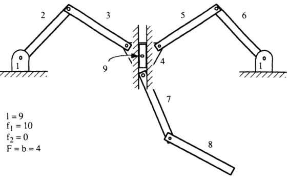
Constraining the x position (placing a vertical slider on the center body as shown in Figure 18) and performing another mobility analysis gives only four DOF (b=4), so the x position of the center body is an acceptable control variable.

1=9 f, = 10

f2 = 0 F=b=4

Fig. 18: Constraining x of the Center Body

Adding a constraint on the y position of the center body also results in the loss of a degree of freedom, as shown in Figure 19 (b=3).

1=8 fl =9 f2= 0

F=b=3

Fig. 19: Constraining x,y of the Center Body

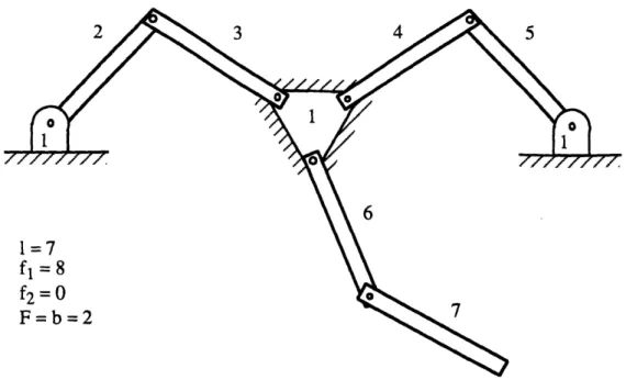
Immobilizing the center body by adding a 0 constraint also reduces the degrees of freedom (b=2).

1=7 fl= 8

f2=0

F=b=2

Fig. 20: Constraining x,y,0 of the Center Body

It is obvious that constraining the x and y of the free foot will completely constrain the system, as shown in Figure 21.

1=7 fl=9

f2=0

F=b=O