HAL Id: hal-00302068
https://hal.archives-ouvertes.fr/hal-00302068
Submitted on 1 Jan 2002
HAL is a multi-disciplinary open access
archive for the deposit and dissemination of
sci-entific research documents, whether they are
pub-lished or not. The documents may come from
teaching and research institutions in France or
abroad, or from public or private research centers.
L’archive ouverte pluridisciplinaire HAL, est
destinée au dépôt et à la diffusion de documents
scientifiques de niveau recherche, publiés ou non,
émanant des établissements d’enseignement et de
recherche français ou étrangers, des laboratoires
publics ou privés.
Self-sustained oscillator as a model for explosion quakes
at Stromboli Volcano
S. de Martino, C. Godano, M. Falanga
To cite this version:
S. de Martino, C. Godano, M. Falanga. Self-sustained oscillator as a model for explosion quakes at
Stromboli Volcano. Nonlinear Processes in Geophysics, European Geosciences Union (EGU), 2002, 9
(1), pp.31-35. �hal-00302068�
Nonlinear Processes
in Geophysics
c
European Geophysical Society 2002
Self-sustained oscillator as a model for explosion quakes at
Stromboli Volcano
S. De Martino1,3, C. Godano2, and M. Falanga1,3
1Department of Physics, Salerno University, Via S. Allende, Baronissi (SA) 84084 Italy
2Dipartimento di Scienze Ambientali, II Universita’ di Napoli, Caserta, Italy
3INFM unita’ di Salerno, 84081 Baronissi (SA), Italy
Received: 8 March 2001 – Revised: 1 June 2001 – Accepted: 25 June 2001
Abstract. We analyze seismic signals produced by explosion-quakes at Stromboli Volcano. We use standard nonlinear procedures to search a low-order effective dynam-ics. The dimension of the reconstructed phase space depends on the number of samples. Namely larger time lengths cor-respond to dynamical systems of different complexity. If we restrict the analysis to the signal associated directly to the source (Chouet et al., 1997), we obtain a phase space dimen-sion equal to two. We reproduce this part of the signal with a simple single self-sustained oscillator.
1 Introduction
In basaltic eruptions, the relative motion of the gas with re-spect to the liquid produces either an anular flow (Hawa-ian Fire Fountains) or a Slug flow (Strombol(Hawa-ian explosions). Both behaviours are generated by complex processes of magma flow and turbulent degassing. The dynamics underly-ing the generation of these behaviours is not well understood, even though experiments on laboratory scale (Jaupaurt et al., 1988; Mader et al., 1994) have reproduced well some of their characteristics.
Theoretical models have been produced and much insight on the processes has come from acoustic emission studies (Ripepe et al., 1999; Schik et al., 1988; Vergniolle et al., 1996) . In this paper we focus on the Strombolian explo-sion quakes to reconstruct a dynamical system that can rep-resent the source in this regime. We assume a complemen-tary point of view, compared with the many fruitful models previously quoted that look at the generation of a slug from the degassing process and that want to reproduce the var-ious features of acoustic emission and seismic signals. In fact, following the line of the seminal paper of Chouet and Shaw (Chouet et al., 1991) we want to extract from the ex-plosion quakes signals recorded at Stromboli some “essential dynamics”. In other words, we seek a dynamical model that
Correspondence to: S. De Martino ([email protected])
can represent either the average properties or some of the universal features of the complex dynamics generating these seismic signals. We use standard methods (see, for example Abarbanel, 1995, and references therein) to extract essential dynamics from the the experimental time series. As we shall see the phase space dimension of the “effective dynamical system”, in our case, depend on the time length of the sam-ple. This is due to the fact that by increasing the sample length we look at the same dynamical system, with a more and more complex structure. We find that the correlation di-mension of the attractor (which gives the number of variables
involved in the effective dynamics) is in the range da=2÷3.
Then there are low-dimension dynamics that can be consid-ered as an effective description of a complex physical system that generates the signal. Starting from this result, we try to simulate the first few seconds with a simple self-sustained oscillator. It is actually in this part that conventional wisdom recognizes a well distinguished trace of the source. We ob-tain the true signal from the analytical model in the regime of a limit cycle.
2 Data
We select explosion-quakes to study seismic signals recorded in April 1992 with small arrays of seismometers, by USGS, University of Aquila and Vesuvian Observatory. An accu-rate description of the deployed network and the instrumen-tation can be found in Chouet et al. (1997). We are specif-ically interested in the following: the wavefield effectively comes from craters and it is composed of body waves in the first few seconds (see also Del Pezzo et al., 1992). In or-der to extrapolate an “effective” dynamics from the scalar time series, we apply some standard techniques of smooth-ing. The aim of these procedures (described in the follow-ing) is to eliminate the high dimensionality due to the scat-tering with respect to the dimensions of the source dynamics; note that these operations do not affect the spectral content of the signal. First, we introduce the usual instrumental
correc-32 S. De Martino et al.: Self-sustained model for Stromboli explosion quakes 0 2 4 6 8 10 12 14 16 18 20 −2 −1.5 −1 −0.5 0 0.5 1 1.5 2 Time (s) Amplitude
Fig. 1. Normalized amplitude of the average earthquake after the
application of the nonlinear denoising.
tion. Then we construct an average earthquake using beam forming based on the knowledge of the apparent velocity of the first pulse and of the position of the stations. This av-erage signal was built using 70 explosion-quakes recorded at 15 stations. This filters the background scattering radi-ation generated by the random distribution of the points of scattering. Then we correct the signal for the envelope in or-der to make it stationary at the second oror-der, i.e. we impose that the signal has to mean of zero and constant variance. This is necessary since superimposed dissipative dynamics causes the phase space to contract at a point, preventing the presence of an attractor representative of effective dynamics. Finally, we eliminate the noise by means of a nonlinear tech-nique. We prefer to use this method rather than the standard linear filter. Namely the signals from nonlinear sources can exhibit genuine broad band spectrum and there is no justifi-cation to identify any part of spectrum as noise as necessary using spectral or other linear filters. The nonlinear denois-ing takes into account the fact that deterministic signals form smeared-out lower dimensional manifolds, then the denois-ing identifies such a structure and projects the signal onto these manifolds in order to reduce the noise (see Grassberger et al., 1993; Kostelich et al., 1993). The final signal is shown in Fig. 1. Again, these transformations do not affect the spec-tral content of the signal. Now we are ready to perform our analysis.
3 Phase space reconstruction
As stated in the introduction, we wish to recognize the low dimension dynamics of the seismic signal recorded at Strom-boli Volcano by reconstructing the phase space.
It is well-known that any dynamic process is characterized by the trajectories in the phase space. In some cases they are confined to a limited portion of the whole space defin-ing an attractor of the dynamics. Sometimes the dimension
of the attractor is fractal, thus the attractor is called strange. A standard procedure in the analysis of experimental data to reconstruct the asymptotic time evolution is to use the time delay method. This method relays on the mathematical for-mulation due to Takens (1981). If
n si
on
i=1 (1)
is a time series of n scalar observations sampled at equal in-tervals (our explosion-quake signal), the reconstructed attrac-tor consists of points of the form
xi =(si, si+τ, ..., si+(m−1)∗τ), (2)
where m is the embedding dimension and τ is the time de-lay. Takens shows, under suitable hypotheses, that this re-construction is equivalent to the original attractor if m is large enough. Thus the numerical problem is to determine m and
τ. There is a lot of literature on this problem (see, for
exam-ple, Abarbanel, 1995). Among different but in essence equiv-alent methods we select mutual information (Fraser et al., 1986) and false nearest neighbours (Kennel et al., 1992) to calculate, respectively, the time delay and embedding di-mension. Mutual information is the extension of the auto-correlation function to the nonlinear domain. The false near-est neighbours technique is based on the projection of the points of the dynamics onto spaces of increasing embedding dimensions. The points appear nearest to the neighbours of some others until the dimension becomes the proper one of our embedding space. When the fraction of these false near-est neighbours with respect to the total number of points is zero, then we can stop our process. Note that the value of m, so obtained, does not represent the value of the embedding
dimension used to estimate the dimension of the attractor da;
indeed it represents the lower limit for the embedding
dimen-sion necessary to evaluate da. Moreover, it is an upper bound
for da. Now we are able to estimate the dimension of the
attractor. In order to do this, we use the standard technique of Grassberger et al. (1983) based on the calculation of the correlation integral C(l) = 1 N X i 1 N −1 X j 6=i ϑ (l− |xi−xj |), (3)
where xiare the vectors previously defined in Eq. (2), and ϑ
is the Heaviside function. The slope of C(l) in the scaling region (where it has a power law behaviour) is the
correla-tion dimension of the attractor. Here we evaluate da first in
a moving window of 3.5 s. This choice of window length is due to our capability to model only about 3.5 s of the signal:
we have to compare daof experimental data with daof
simu-lated signal. C(l) can be evaluated for different values of the
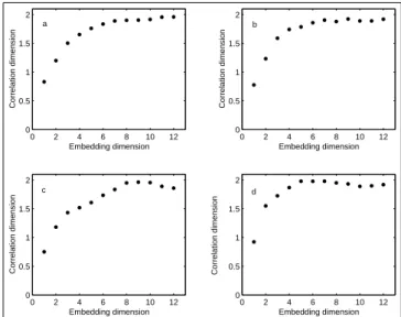
embedding dimension, up to a value at which dasaturates. In
Figs. 2a–2d we show da versus m for the value of τ (0.07 s
for all windows) selected with mutual information. Then we perform the same analysis on the other two windows (10 and
20 s). Although the estimated da for the last two windows
Table 1. The correlation dimensions dafor the adjacent time win-dows of 3.5 s; m is the embedding dimension as evaluated by means of false nearest neighbours
Time windows (3.5 s) da m
first window 1.92 2 second window 1.90 2 third window 1.93 3 forth window 1.94 3
Table 2. The correlation dimensions dafor the time windows,
re-spectively, of 10 s and 20 s. Again m is the embedding dimension as evaluated by means of false nearest neighbours
Time windows (s) da m
10 2.4 3 20 2.8 5
of the evaluation for da, these values contain some
informa-tion on the evoluinforma-tion of dynamics and on the stainforma-tionarity of our signal. The choice of the window length is also deter-mined from the results of Chouet et al. (1997) who suggest that the source is limited to the first 10 s of the signal while the other part is affected by strong scattering. The analogue of Fig. 2 for the other two windows is shown in Fig. 3. The dimensions of the various attractors, reproducing the effec-tive dynamics for the three different window lengths, change from about two up to about three (see Tables 1 and 2).
These results are in good agreement with the previous ones: Capuano et al. (1999) obtained a fractal dimension
da =2.75 for the whole signal. It’s very interesting to note
that the bidimensional projections of the reconstructed phase space (in the first few seconds this is the proper phase space
because da'2) exhibit a behaviour close to a limit cycle, as
one can see in Fig. 4a.
Figures 4b–d show the reconstructed phase space for the other three adjacent 3.5 s time windows. As we can see in particular in the last two, even if the dimension is lower than two, the scattering becomes present, partly obscuring the presence of a limit cycle. Finally, Fig. 4e and f show the phase space for time windows of 10 and 20 s.
4 Analytical effective dynamical model for the source
The result of a dimension equal to two for the first few sec-onds of the signal could lead us to interpret our observation in terms of an harmonic oscillator, but the variability of the di-mension throughout the time indicates the presence of a more complex dynamics (with a strange attractor and a dimension
2 < da <3) which starts its evolution over a limit cycle. A
complete model of our signal requires a fluid-dynamic
equa-0 2 4 6 8 10 12 0 0.5 1 1.5 2 Embedding dimension Correlation dimension 0 2 4 6 8 10 12 0 0.5 1 1.5 2 Embedding dimension Correlation dimension 0 2 4 6 8 10 12 0 0.5 1 1.5 2 Embedding dimension Correlation dimension 0 2 4 6 8 10 12 0 0.5 1 1.5 2 Embedding dimension Correlation dimension a b c d
Fig. 2. Correlation dimension vs. embedding dimension as
esti-mated by means of Grassberger and Procaccia method for the fourth adjacent 3.5 s time windows. As we can see, in all cases, datends
toward two.
tion reproducing the signal and the phase space of Strom-bolian earthquakes. Here we limit our attention on an ana-logic model which should reproduce the characteristics of our signals. The idea is to choose, among various nonlin-ear oscillators, the one that best fits our data. The choice of a self-sustained oscillator has no particular reason except the one that it is the simplest nonlinear oscillator for which nonlinearity is clearly recognizable in the balancing of dis-sipation and loading mechanisms. An analogical example of self-sustained oscillations can be furnished by a valve os-cillator with the oscillating circuit in the anode circuit and inductive feedback. Nonlinearity is produced by the mutual dependence between grid voltage and anodic current by in-ductive feedback. The system is described by the following adimensional couple of equations:
¨
x + h1x + h˙ 3x =0 for x < b,
¨
x − h2x + h˙ 3x =0 for x > b. (4)
where b is the first point of return of the limit cycle; x is referred to a variable dynamically significant (current in the case of valve oscillator, ground displacement in our case);
h3is a parameter connected to the characteristic frequency;
h1is a dissipation parameter and h2is a loading parameter.
For a detailed description of this equation, see Andronov et
al. (1937). A discussion of the true physical meaning of h1,
h2, h3is not possible at this stage, because our modelling is
only analogic (see conclusion).
We fix b observing the first return of the trajectory in the
reconstructed phase space. To estimate the parameters h1,
h2and h3, we construct a tridimensional matrix, whose
ele-ments generate, separately, a signal that can be compared to the true signal. We choose the best term in a sense of mini-mum square, i.e. we fix those parameters that generate a min-imum root mean square deviation with respect to the original
34 S. De Martino et al.: Self-sustained model for Stromboli explosion quakes 0 2 4 6 8 10 12 0 0.5 1 1.5 2 2.5 Embedding dimension Correlation dimension 0 2 4 6 8 10 12 14 0 0.5 1 1.5 2 2.5 3 Embedding dimension Correlation dimension a b
Fig. 3. Correlation dimension vs. embedding dimension as
esti-mated by means of Grassberger and Procaccia method for two win-dows, respectively (a) 10 s and (b) 20 s long.
signal. The value of ω so obtained corresponds, within the statistical errors, to the first peak of the FFT of the original average earthquake, i.e. 1.1 Hz. In Fig. 5 one can observe the original signal and the simulated one. The correlation coeffi-cient between the two signals is r = 0.98, the corresponding standard deviation is 0.04. By changing instantaneously the value of b, it is possible to also simulate the next part of the signal, composed of the other 3–4 s. The entire signal can be obtained using Eq. (4) and introducing, where necessary, a short time instability by hand.
We have considered the explosion-quakes seismic signals of the Stromboli Volcano by studying their behaviour by means of standard non linear analysis of dynamical systems. The aim was to reconstruct an effective low-dimension dy-namics characterizing the Stromboli source during this tran-sient regime.
5 Conclusions
As a result, we have extracted phase space dimensions for the asymptotic time evolution. The dimension depends on the time length of the sample considered and ranges from 2 to 2.80. This result could suggest that the signal is not sta-tionary, but very simple statistical tests (multivariate analysis of the average value and of the variance) reveal that it is sta-tionary at the first and second order. Such a peculiar result cannot be easily explained, but we suggest that the dynamics evolves in such a way that the whole phase space, in the first seconds, is not visible. In other words, the system should be in a stationary state which can be viewed only looking at the whole signal. The first seconds of the signals evolve on a stationary state but on a manifold of the phase space of lower dimensionality. −2 −1 0 1 2 −2 −1 0 1 2 x(t) x(t+0.07) −2 −1 0 1 2 −2 −1 0 1 2 x(t) x(t+0.07) −2 −1 0 1 2 −2 −1 0 1 2 x(t) x(t+0.07) −2 −1 0 1 2 −2 −1 0 1 2 x(t) x(t+0.07) −2 −1 0 1 2 −2 −1 0 1 2 x(t) x(t+0.07) −2 −1 0 1 2 −2 −1 0 1 2 x(t) x(t+0.07) a b c d e f
Fig. 4. Bidimensional projections of the reconstructed phase space
with τ = 0.07 s. Figures (a), (b), (c), (d) show the phase space relative to 3.5 s time windows. Figure (e) shows the phase space of 10 s and Fig. (f) shows one relatively to the whole earthquake.
0 50 100 150 200 250 300 350 400 450 −0.25 −0.2 −0.15 −0.1 −0.05 0 0.05 0.1 0.15 0.2 0.25 samples simulated quake original quake RMS=0.02r=0.98
Fig. 5. Simulated earthquake and original one for the first 3.5 s
(directly connected to the source); the coefficient of correlation is
r =0.98 and RMS=0.02.
We have focused our attention on this manifold because it is very simple to be reproduced. We have simulated these first seconds of the signal taking the general Eq. (4). This
equation can give, fixing suitable parameters h1, h2, h3and
b, all kinds of behaviour, i.e. harmonic, forced, damped and
self-sustained oscillations. The best fit with the correlation equal to 0.98 and RMS equal to 0.04 singled out the self-sustained oscillator in the limit-cycle regime (see Fig. 5).
The estimated values of h1 and h2 give a numerical
ac-count of the balancing between dissipation and loading en-ergy onto the magmatic system to generate the seismic sig-nal. The characteristic oscillation frequency of this
sig-nal. Note that our simulation is based on an analogic model which is able to simply reproduce the signal; this implies that a physical model should be based on more general equa-tions which, with some simplification or averaging, should be transformed into Eq. (4). This and the reproduction of the whole phase space should be a matter of forthcoming papers.
References
Abarbanel, H. D. I.: Analysis of Observed Chaotic Data, Springer-Verlag, New York, Berlin, 1995.
Andronov, A. A., Vitt, A. A., and Khaikin, S. E.: Theory of oscilla-tors, 1937, Republished Dover Publications, Inc., 1966. Capuano, P. and Godano, C.: Source characterisation of low
fre-quency events at Stromboli and Vulcano Islands (isole Eolie Italy), J. Seism, 3, 393–408, 1999.
Chouet, B. A. and Shaw, H. R.: Fractal properties of tremor and gas-piston events at Kilauea Volcano, Hawaii, J. Geophys. Res., 96, 1991.
Chouet, B. A., Saccorotti, G., Martini, M., Dawson, P., De Luca, G., Milana, G., and Scarpa, R.: Source and path effect in wavefield of tremor and explosions at Stromboli Volcano, Italy, J. Geophys. Res., 102, 15 129–15 150, 1997.
Del Pezzo, E., Godano, C., Gorini, A., and Martini, M.: Wave po-larization and location of the source of the explosion quakes at Stromboli Volcano, IAVCEI Proceedings, in: Volcanology, (Eds) Gasparini, P., Scarpa, R., and Aki, K., Springer-Verlag, Berlin, 3, 279–295, 1992.
Fraser, A. M. and Swinney, H. L.: Independent coordinates for strange attractors from mutual information, Phys. Rev. A, 33,
1134–1139, 1986.
Grassberger, P. and Procaccia, I.: Measuring the strangeness of strange attractors, Physica D, 9, 189–208, 1983.
Grassberger, P., Hegger, R., Kanz, H., Schaffrath, C., and Schreiber, T.: On noise reduction methods for chaotic data, CHAOS, 3, 127, 1993.
Jaupart, C. and Vergniolle, S.: Laboratory models of Hawaiian and Strombolian eruptions, Nature, 331, 58–60, 1988.
Kennel, M. B., Brown, R., and Abarbanel, H. D. I.: Determining embedding dimension for phase space-reconstruction using a ge-ometrical construction, Phys. Rev. A, 45, 3403–3411, 1992. Kostelich, E. J. and Schreiber, T.: Noise reduction in chaotic time
series data: A survey of common methods, Phys. Rev. E, 48, 1752–1763, 1993.
Mader, H. M., Zhang, Y., Phillips, J. C., Sparks, R. S., Sturtemant, B., and Stolper, E.: Experimental simulations of explosive de-gassing of magma, Nature, 372, 85–88, 1994.
Ripepe, M. and Gordeev, E.: Gas bubble dynamics model for shal-low volcanic tremor at Stromboli, J. Geophys. Res., 104, 10 639– 10 654, 1999.
Schick, R. and Mueller, W.: Volcanic activity and eruption se-quences at Stromboli during 1983–1984, Modelling of Volcanic Processes, (Eds) Chi-Yu King and Scarpa, Fr. Vieweg & Son, Wiesbaden, 120–139, 1988.
Takens, F.: Detecting Strange Attractors in Turbolence, in Dynam-ical Systems and Turbolence Warwick, 1980, in Lectures Notes in Mathematics, 898, 366–381, Springer Berlin, 1981.
Vergniolle, S. and Brandeis, G.: Strombolian explosions 1. A large bubble breaking at the surface of a lava column as a source of sound, J. Geophys. Res., 101, 20 433–20 447, 1996.