Seasonal dynamics of phytoplankton and Calanus finmarchicus in the North Sea as revealed by a coupled one-dimensional model

(1)

HAL Id: hal-02987472

https://hal.archives-ouvertes.fr/hal-02987472

Submitted on 6 May 2021

HAL is a multi-disciplinary open access

archive for the deposit and dissemination of sci-entific research documents, whether they are pub-lished or not. The documents may come from teaching and research institutions in France or abroad, or from public or private research centers.

L’archive ouverte pluridisciplinaire HAL, est destinée au dépôt et à la diffusion de documents scientifiques de niveau recherche, publiés ou non, émanant des établissements d’enseignement et de recherche français ou étrangers, des laboratoires publics ou privés.

Distributed under a Creative Commons Attribution| 4.0 International License

Seasonal dynamics of phytoplankton and Calanus

finmarchicus in the North Sea as revealed by a coupled

one-dimensional model

Francois Carlotti, Günther Radach

To cite this version:

Francois Carlotti, Günther Radach. Seasonal dynamics of phytoplankton and Calanus finmarchi-cus in the North Sea as revealed by a coupled one-dimensional model. Limnology and Oceanog-raphy Bulletin, American Society of Limnology and OceanogOceanog-raphy, 1996, 41 (3), pp.522-539. �10.4319/lo.1996.41.3.0522�. �hal-02987472�

(2)

Limnol. Oceanogr., 4 l(3), 1996,522-539

0 1996, by the American Society of Limnology and Oceanography, Inc.

Seasonal dynamics of phytoplankton and Calanus jnm:archicus in the

North Sea as revealed by a coupled one-dimensional model

Franqois Carlotti

Station Zoologique, URA CNRS 7 16, BP 28, F-06230 Villefranche-sur-Mer, France

Giinther Radach

Institut fiir Meereskunde, Troplowitzstr. 7, 22529 Hamburg, Germany

Abstract

A population dynamics model for Calanusjbnarchicus was coupled with a one-dimensional physical and biological upper layer model for phosphate and phytoplankton to simulate the development of the successive stages of Calanus and study the role of these stages in the dynamics of the northern North Sea ecosystem. The copepod model links trophic processes and population dynamics, and simulates individual growth within stages and the changes in biomass between stages.

Simulations of annual cycles contain two or three generations of Calanus and indicate the importance of growth of late stages to total population biomass. The spring peak of zooplankton lags that of phytoplankton by a month due to growth of the first cohort. When compared with observations, the simulation shows a broad phytoplankton bloom and a low biomass of Calanus. A higher initial overwintering stock changes the dynamics of Calanus, but not the annual biomass. The timing of the spring ascent of overwintering individuals influences subsequent dynamics.

Simulations of spring dynamics compared with data obtained during the Fladen Ground Experiment in 1976 show that grazing by Calanus cannot be the only major cause limiting the phytoplankton bloom because development of the first stages of Calanus is slow, and the last copepodite stages arrive after the bloom. Calanus never attains realistic biomasses feeding on phytoplankton as a single food source. These simulations led us to add a compartment of pelagic detritus, which provides another food source to enable Calanus population growth.

The interactions between physical and biological processes are an important part of planktonic ecosystem dynamics; however, studying these processes simultaneously often is difficult because of different time and space scales (Mar. Zooplankton Colloq. 1 1989). During the last

decade, several workers (e.g. Mullin et al. 1985; Wro- blewski and Richmann 1987; Kicdrboe and Nielsen 1990) have demonstrated the important role of physical mixing on temporal scales of from a few days to several years for primary and secondary production. Primary production depends mainly on the stability of the water column; strong vertical mixing initially reduces production but supplies the upper water column with nutrients and there- by stimulates subsequent production. Not only is copepod production considered dependent on phytoplankton production, but these dynamics over small time and space scales may also attenuate trophic variability, ultimately

Acknowledgments

This work was completed while F.C. was a postdoctoral fellow at the Institut ftir Meereskunde der Universiti-3 Hamburg and was supported by a research stipend of Alexander von Hum- boldt Stiftung and by a fellowship from the STEP program of EEC. CNRS/INSU and URA 7 16 allowed F.C. to work in Ham- burg in 1992.

We thank Andreas Moll for advice and Ortrud Kleinow and Matthias Regener for computer programming assistance. We also thank the anonymous reviewers and B. P. Boudreau and J. Dolan for comments and suggestions that helped to clarify the manuscript.

affecting the reLationship between primary production and fisheries (Runge 1988). Events such as storms or intense heating may have severe consequences for the structure of the whole food chain, including fish recruitment (Mul- lin et al. 198511.

Our understanding of the role that time-limited events play in long-range ecosystem dynamics is largely based on dynamics simulations with mixed-layer models that couple nutrient and plankton dynamics (see Fransz et al. 199 1 b). However, most of these models take into account only nutrients and phytoplankton (Fransz et al. 199 1 b), probably beta Jse of the difficulty of representing the complex behavior that exists among zooplankton species and also among the different zooplankton developmental stages. Models having one compartment for the whole zooplankton community are useful only for simulating ecosystem dynamics over the course of a few days (Wro- blewski and Richman 1987) or for a stable environment but become meaningless for long periods if the environment fluctuates. Although field workers consider population dynamics to be the minimum level of study, zooplankton population models are rarely included in ecosystem models. Steele and Henderson (1976) demonstrated that a comprehensive model of the North Sea food chain needs to take into account the population dynamics of CalanusJi~zmarchicus. Our goal is to define how and when such coupling of phytoplankton and zooplankton is truly necessary. As an example, we use C. finmarchicus in the North Sea; this species dominates the biomass of zooplankton in spring and summer and shows clearly

(3)

Production in the North Sea 523

[m +

f I

Sedimentation

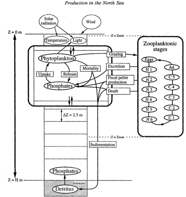
Fig. 1. Conceptual diagram of the coupled model. A stage dynamics model for CaZanus jnmarchicus, evenly distributed within a given layer, has been coupled with a 1-D vertically

resolved physical and biological model. The physical submodel drives the dynamics of nutrients, phytoplankton, and benthic detritus. Formulations of processes are detailed by Radach and Moll (1993). Processes coupling the population of copepods to the ecosystem are given in Table 2.

demarcated cohorts. In fall, other species, such as Cen- tropages typicus, take its place (Fransz et al. 199 la).

Recently, Radach and Moll (1993) developed a one- dimensional (1 -D) physical and biological upper-layer model. This model simulates the annual cycles of the physical dynamics in the water column and the biological dynamics of phytoplankton and phosphate and estimates annual primary production in the central North Sea. Ra- dach and Moll correlated these results with meteorological observations and estimated radiation data spanning 25 yr and clearly demonstrated the role played by short- term events in integrated annual production. In Radach and Moll’s model, zooplankton were a forcing variable. In our paper, we combined their model with a population dynamics model for C. Jinmarchicus, similar to that de-

scribed by Carlotti and Nival (1992). These two models have been independently calibrated and validated.

The model

Concept of the coupled model-We searched for the simplest model to explain the main features of plankton dynamics, including the dynamics of C. Jinmarchicus in the central and northern North Sea. Because the system is nonlinear, we deliberately did not choose the most complete but most complex model. Instead, we kept the structure of both simple submodels (Fig. 1) and added a “compartment” for pelagic detritus, which was not previously represented.

(4)

524 Carlotti and Radach

Radach and Moll’s (1993) model consists of three submodels: a meteorological submodel that drives both a 1 -D vertical submodel for the physics of the upper layer and a biological submodel, which also is driven by output from the physical model. We do not discuss the meteorological and physical submodels (see Radach and Moll

1993), but focus on the biological submodel. This submodel describes nutrient and phytoplankton dynamics in the water column and benthic deposition of detritus. Phy- toplankton development depends on the supply of light and nutrients. Self-shading is also represented in the model. Phytoplankton produce new biomass, release catabolic substances, are affected by turbulent diffusion and sinking, and are either grazed on by zooplankton or deposited on the seabed. In the phytoplankton submodel, organic detritus in the water column is either immediately remineralized or directly transported to the bottom, where it accumulates in a stock of benthic detritus. The pool of nutrients is enriched in many ways: through benthic re- generation and turbulent diffusion; remineralization of dead phytoplankton, dead copepods, and fecal pellets; release from phytoplankton cells; and zooplankton excretion. The benthic detritus pool receives a flux of dead phytoplankton, fecal pellets, and dead zooplankton from the entire water column. Part of this detritus is remineralized in the water column, producing regenerated nutrients. The equations for the model are given by Radach and Moll (1993).

The copepod submodel can be divided into two levels: the first corresponds to the developmental instars (eggs, nauplii, copepodites, and adults), and the second is con- cerned with the age classes in each stage. In each age class, the variations of mean individual weight and the numbers of individuals are calculated as a function of various linked biological processes according to the conceptual model presented by Carlotti and Sciandra (1989, their figure 1). The growth rate and weight govern the processes of natural mortality, molting, and egg production. The model was conceived originally for Euterpina acutifrons, a small copepod without reserves. In our model of C. jinmarchicus, we did not represent the accumulation of reserves because the North Sea population has a low fat content (except for overwintering individuals) compared to populations that stay in the North Atlantic (Carlotti et al. 1993).

Adaptation of the submodel to Calanus finmarchicus- Previously, we showed (Carlotti and Sciandra 1989; Car- lotti and Nival 1992) that the zooplankton submodel can represent some fundamental functional relationships between the level of individuals and the level of the population. The mathematical formulations of the processes were presented by Carlotti and Sciandra (1989, their table

1).

The only changes we made to Carlotti and Sciandra’s model was to the function fl -the dependence of the ingestion rate on the food concentration- and we adopted the double rectilinear model of Gamble (1978) rather than use the Ivlev-Parsons relationship (Carlotti and Sciandra 1989). The parameters of this function are the maximal

ingestion rate (Pl), the minimal threshold food concentration (P2), and the optimal food concentration (P3) that maximizes grazng rate. The values for all parameters are given in Table 1. The ingestion rate depends on the developmental stage, food supply, temperature, and weight of the animals. The first two naupliar stages of C. Jin- marchicus are unable to ingest particles; they are considered to live on reserves provided by the egg (Corner et al. 1967). For the other naupliar stages, we have the results of Fernandez ( 1979, his figure 3), who obtained maximum grazing rates of 0.4, 0.6, 1 .O, and 1.5 pg C ind-l d- I, respective1 y, for N3-N6 of C. pacijkus at 15°C. Nau- pliar grazing rates at 8°C were deduced from a function of temperature and are explained below. Daro (1980) estimated the maximal ingestion rates at 8°C during the Fladen Ground Experiment in 1976 (FLEX’76) to be 1, 5, 10, 15, and 20 pg C ind-l d-l, respectively, for Cl- C5; Gamble (1978) estimated 25 pg C female-l d-l. The values of Pl are deduced by dividing these values by the body weight at. 8°C. The threshold food concentration (P2) is equal to 50 pg C liter-l for copepodite and adult stages (Daro 1980; Gamble 1978), but we chose a lower threshold of 20 pg C liter- l for nauplii (Mullin and Brooks 1976; Fernandez 1979). The optimal food concentration (P3) for which ingestion is maximal also increases with each stage (Mullin and Brooks 1976). During FLEX’76, Gamble (1978) and Daro (1980) obtained a value of 150 pg C liter- l for copepodites and adults. We fixed the value of P3 for the nauplii at 100 pg C liter-l.

We use a value of 2.1 for QlO, which is the value estimated by Gamble (1978) for C. jnmarchicus in the North Sea; consequently, our parameter P5 has a value of 1.077. Because ingestion rates at 8°C act as our reference, the function f2 is equal to 1 at 8”C, and P4 is therefore equal to 0.476. The coefficient of allometry (P6), which relates ingestion to weight, is set to 0.7 (Paffenhiifer

197 1). The assimilation rate (P7) of Calanus copepodites is k 70% (Gamble 1978). We assume that the assimilation rates of nauplii are slightly lower than those of copepodites. Respiration rates of naupliar and copepodite stages differ significantly (Marshall and Orr 1958), as do excretion rates (Corner et al. 1967, their figure 2). To approx- imate the values from Marshall and Orr (1958), nauplii would need to consume 20% of their weight for basic metabolism, and their active metabolism would have to correspond to 30% of their ingestion of carbon organic matter. Nl and N2, which do not feed, are assumed to consume 30% of their weight per day. For copepodites and adults, we attribute a minimum respiration rate of 4% of their we:Lght per day, to which is added a respiration rate equal to 2 0% of the ingestion rate from C 1 to C3 and 2% of the ingestion rate from C4 to adults. The effect of temperature on excretion operates through its effect on ingestion. Mu1 lin and Brooks (1970a) showed that under the conditions of their experiments, the effects of temperature were equal, so the same fraction of ingested carbon appears as growth.

Carlotti et al. (1993) observed a temperature-dependent effect on the body weight of successive stages in C. finmarchicus. We use their empirical temperature-depen-

(5)

Table 1. Parameters used in the zooplankton submodel. Nondimensional-nd. Arrows indicate same value as to the left. Para-

meters Definitions _&fzs Nl N2 N3 N4 N5 N6 Cl c2 c3 c4 C5 Adults Ingestion

PI Max ingestion rate at 8”C, d-l 0 0 0 1.5 + 2 + +- * + + + + P2 Limit of food concn, E.cg C liter- 1 20 c t t 50 c t c t c P3 Optimal food concn, pg C liter-l 100 * + * 150 c t c c c P4 Temp. coeff., nd 0.476 f- c c c t c c c c P5 Temp. co&., nd 1.077 t t c c c t t t c P6 Exponent of allometric relation, nd 0.70 c c c c c c + c c Egestion

P7 Assimilation efficiency, nd 0.60 + - c 0.70 c c c t c Excretion

P8 Routine excretion rate, d-l 0.30 - 0.20 - - t 0.04 t t c t c P9 Coeff. of proportionality, nd 0 - 0.30 - + + 0.20 - - 0.02 + + Reproduction

PI0 Asymptote of reproduction func- 40

tion, pg C ind- 1 d-l

Pl 1 Exponent, nd 5

X 13 Critical wt for maturation at S”C, 110

PI3 c Mortality

P 12 Threshold of specific budget, d-l 0.1 t t c t c c c c c PI 3 Shape factor, d-l 0.05 e t c c t t t t t P14 Max rate, d-l 0.05 + c 0.10 c + c c c c _- _0.05 _- P15 Min, d-l 0.04 - - 0.08 0.02 + + + + + Transfer PI 6 Exponent, nd 30 t c c c t t t t Xi Critical molting wt at 8”C, pg C 0.4 0.6 0.8 1.1 2.5 7 15 40 90 P17 Coeff. of proportionality, d- l 7.0 c c c c c c c t Hatching and molting of Nl and N2

P 18 Fitted parameter, nd 691 - - P 19 Shape factor, nd -2.05 + - P20 Temp. of reference, “C 10.26 + +

dent functions obtained from C. jinmarchicus data in the North Sea. Critical weights at 8°C are given in Table 1. The critical weight of maturation of females (function f8) also decreases with temperature. We assume a sex ratio of 0.5. If we consider 67 eggs per female at 15°C (a temperature found in the North Sea in August) (Runge 198 5) to be an optimum egg-laying rate and 0.3 pg C to be the egg weight (Carlotti et al. 1993), the maximum amount of carbon invested daily for reproduction is 20 pg C per female or -20% of the female weight. This value lies in the range of estimates given by Corner et al. (1967). Due to a characteristic of the function relating reproduction to weight (see Carlotti and Nival 1992), the parameter P 10 is equal to twice the amount of carbon invested daily in reproduction, in this case 40 ru.g C ind- l d- l. Carlotti and Nival(1992, their figure 5) explained how this function, f8, changes with temperature. Determining hatching and molting times of Nl and N2 is done with the formula of Corkett et al. (1986). Molting rate of other stages is related to growth rate and weight, according to an assumption explained in detail by Carlotti and Nival(1992).

Individuals that reach these critical values molt immediately, which explains the high values of P 17.

Few estimates of mortality in natural populations of Calanus copepods have been published, and such values most often pertain to whole populations or to naupliar and copepodite stages. In our model, we set a basic constant minimum mortality, which takes into account both predation and natural mortality, at 4% for nauplii and 2% for copepodite and adult stages. A complementary minimum mortality was added for N6, which is a critical stage in the life of copepods. Natural mortality is due to food shortage, temperature extremes, and old age within each stage. These causes are simulated by our model, which uses a hyperbolic relationship between growth rate and mortality rate (see Carlotti and Nival 1992). Maxi- mum mortality rates are 10% for the feeding naupliar stages and early copepodites (Mullin and Brooks 1970b) and 5% for C5 and adults. Eggs, Nl, and N2 have a constant mortality of 5%. These values were estimated from the stage abundances of C. finmarchicus during FLEX’76 (Bossicart ICES CM 198OK3).

(6)

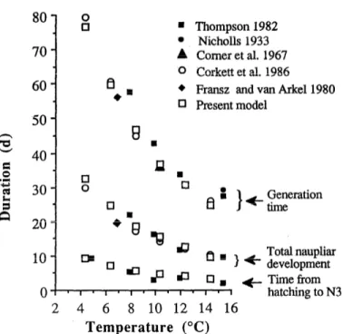
526 Carlotti and Radach 80 70 s n Thompson 1982 l Nicholls 1933 A Comer et al. 1967 0 Corkett al. 1986 et 60 50 s

+ Fransz and van Arkell980 0 Present model u n ; 40 0 .a % 2 30- q 2 q n _{20 -}

l g $

lo- [I _Is _{* ’ 1 e} _developmentTotal naupliar

q m P a 0, +Timefrom

0-k hatching to N3

2 4 6 8 10 12 14 16 Temperature (“C)

Fig. 2. Plot for CalanusJinmarchicus showing simulated and published durations of its nonfeeding period and naupliar and total development times for different temperatures and nonlim- iting food conditions.

Zooplankton model dynamics under laboratory conditions- In our model, the durations of the stages and growth curves are not parameters of the model but simulation results. These results follow the growth rate, which depends on metabolic rates that are-controlled by environ- mental factors. In Figs. 2 and 3, we compare these outputs with published results from cultures grown under stable food and temperature conditions. Corkett et al. (1986) showed that the stage durations follow hyperbolic functions of temperature, which our findings mirror. The Qlo calculated between 4 and 14°C for the times of development from spawning to N3, Cl, and adult are 3.64, 3.70, and 3.20. Mullin and Brooks (1970a) obtained a Qlo of 3.67 for the complete development of C. helgo- landicus.

Growth does not seem to be exactly exponential from N3 to C5, which means that the specific growth rate is not constant for all developmental stages. Obviously, the rate is higher for Cl to C3 than for C4 to females. The nonfeeding period before N3 and the time-dependent molting to N2 and to N3 induces a decrease in weight. The first feeding stage, N3, must recover from these losses and reach critical weight before molting into N4, which makes the N3 stage longer. Average growth rates (during the whole life from egg to adult) range from 0.08 d-l at 4°C to 0.24 d-l at 14°C which implies a Q10 for growth of 3.0. If we estimate growth rate from exponential adjustments of copepodite weights, we obtain 0.09 d-l at 4°C and 0.36 d-l at 14°C. These results are consistent with those obtained for closely related Calanus species (Vidal 1980). The modeled egg production process, which

lo2 7 10' : loo : 1 Females 0 l(1 20 30 40 50 60 70 80 I Days

Fig. 3. Plot for Calanus finmarchicus showing simulated temporal development of stage weights at different temperatures and with nonlimi ting food in a semilogarithmic scale. The weights are noted at the moment of maximum abundances during the first generation. :Lincs are exponential adjustments of copepod- i te weights.

does not account for metabolism of reserves and egg formation, is probably too simple, whereas maximum egg production under optimum food conditions and for temperatures ranging from 6 to 14°C follows the rates given by Runge ( 198 5, his figure 2).

Assumptions of the coupled model for the North Sea- We need to make assumptions concerning the vertical distribution and biology of the C. Jinmarchicus population. We propose that after ascent of the overwintering stages of the plapulation to the North Sea shelf, the population in the central North Sea remains local. We assume that C5 and adult stages present at the end of winter become active when the temperature is >4.5”C and the food concentration is ~0.04 g C m-3. In fall, when temperature and phytoplankton decline to these same values, the surviving individuals return to the over-wintering state, and their metabolism stops.

.

Initial overwintering weights of C5 and females were considered high values in the simulations, and weights above the critic:al weight of females were transformed into eggs in spring. We adopted a homogeneous distribution of zooplankton in the upper layer of 30-m depth for all stages. During winter months, we put inactive individuals in the same upper layer for model simplicity.

We assume that the available food concentration F for all the stages of the population is the mean value of the food concentration (phytoplankton and eventually other resources) in the layer occupied by zooplankton. We assume that copepods feed continuously if there is food present. Phytoplankton grazing GRAP(z, t) is propor- tional to phytoplankton concentration P(z, t) and is cal-

(7)

Table 2. Processes coupling the zooplankton submodel to the other components: NiJ- abundance; IV, - weight; 1, -ingestion; EG, - egestion; EX,-excretion; MiJ - mortality for individuals in age class j of stage i. Of the 13 stages from egg to adult, the number of age classes, NC’(i), varies with stage; Pcxt)- phytoplankton concentration; gp - P : C ratio; pM - percentage of remineralized dead phytoplankton in the water column; p,-percentage of remineralized fecal material in the water column; pz- percentage of remineralized dead zooplankton in the water column; z,,, -upper reach of zooplankton distribution; Zmi, -lower reach of zooplankton distribution.

T

F

Averaging of temperature and food in the upper layer T(t) = ’

S Zmax

Mean temperature T(z 0

Z _{max -} Zmin zmin 1

S anax Mean food available for zooplankton F(t) = P(z 0

Z _*ax- zmin Zmin

GRAZ

Outputs of the zooplankton submodel 13 NC(r) Grazed material GRAZ = C 2 Ii,jNi,j

i-l j-l FECP Total fecal pellet material

MORZ Total cadaverous material

FECP = 2 z) EG,jNi,j i-l j-1

13 NC(I)

MORZ = 2 x Mi,jN,jW,j i-l j-l

EXCR Excretion of dissolved metabolic products

13 NC(r)

EXCR = x 2 EXi,jNi,j i-l j-l

Repartition of zooplanktonic effects on the water column, Zmin I z 5 z,.,,,, GRAP Copepod grazing GRAP = GRAZS

REM1 Total remineralization REM1 = g,(REMP + REMF + REMZ) REMP Remineralization of dead phyto- REMP = pMMORP

plankton

REMF Remineralization of fecal pellets REMF = p&ECP REMZ Remineralization of zooplankton REMZ = p,MORZ

cadavers

SEDI

Formation of benthic detritus

Losses of particulate material from SEDI = (1 - p,)MORP water column + (1 - p,)FECP

+ (1 - pdMORZ

culated for each depth (Table 2). The products of zooplankton metabolism, which enter the model’s nutrient compartment (i.e. excretion, remineralized fecal pellets, and dead bodies), are evenly distributed throughout the upper layer. The remaining fecal pellets and dead bodies fall immediately to the benthic detritus compartment.

Density-dependent predation is not represented in our simulation, although our model can easily integrate this phenomen; however, we included a constant minimum mortality in all simulations.

North Sea simulations-The coupled model was used to show the importance of differential dynamics of stages as related to the environment. First, runs were performed with the annual plankton dynamics in the central North Sea at the position of the ocean weather ship (OWS) Fami-

ta (57”N, 3”E), and the results were compared with those of Radach and Moll(1993) for 1984 (see their figure 23). The goal was to see how the population is driven by physical forcing. Second, we simulated the spring plankton dynamics in the northern North Sea at the position of the Fladen Ground Experiment (58’5 5’N, O”32’E) in spring 1976 (see Radach et al. 1984) with the same model. The goal here was to study the link between phytoplankton and development of the zooplankton population. Be- cause detritus production in this area is important during this period, we introduced pelagic detritus in our model to attempt to reproduce the observations made during FLEX’76.

Equations and numerical scheme- For the biological part of the model, the system of equations consists of two

(8)

Table 3. Differential equations for pelagic detritus and new processes. Detritus concentration PD(z,

t);

turbulent diffusion coefficient--A,; phytoplankton sinking velocity w,; detritus sinking velocity-w,; detritus remineralization rate--n; height of water column--H. Other abbreviations as in Table 2.

PD dPD(z, ~

_at

t)

= DIFD - SIND + MORD + FEPD + n4OZD - GRAD - REMD POC dPOC(z.

t)

=- amt) + apw,t) -

at at at

POC Particulate organic C POC(z,t) = P(z,t) + PD(z,t)

Zmax

F Mean food available for zooplankton F(t) == 1

Z - Zmin

S

POC(z,

t)

max Imin

Zooplankton and phytoplankton equations given in Table 2 Pelagic detritus equation

DIFD Turbulent diffusion of pelagic detritus

SIND Sinking of pelagic detritus

MORD Flux of dead phytoplankton MORD = prAMORP FEPD Flux of fecal pellets FEPD = p,FECP MOZD Flux of zooplankton carcasses MOZD = p,,MORZ GRAD Copepod grazing on pelagic detritus GRAD = GRAZ- PD(z, 0

F(t) REMPD Remineralization of pelagic detritus REMPD = r,,PD Nutrient equation

REM1 Total remineralization REM1 = REMPD Benthic detritus equation

J%(z) Flux condition at the boundary for Fp(lr) = - wsP(z,t)H - w,PD(z,t), phytoplankton and detritus

nonlinearly coupled second-order partial differential equations that simulate changes in the local concentrations of phytoplankton and phosphate, two ordinary first- order equations for light (Beer’s equation) and benthic detritus (Radach and Moll 1993, part 2), and a subsystem of 26 ordinary and nonlinear first-order differential equations for zooplanktonic stage dynamics and growth (Car- lotti and Sciandra 1989, their table 2). The processes linking the zooplankton submodel to Radach and Moll’s (1993) model are presented in detail in Table 2. The values of the parameters for the copepod submodel are explained above. Other parameters adopt the values given by Radach and Moll(1993, their table 1) for their annual simulation. When we simulated the spring dynamics at the FLEX’76 station, we changed only the depth (150 m) and the C : Chl ratio, which was calculated to be 15 during FLEX’76 (Radach et al. ICES CM1980K3). For the FLEX’76 simulations, the additional equations and processes relating to the model’s pelagic detritus compartment are presented in Table 3.

The equations for light, phytoplankton, phosphate, and detritus are solved numerically by a combination of ex- plicit difference schemes (see Radach and Moll 1993) with a time step of 75 s, and the zooplankton subsystem is

solved by fourth-order Runge-Kutta numerical integration with a time step of 3 h. The runs were performed on a Siemens computer (789OF) with the MSF system. For a yearly simulation, one run lasted 8 min. For the FLEX’76 simulations, the copepod submodel was called at each integration step of the main model (every 75 s), with one run lasting 30 min.

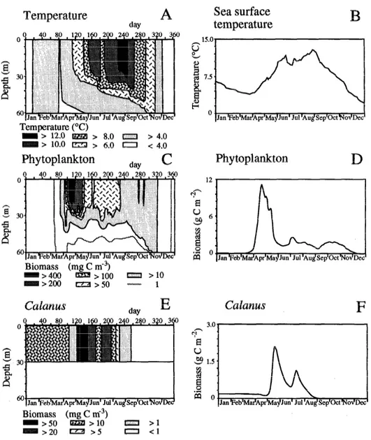
Results

Annualplankton cycle-Radach and Moll(1993, figure 23) presented concepts, results, and validations of the physical and biological parts of the model with zooplankton forcing and gave the annual physical and biological dynamics at the OWS Famita site for 1984. For the same year, we present the simulation made with a dynamic population of 15’. jinmarchicus. The simulated upper-layer temperature (Fig. 4A,B) began to increase at the end of March and reached 13°C at the end of August. A strong summer storm at the end of June broke up the thermocline and supplied the upper layer with nutrients. The thermocline formed again in July and progressively erod- ed in fall. The spring increase of temperature and the

(9)

i

Temperature

A

day

Sea surface

temperature

15.0. u^ ’ e i!i _{@ 7.5}: Ii : G ’ 0.

Jan ‘Feb’Mar’Apr’MajJun’ Jul’Au~Sep’Ckt’No~Lk

Temperature (“C) m > 12.0 Em > 8.0 0 > 4.0 > 10.0 [123 > 6.0 0 < 4.0

Phytoplankton

day

C

Phytoplankton

Biomass (mg C m-“) ->400 ->100 m >lO >200 czi>50 - 1

Calanus _day

E

Calanus

Biomass (mg C tri3)

- >50 Em >lO I. >l

>20 m >5 I cl

Fig. 4. Annual standard simulation. Shown are simulated profiles of temperature and evolution of upper-layer temperature and simulated profiles and integrated biomass of phytoplankton standing stock and of Calanus finmarchicus in 1984 for the OWS Famita site in the central North Sea. Initial densities of C. Jinmarchicus stages are 900 C5 m-2 and 450 females m-2.

subsequent water-column stability induced the development of a phytoplankton bloom, which was followed by an increase in zooplankton (Fig. 4C-F). Food for C. jinmarchicus copepodites, in the form of phytoplankton concentrations >50 mg C3 (Fransz et al. 199 la), was found in the upper 30 m from April to mid-August. We assumed an even distribution of copepods in the upper 30 m. The initial overwintering stocks were composed of 30 C5 and 15 adult females m-3, which resulted in an integrated biomass of 0.175 g C m-2. This value was within the range of observed biomasses of C5 and females at the end of winter in the North Sea (Williams and Con- way 1980). We did not study the dynamics of the overwintering population, which occurs in North Atlantic deep waters and arrives in the northern North Sea at the end

of winter (Fransz et al. 199 la). The simulated biomass of Calanus in the surface layer from January to the beginning of April was artificial; for simplicity, we supposed the overwintering stock constant and inactive in the upper layer. When the copepods became active at the beginning of April, their biomasses began to decrease (Fig. 4E,F) because of a weight decrease of individuals subject to food limitation. The biomass then increased exponentially in the beginning of May, 4 weeks after the increase of phytoplankton (Fig. 4C,D). Calanus biomass and abundances decreased in the second part of May, when phytoplankton biomass decreased.

During summer, each meteorological event breaking the thermocline influences planktonic distributions and populations. The storm at the end of June eliminated the

(10)

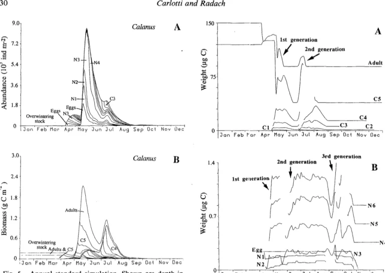
530 Carlotti and Radach N3- N2- Calanus

A

2.4 A % u 1.8 oJ3 CA 3 1.2 E 0 .+ a 0.6 0 Calanus B

Fig. 5. Annual standard simulation. Shown are depth-integrated and cumulative abundances and biomasses of the stages of Calanus jinmarchicus. Simulation begins with an overwintering stock of 900 C5 m-2 and 450 females m-2.

thermocline (Fig. 4A), permitting an input of benthic regenerated nutrients, followed by a new development of phytoplankton and zooplankton (Fig. 4C-F). In fall, the concentrations of phytoplankton stayed low due to mixing of the entire water column. Because Calanus is unable to catch enough food when phytoplankton concentrations are low, there is no population increase in fall. We did not model the sinking of the population in deep waters, so the population starves in the upper layer and disap- pears.

The copepod population model simultaneously provides the time variations for numbers of individuals (Fig. 5A) and for biomasses of each stage (Fig. 5B). Initial concentrations of C5 and adult females were negligible in numbers, but not in biomass. Two complete distinct generations developed throughout the year, one beginning in April and the other in May. The peak of biomass in May was mainly due to the high proportion of C5 and adults of the first generation. Figure 5B clearly illustrates the overlap between the first and second generations. The second generation, present from the first spawning in May to the adults in August, seemed to develop slowly and had a high mortality rate (Fig. 5A). The phytoplankton

1st generation

A

;J i?neration *dult 0 3rd generation 2nd generation - I

Fig. 6. Annual standard simulation. Shown are simulated mean body weights for copepodite and adult stages and for eggs and the six naupliar stages. Curves end when the abundance of individuals of each stage is < 1% of the total population for naupliar stages and ~0.5% for copepodite and adult stages.

peak in July permitted a new growth period for the second-generation copepodite stages, and some females produced a relatively small number of eggs to give a third generation in September (visible mainly in the growth curves).

Overwinterilg C5 and adults had stable weights from January to the beginning of April. In our model, copepod metabolism is not activated at such low temperatures and phytoplankton concentrations (Fig. 6A). We chose high winter weights for C5 and adults to represent reserves used for egg production. In April, the individuals became active and at lirst lost weight due to insufficient phytoplankton concentrations; thereafter, they grew by feeding on the phytoplankton bloom, and the adult females produced eggs. One hypothesis of our model was that egg weight (Fig. 6B,) stayed constant, but weights within stages varied in sevel-al ways.

It is important to discriminate between the two phe- nomena that influence the evolution of mean weight in a stage: one phe:lomenon concerns the inflow and outflow of individuals passing through the stage, and the other

(11)

Phytoplankton c

N3

Calanus B 9.0.

Calanus D

(High overwintering stock) 7 2, _(Delayed_arrival

of overwintering adults) 5.4 3.6 , 1 1.8

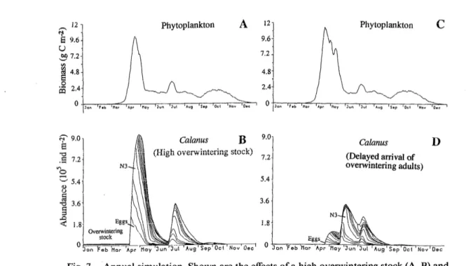
Fig. 7. Annual simulation. Shown are the effects of a high overwintering stock (A, B) and

of a delayed ascent of overwintering individuals (C, D) for the depth-integrated biomass of

phytoplankton and depth-integrated and cumulative stage abundances of Calanus Jinmar- chicus. The simulation with a high overwintering stock begins with 9,000 C5 m-2 and 4,500 females m-2; the simulated delay begins with the same densities as in Fig. 5.

phenomenon refers to the growth of individuals within the stage. Newly hatched individuals did not feed before stage N3 and thus lost weight during Nl and N2. The individuals of the first cohort, produced by over-wintering individuals, grew rapidly; the eggs spawned in April became adults 30 d later. The second cohort mostly started in May and spread until the beginning of August; some precocious individuals reached the adult stage as soon as the end of June. By combining this information on growth with the dynamics of individuals, we can affirm that most individuals had a lower growth rate during the naupliar and copepodite phases with a low phytoplankton concentration in June; subsequently, the copepodite stages resumed exponential growth with the rise of phytoplankton in July. Individuals of a third cohort were produced in July by the precocious females of the second generation, and their development was concomitant with individuals of the second cohort. There were some individuals of a fourth cohort in September, but they developed no farther than stage N6 because of the lack of food and the severe decrease in temperature. Growth curves stopped because of the death of individuals, except for C5 and adults who entered over-wintering status.

We investigated the effect of the initial overwintering stock on dynamics by starting with initial densities of 900 C5 and 450 adult females m-3- 10 times higher than in the basic simulation. These high initial copepod biomasses and densities changed the plankton dynamics in spring (Fig. 7A,B). Although this overwintering stock remained negligible in terms of total individuals, it was considerably higher in terms of biomass, with a value of 1.7 5 5 g C m-2. During the exponential increase of phy-

toplankton biomass, zooplankton stock fell to 1 g C m-2, then increased to 3 g C m-2 until 10 May, thus producing the same biomass as the basic simulation. Egg production lasted longer than 1 month (from the beginning of April to mid-May; Fig. 7B), with a first peak due to the initial females and a second very wide peak originating from the initial C5. The growth of the early individuals of the first cohort was fast during the naupliar stages, then slowed in stages C2 and C3 during mid-April because the resources needed to complete their development had been considerably reduced (Fig. 7A). Most of the individuals born later stopped their growth in the previous stages, which led to high biomasses in C2 and C3 when the biomass peaked in May. Phytoplankton biomass stayed between 1 and 2 g C m-2 in May and June, and lower competition for food among the living copepods permitted the survivors to resume their growth. The females spawned again after 15 May and produced a first cohort of second-generation individuals in May-June, whereas individuals whose growth had stopped in a naupliar stage reached the adult stage at the end of June and initiated a second cohort of the second generation in July.

The timing of the spring ascent of overwintering individuals also influences subsequent plankton dynamics (Fig. 7C,D). A 5-d delay in April for the Calanus ascent did not greatly affect the number of individuals in the first generation when compared with the basic simulation (see Fig. 5), but the delay did shift the appearance of females in the first generation. These females matured after the end of the bloom, and recruitment of the second generation was considerably reduced. At the beginning of July, the increase in phytoplankton permitted new egg

(12)

532 Carlotti and Radach production; in addition, all stages resumed growth, which

had been food limited during the last weeks of June. Plankton bloom dynamics in spring-To understand in detail the dynamics of the pelagic ecosystem during the crucial spring period, we simulated the dynamics of the ecosystem from 5 April to 6 June 1976 and compared them to the data obtained during FLEX’76. The physical model was slightly adapted to the Fladen Ground area, thus the bottom is 150 m deep. The main features of the spring plankton bloom in the northern North Sea in 1976 that we wanted to simulate are presented by Radach (1980, his figure l), Radach et al. (1984, their figure l), and Krause and Radach ( 19 89, their figure 2).

was maximal between 28 May and 5 June, with a value in the range of the FLEX’76 observations. The profiles of phytoplankton and zooplankton show an apparent gap in the food supply for zooplankton; this gap may be filled by detritus, as indicated by the POC concentration (Fig. 8D).

In our model runs, the initial concentration of phytoplankton was set at 0.3 mg C m-3 at the surface and reduced by 1.66% m-l at a depth of 60 m (Gassman and Gillbricht 1982). We assumed that a population of C. finmarchicus arrived in the FLEX’76 area on 22 April via

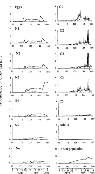
currents (see figure 1 of Radach 1983), but remained iso- lated afterward. The initial population had no eggs and no nauplii Nl-N5, 1,000 N6,400 Cl, 70 C2, 70 C3,70 C4, 80 C5, and 140 adults m-3 (Krause and Trahms

1983), for a total biomass of 0.0356 g C m-3.

The first simulations, which took into account only the dynamics of the phytoplankton and zooplankton, did not reproduce the observations from FLEX’76 (Krause and Trahms 1983). The phytoplankton bloom was large and Calanus quickly grazed it down, but the copepodite stage abundances obtained in the simulation were < 20% of the numbers observed in May. Complementary simulations with higher initial numbers of individuals did not change the results; the high initial Calanus biomass quickly grazed all the phytoplankton, resulting in a low phytoplankton standing stock in May and a high mortality of zooplankton. This result was similar to results obtained in the yearly simulations. We inferred that the development of the observed C. finmarchicus population was possible only if there were a complementary source of nutrition, either detrital remains or microzooplankton. Therefore, we added a pool of pelagic detritus to our model because Gass- mann and Gillbricht (1982) had measured high levels of pelagical detritus in the upper 30 m during FLEX’76 (their figure 1). All the processes that enriched the benthic pool of detritus in the previous model (Fig. 1, i.e. phytoplankton mortality, zooplankton excretion, fecal pellet production, and death of copepods) supplied a pool of detritus to the water column. This material sank at a rate of 2 m d-l in this new version of the model. The new processes are described in Table 3.

At the end of the simulation, when the zooplankton biomass became high in the upper 30 m, phytoplankton biomass was found primarily in deeper parts of the upper layer. Strong grazing pressure eliminated phytoplankton cells in the shallow part of the upper layer and diminished self-shading. In our simulation, the copepods do not migrate. Therefor’:, phytoplankton and detritus were not grazed below the thermocline and provided a high level of POC after 20 May below 30-m depth. The abundances of copepodite :;tages in the water column (Fig. 9) are consistent with observations by Krause and Trahms (1983), but the simulated numbers for the nauplii are twice as high as their observations. Females present on 22 April produced the first peak of eggs. The development of these individuals can be followed through stage C5, but they do not reach adult stage before the end of the simulated period. The adult females, who had been the initial individuals in stages N6-C5, spawned eggs continuously during a month-long period after 27 April. These eggs furnished the high densities of individuals in stages Cl-C5 at the end of the FLEX’76 period and were of the same magnitude as densities observed by Krause and Radach (1980). The last peak of eggs was produced by females from the development of the initial N6 cohort.

Growth curv.es (Fig. 10) clarify this interpretation of the dynamics. When the population arrived in the area, only the N6 nauplii grew because they could feed on lower concentrations than could the other copepodite stages. By contrast, the initial copepodite stages lost weight during the first days oY the bloom, then grew normally. From 22 April to 19 May, the mean weight of females fluctuated slowly because of continuing egg production. The copepodite growth curves fluctuated because there were successive cohorts produced by females from initial densities in different stages. Weight of initial females decreased as they produced eggs. The eggs spawned by these females generated a distinctive cohort, with rapid naupliar growth from 24 April to 9 May (Fig. 10B) followed by a slow growth in the copepodite phase from 9 May to the beginning of June (Fig. IOA). The cohort produced by the initial group of N6 nauplii developed through the copepodite stages fr,om 29 April to 25 May. These individuals became adults after 25 May and produced the last peak of eggs seen in Fig. 9.

The simulated temperature profiles during the FLEX’76 period exhibited stratification in May and June (Fig. 8A). Temperatures progressively increased in the upper layer

from 6°C on 5 April to 9.5”C in June.

Discussion

The phytoplankton bloom in the simulation took place Comparison of simulation and FLEX’76 data-The between the end of April and 10 May (Fig. 8D). Detritus simulation of l:he thermal stratification of the water col- (Fig. 8C) was abundant mainly when the phytoplankton umn during FLEX’76 shows an increase in the upper- concentration exceeded 200 mg C m-3, and its maximum layer temperalure (Fig. 8A) and is consistent with the concentration was deeper than the 30-m layer. The C. observations CI f Soetje and Huber (see figure 2 of Krause finmarchicus biomass (Fig. 8E) increased after 8 May and and Radach 1989).

(13)

Temperature

96 106 116 126 136 146 156 0

Phytoplankton

96 106 116 126 136 146 156

Detritus

_&Y

C

96 106 116 126 136 146 156

April ’ _May ’ June

Temperature (“C)

m > 9.5 m> 8.5 [3> 7.5 * - * 7.0 > 9.0 m > 8.0 - 6.5

Biomass (mg C n-i3 )

>400 ~>I00 F”J>lO --- 1 >200 El> 50 - 0.1

Particulate organic carbon D

&Y 96 106 116 126 136 146 156 0 Calanus day

E

96 106 116 126 136 l& 156 0 dl 24 3 1’5 25 May

Fig. 8. Standard FLEX’76 simulation. Shown are simulated profiles of temperature, phytoplankton, pelagic detritus, particulate organic C, and Calanusfinmarchicus during FLEX’76. The population of Calanus begins with the stage densities (per m2) observed by M. Krause (pers. comm.) on 22 April: 1,000 N6; 400 Cl; 70 C2; 70 C3; 70 C4; 80 C5; and 140 adults.

The simulated biomass profiles for phytoplankton and the lower grazing pressure on phytoplankton when Cal-

detritus (Fig. 8B,C) can be compared with the observed anus has two available food sources; we assume that co- distributions of active chlorophyll pigments and phaeo- pepods feed equally on phytoplankton and detritus. In phytin pigments, respectively (figures 2 and 4 of Radach reality, copepods probably prefer fresh living phytoplank- et al. ICES CM1980K3; figure 1 of Radach et al. 1984; ton when it is present; if it is unavailable, they switch to figure 2 of Krause and Radach 1989). Our simulated phy- detritus. During FLEX’76, ingestion by zooplankton ex- toplankton biomass starts with an exponential growth ceeded production of phytoplankton (Williams and Lind- that is coincident with the observed bloom of phyto- ley 1980a; Daro 1980; Radach et al. 1984). Other me- plankton. The maximum concentrations of simulated sozooplanktonic species (e.g. Thysanoessa inermis, Oi- phytoplankton are higher than those observed because thona sp.) also were observed before the spring bloom

our simulated grazing rate is too low for the first days of (Williams and Lindley 1980a; Krause and Trahms 198 3) the bloom. We also note that the phytoplankton bloom and may have acted as a fine but decisive control on the lasts longer when we include pelagic detritus because of phytoplankton at the beginning of the bloom (Lindley

(14)

96 112 128 144 160 96 112 128 144 160 4 Nl 1 96 112 128 144 160 4

1

N2 0 96 112 128 144 160 4] N3 96 112 128 144 160 4 1 N4 96 112 128 144 160 0 96 112 128 144 160 4, N5 4 , Adults 2

I

0 96 112 128 144 160 4

1

N6 2d - 0 Inrllrr,-rr* j&/-&y& r, 7r4?=6+mTr,,,r., 96 112 128 144 160 7 I 1 I I 1 r , 5 13 21 2’ 7 I.5 23 3 8

April May June

Carlotti and Radach

96 112 128 144 160 96 112 128 144 ‘160 96 112 128 144 160 4 1 c5 0 -- Ill-m 76 96 112 128 144 160 20 , Total population , 96 112 128 144 160 7 I , 1 I , , , 5 13 21 2 7 15 233

April May Ju:

Fig. 9. Standard FLEX’76 simulation. Shown are simulated depth-integrated abundances of individuals of Calanusjinmar- chicus stages during FLEX’76 for the water column (thick lines). Data for the naupliar and copepodite stages (thin lines) are from Krause and Trahms (1983).

and Williams 1980). There was high microbial activity (Gieskes and Kraay 1980), and these organisms also could have grazed on the phytoplankton biomass. The sedimentation of detritus occurred mainly after 4 April in our simulation (Fig. SC), which coincides with timing in reported observations (see figure 4 of Radach et al. ICES CM 198O/C3). The abundant total POC in the upper layer from 28 April to 21 May in our simulation (Fig. 8D) is consistent with the findings reported by Gassmann and Gilbricht (1982, their figure l), although POC concentration decreased as early as 10 May.

The approx:.mation of a homogeneous distribution of Calanus in the, upper 30 m (Fig. 8E) is essentially correct at the beginning of FLEX’76, but not after mid-May (see figure 5 of Krause and Radach 1989). The simulated development of C. jinmarchicus nauplii and copepodites (Fig. 9) is chronologically similar to the observations of Krause and Trahms (1983), and the simulated abundances of copepodite and adult stages have the proper magnitude. However, our simulations suggest that the in situ naupliar densities must have been greater than those counted by Krause and Trahms (1983, their figure 4), based on the assumption of local population dynamics. The review by Fransz et al. (199 la) suggested that the population in the Fladen Ground is subject to advection and that there is an import of copepodites. Our model densities, begi nning 22 April, simulate densities observed by Krause and Trahms (1983) at the end of May.

Both simulated growth and development suggest that no more than one generation could occur during the FLEX’76 study period and that growth of the population also could have been possible based on local food supply. Gamble (1978, his figure 2) presented the growth of the mean dry weight of the subgroup of C4, C5, and adults from 25 April to 10 May and noted an “inversion of stages” on 10 May marked by a decrease of this mean weight. Our simulation (Fig. 10) indicates that such an inversion probably was caused by the simultaneous pres- ence of several cohorts.

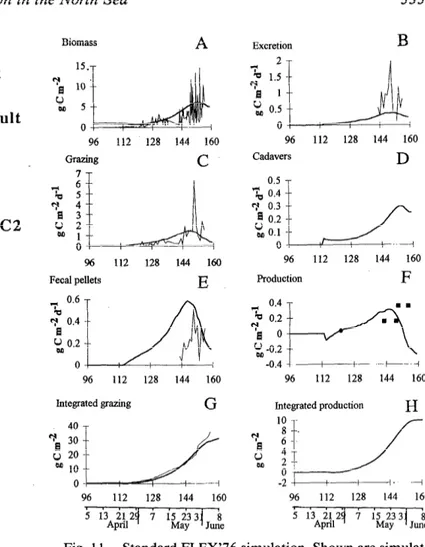
The simulated C. finmarchicus biomasses (Fig. 11 A), which are the combined individual growth and abundances, are comparable to those observed by Krause and Radach ( 1980). Daro ( 19 80) studied C. Jinmarchicus grazing in the upper 40 m from the end of May to the beginning of June and calculated production from respiration data and egestion for the same period (see Daro 1980, table 3). Our simulated ingestion rate (Fig. 11C) is corn- parable to Dare’s 23 May data, but our ingestion rate decreases in J’une, whereas Daro observed a maximum grazing of 2.5 g C m-2 d-l during this time. Our simulated production of’ fecal pellets (Fig. 11E) is of the same order as the simulations and observations in June, but is over- estimated by 1 he simulations in May. Simulated excretion is lower than the estimated respiration losses (Fig. 11B). Daily loss of matter by death is also an important process in the biomass balance of the population (Fig. 11D). The simulated productivity at the beginning of May is equal to that estimated by Fransz and van Arkel(l980). During the last 10 d of May, the simulated productivity is higher than Daro’s (1980) values. In June, however, the simulated productivity falls, whereas Daro calculated a net production of 360 mg C m-2 d-l. Our decrease in the simulated ne’; production is correlated with the decline of the growth rate of older copepodites (Fig. 10A) and the decrease in egg production (Fig. 9) because of unfa- vorable feeding conditions in the upper 30 m (Fig. 8D). Fransz (ICES, CM1980/C3) also found that the growth rate of the largest copepodite stages was low at the end of FLEX’76 and that the C5 “hesitated to become adult.”

The time-integrated rates for phytoplankton production, copepod grazing, fecal pellet production, and ma-

(15)

Production in the North Sea

First cohort Second cohort

Adult C5 96 160 -I I 5 I I 5 13 21 29 7 April

B

First cohort Second cohort

i

/k----J

Iv4

96 160

-I I I I I

5 13 21 29 7 April

Fig. 10. Standard FLEX’76 simulation. Shown are simulated mean body weights for copepodite and adult stages and for eggs and naupliar stages.

terial excreted by Calanus are also calculated by the model. For the FLEX’76 period, the simulated primary production reaches 49.4 g C m-2, which is in the range of production estimated by several investigators (see Ra- dach et al. 1984). The simulated integrated grazing (Fig. 11 G) is significant after 16 May and reaches a cumulative value of 30.85 g C m-2 at the end of the simulation. Only 8.3 g C m-2 were grazed from phytoplankton, illustrating the importance of detritus. This grazing value is lower than all values estimated by Radach et al. (1984), except when they assumed the amount of grazing to be 10% of the biomass. The simulated secondary production of C. jinmarchicus during FLEX’76 (Fig. 11H) reaches 10 g C

mm2.

Efect of diel migration at the end of FLEX’76-The simulated biomass of the entire population reaches a maximum before the end of the FLEX’76 period, there is then a net decrease, resulting in a stock of 5 g C m-2 at the end of FLEX’76. This decrease was not observed

Biomass 15. 3 a lo w 00 5 0 96 112 128 144 160 Grazing _C 7-r w 2 om 1 0 96 112 128 144 160 Fecal pellets _E - 0.6 b 3 0.4 a t 0.2 96 112 128 144 160 Integated grazing _G 96 112 128 144 160 5 I , I , , , I

5 13 21 2 April 7 ‘hi; 3 hufe

Excretion B 2 7 ,” 1.5 'a 1 k 0.5 0 96 112 128 144 160 Cadavers _D 0.5 -i& 0.4 5 3 0.3 a : 0.2 0.1 0 96 112 128 144 160 Production F v a w M 96 112 128 144 160 Integrated production _H 96 112 128 144 160 3 I I I , , , I 5 13 21 2 April 7 1523 3 Juk

Fig. 11. Standard FLEX’76 simulation. Shown are simulated depth-integrated biomasses of Calanusfinmarchicus (A) and the processes of excretion (B), grazing (C), production of dead bodies (D), and fecal pellets (E) (thick lines). Data (thin lines) are from Krause and Radach (1980) for biomass and from Daro (1980) for processes. Simulated production (F’) of C. jnmarchicus (line) is compared with the estimates of Fransz and van Arkel(l980) (0) and Daro (1980) \. The simulated cumulative grazing (thick line) is compared with grazing calculated by Ra- dach et al. (1984) (thin line) with the “POC limited approach” (G). Simulated secondary production (H) during the period of FLEX’76 is calculated as grazing minus fecal pellet production and excretion.

in reality (Krause and Radach 1980) but is caused by food-limited grazing after 27 May (Fig. 1 lC), which di- minishes and stops growth of individuals (Fig. 10A). Krause and Radach (1989) showed that all the copepodites carried out diel vertical migrations after 15 May, but never before this date. The mean depth of the center of gravity of the copepodite and adult stages of C. jinmarchicus was 21 m during the algal bloom; thus, the assumption of an even distribution of C. Jinmarchicus in the upper 30 m is largely correct for this period. After the algal bloom, the mean depth of the center of gravity was 34 m, and the copepods carried out diel vertical migrations.

(16)

Particulate organic carbon A

96 106 116 126 136 146 156

April ’ _May ’ June

Calanus 96 106 116 126 136 146 156 0

Biomass (mg

->400 ta>lO

>200 El>50 C ti3) c-J>10 --- 1 - 0.1

Population biomass

April ’ ’ June April

‘3 1:

May

31

June Fig. 12. Simulation during spring with migration. Shown are simulated profiles of particulate organic C and Calanusjinmarchicus during the period of FLEX’76, and the integrated biomass of C. finmarchicus. The initial conditions (stage abundances and weights) are identical to those of the standard FLEX’76 simulation in Fig. 10. The migration is affected after 15 May from O-30 m to 20-50 m. The figure shows only one position per day at noon, but the organisms actually migrate following a periodical sinusoidal function.

grated from O-30 m at night to 20-50 m during the day (Fig. 12B). The biomass of Calanus then increased until the end of FLEX’76 (cf. Figs. 12C and 11A). The individuals could have fed in deeper regions (cf. Figs. 12A and SD) and their growth continued. This result suggests that migration can give a metabolic advantage when the total food sinks to deeper layers. Daro (1980) noted the strongest diel vertical migrations when the available food became scarce.

Annual cycle of Calanus finmarchicus- Williams and Lindley (1980b) suggested that the success and strength of the overwintering population is fundamental to the strength of the developing spring cohorts. Comparing our annual simulations that begin with different overwintering copepod biomasses or with different dates of ascent of overwintering stages (Figs. 5,7), it is obvious that initial conditions influence the dynamics of both phytoplankton and Calanus populations. Our simulations show that a too high initial biomass of overwintering zooplankton can have a negative effect on the resulting population.

At the beginning of the spring bloom, development of the first generation of C. jnmarchicus lasts 1 month if it is initiated by a normal overwintering stock (Figs. 5,7D). During this bloom period, the limiting growth factor is temperature, which increases slowly in the upper layers.

Pedersen and Tande (1992) showed that in the Barents Sea the naupliar stages spawned by overwintering females have different optimum temperatures for their growth; these optimum temperatures are linked with the spring increase in temperature. Such a phenomenon also may play an important role in the North Sea, as well as in the timing of ontogenic vertical migration of over-wintering individuals to the surface layers. The highest population biomass is produced by the last stages of the first generation, and the highest abundances occur with the first stages of the second generation, as observed during FLEX’76 (Krause and Trahms 1983; Krause and Radach

1980). The highest grazing pressure from C. Jinmarchicus comes from the last stages of the first generation, which reduces the phytoplankton stock in May. Therefore, the simulated blaom is limited by nutrients at the end of April, as in the simulation made by Radach and Moll (1993, their figure 23) with zooplankton forcing, and then by the grazing of late copepodites of the first generation. The success of the first generation produced by overwintering female:; of Calanus can play a role in bloom limitation (Fig. 7A,B).

In the Nortll Sea, the peaks of phytoplankton are short- er (Radach et al. ICES CM1980K3) than in our annual simulation. Obviously, grazing by C. Jinmarchicus that occurs mainly, in May cannot be the only process limiting

(17)

the phytoplankton bloom. Other grazers may play an important role during the first weeks of the bloom and probably are replaced afterward by the first generation of C. finmarchicus. Fransz and Gieskes (1984) suggested that

microzooplankton play a role both as grazers of phytoplankton and as a food source for zooplankton. When we added a pelagic detritus compartment to the FLEX’76 simulations, the simulated stage abundances and biomasses finally had the right magnitude. We may reason- ably assume that there is a link between microbial activity and detritus, and that copepods feed not only on detritus, but also on microbial organisms. An additional improve- ment to the model would be to add a microzooplankton compartment.

The growth curves for each stage are essential to clearly understand the stage dynamics. Our basic simulation shows a weight decrease in overwintering stages before the spring bloom, as observed by Tande (1982). A comparison between the first and the second generations (Fig. 6) reveals that the first is limited by temperature, whereas the second is clearly limited by food in June and July. The growth curves of copepodite and adult stages show that individuals of the second generation at the end of . _{June and the end of July are the last C5s and adults of} the year. Several workers (see Fransz et al. 199 1 a) have suggested that copepodites and adults sink into deeper layers as early as July, constituting the next overwintering population. This interesting result shows that growth, development, and life strategy must be understood together in relation to the environment.

Our model also could be used to study regional differ- ences. C. finmarchicus is not the dominant copepod species after July in the North Sea, but the model provides some interesting results. The storm at the end of June induced a diffusion of bottom-regenerated nutrients into the upper layer and decreased sea-surface temperature; after this storm, phytoplankton biomass was between 50 and 100 mg C m-3, and zooplankton biomass was between 10 and 20 mg C m- 3. These ranges are the same as those estimated by Peterson et al. (199 1) for the second part of August in the Skagerrak.

Comparison of simulations with and without zooplankton forcing (Fig. 4; figure 23 of Radach and Moll 1993) shows that forcing influences phytoplankton dynamics differently than it does zooplankton dynamics. With forcing, the phytoplankton peak is lower and narrower because of high zooplankton biomass estimated from CPR (continuous plankton recorder) data. Moreover, the small peak of phytoplankton following the storm of the end of June seems to be shifted toward mid-July and is very low due to strong grazing pressure from the high biomass of zooplankton. In the simulation of zooplankton dynamics, the biomass of Calanus decreases after the spring bloom, so that regenerated nutrients that go into the upper layer are utilized for phytoplankton production, which is not immediately grazed. This summer production permits copepodite stages of the second generation to resume growth (Figs. 5, 6). In fall, the phytoplankton standing stock is evenly distributed over the entire water column, and concentrations are < 50 mg C m-3. Copepodites can-

not develop in such situations. This result suggests that the decay of C. finmarchicus in fall and its replacement by other species could be due to changes in the physical environment rather than competitive pressure from other species.

Note that the dynamics of the Calanus population changes considerably when we use a high overwintering stock of C5s and females (Fig. 7A,B), but the evolution of phytoplankton standing stock in summer and fall is similar (cf. Figs. 4D and 7A). In the standard annual simulation, total phytoplankton production is 146.92 g C m-2 yr-* from April to October, of which 21.04 g C m-2 yr-l is grazed. If we include the production of fecal pellets and excretion, we obtain production values of - 10 g C m-2 yr-l, which is in the range of secondary production values presented by Fransz et al. (199 la) for the northern North Sea. During the whole year, 14.3% of the phytoplankton production is grazed by C. finmarchicus. These values are high compared to other estimates (Niel- sen and Richardson 1989) because C. finmarchicus has no competitors for grazing phytoplankton in our model. From a different site, Aksnes and Magnesen (1983) estimated C. finmarchicus grazing to be between 25 and 90% of the primary production. Joiris et al. (1982) presented a carbon budget for the Belgian coastal zone (see their table 1). They obtained a primary production rate of 170 g C mm2 yr-l and a zooplankton grazing rate of 80 g C m-2 yr- l. Their biomasses of detritus and mi- croheterotrophic activity also were high in the ecosystem off the Belgian coast.

Conclusion

Because we used a 1-D water-column process model, we were able to use a detailed biological approach of population dynamics coupled with physical and biological variations in the water column during the year. The links between individual behavior and population dynamics of the copepod model allowed us to form a relationship between physiological rates and the evolution of zooplankton biomass. In our model, the development of C. Jinmarchicus adjusts itself to the dynamics of its food supply.

The threshold of food concentration above which copepods can survive seems to be an essential parameter at the beginning of the bloom and at the end of summer when the thermocline deepens. Copepod abundance depends on physical processes in the water column and on biological processes, such as phytoplankton growth and sedimentation. Following the work of Mullin and Brooks (1976) and Fernandez (1979), we established a lower threshold for naupliar stages than for copepodite stages. This phenomenon could be important at the beginning of the bloom when food concentration increases.

Our model allows us to reproduce realistic time lags between the availability of a new resource and the following growth of the population. The simulations show that the zooplankton population clearly misses the phytoplankton bloom if it is brief. Two complete generations