HAL Id: hal-01045219
https://hal.archives-ouvertes.fr/hal-01045219
Submitted on 24 Jul 2014
HAL is a multi-disciplinary open access
archive for the deposit and dissemination of
sci-entific research documents, whether they are
pub-lished or not. The documents may come from
teaching and research institutions in France or
abroad, or from public or private research centers.
L’archive ouverte pluridisciplinaire HAL, est
destinée au dépôt et à la diffusion de documents
scientifiques de niveau recherche, publiés ou non,
émanant des établissements d’enseignement et de
recherche français ou étrangers, des laboratoires
publics ou privés.
Optimization of starshades: focal plane versus pupil
plane
Rémi Flamary, Claude Aime
To cite this version:
Rémi Flamary, Claude Aime. Optimization of starshades: focal plane versus pupil plane. Astronomy
and Astrophysics - A&A, EDP Sciences, 2014, pp.1-10. �hal-01045219�
Astronomy & Astrophysics manuscript no. Starshade ESO 2014c July 24, 2014
Optimization of starshades: focal plane versus pupil plane
R. Flamary
1and C. Aime
1Laboratoire Lagrange, UMR CNRS 7293, Université de Nice Sophia-Antipolis, Observatoire de la Côte d’Azur, Parc Valrose, 06108 Nice, France
e-mail: [email protected], [email protected]
July 24, 2014
ABSTRACT
Aims.We search for the best possible transmission for an external occulter coronagraph that is dedicated to the direct observation of
terrestrial exoplanets. We show that better observation conditions are obtained when the flux in the focal plane is minimized in the zone in which the exoplanet is observed, instead of the total flux received by the telescope.
Methods.We describe the transmission of the occulter as a sum of basis functions. For each element of the basis, we numerically
computed the Fresnel diffraction at the aperture of the telescope and the complex amplitude at its focus. The basis functions are circular disks that are linearly apodized over a few centimeters (truncated cones). We complemented the numerical calculation of the Fresnel diffraction for these functions by a comparison with pure circular discs (cylinder) for which an analytical expression, based on a decomposition in Lommel series, is available. The technique of deriving the optimal transmission for a given spectral bandwidth is a classical regularized quadratic minimization of intensities, but linear optimizations can be used as well.
Results.Minimizing the integrated intensity on the aperture of the telescope or for selected regions of the focal plane leads to slightly
different transmissions for the occulter. For the focal plane optimization, the resulting residual intensity is concentrated behind the geometrical image of the occulter, in a blind region for the observation of an exoplanet, and the level of background residual starlight becomes very low outside this image. Finally, we provide a tolerance analysis for the alignment of the occulter to the telescope which also favors the focal plane optimization.This means that telescope offsets of a few decimeters do not strongly reduce the efficiency of the occulter.
Key words. Astronomical instrumentation, methods and techniques Techniques: high angular resolution Methods: analytical -Methods: numerical
1. Introduction
Almost twenty years ago Mayor & Queloz (1995) made the first detection of an exoplanet, and more than a thousand are now recognized1. External occulters will be formidable instruments
for performing detailed spectral analysis of exo-Earths that have previously been detected by other methods.
The first use of an external occulter dates back to Evans (1948), who used an occulting disk set in front of a very small coronagraph of Lyot (1939). Very soon solar astronomers have identified diffraction effects of a circular occulter and con-sidered various kinds of apodized, shaped, or multiple occul-ters for space missions, as well described in the review paper of Koutchmy (1988). Because of implementation difficulties, toothed or multiple discs are preferred over radially graded ones, which have been described in Purcell & Koomen (1962) and Newkirk Jr & Bohlin (1965). Next to the successful Solar and Heliospheric Observatory mission (Brueckner et al. (1995)), fu-ture solar coronagraphy envisages formation-flying spacecrafts with an occulter of diameter 1.5 m at about 150 m in front of a small telescope (Vives et al. (2009)).
The parameters are completely different for exoplanets,. In rounded numbers, the occulting angle is about 0.2 arcsec against 2000 arcsec for the Sun, and a large 4m diameter telescope is needed with an occulter of 50 m diameter at a distance of 80 000 km. The positive aspect of exoplanet experiments is that
diffrac-1 see for example http://exoplanet.eu/
tion phenomena are less difficult to simulate numerically than in the solar case. This is due to two reasons. There are fewer than 20 Fresnel zones compared with 8000 in the solar case, and the main source of diffracted light is a point source instead of a huge 1/2◦ extended object. Nevertheless, the problem remains
difficult because of the high expected dynamic range.
Progression of ideas for exoplanets first followed develop-ments for the Sun, with little interaction, but now the theoreti-cal theoreti-calculations and instrumental developments have resulted in much more developments than in the solar case. In his review of space astronomy Spitzer (1962) mentioned the technique of apodization envisaged by solar astronomers. Elaborated petal-shaped occulters can already be found in Marchal (1985), and Copi & Starkman (2000) proposed a circular apodizing trans-mission on a square mask. Studies of shaped and apodized oc-culters have been reported in many publications, such as Cash (2006), Arenberg et al. (2007), Vanderbei et al. (2007), Soummer et al. (2010), Cash (2011) and Wasylkiwskyj & Shiri (2011), to cite just a few. Although partially transparent petal shaped occul-ters are envisaged by Shiri & Wasylkiwskyj (2013), the most ad-vanced technological developments are for petaled star shades. The two-step procedure leading to an optimal shaped occulter is well described in Kasdin et al. (2013). These authors explained that they first seek for the optimal variable transmission of an apodized occulter and then chose a sufficient number of petals for the shaped occulter to best approach the theoretical result given by the variable transmission. We here focus only on the
first part of this approach, that is, on the search for an ideal trans-mission, leaving the final design of a shaped occulter to a future work.
Our purpose is to show that the occulter can be optimized advantageously from the telescope focal plane, which will min-imize the level of light that is diffracted by the star in a zone of interest of the focal plane for the exoplanet. The resulting illu-mination on the telescope aperture appears to be apodized from center to edge. The integrated flux on the telescope pupil is no longer minimized. The observation is nevertheless improved be-cause most of the residual flux is trapped behind the geomet-rical image of the mask, in a blind area for the observation of the exoplanet. Differences in transmission with an occulter that minimizes the flux over the aperture are small, but the gain in the residual background light at the level of the exoplanet range from 1.9 to 50 depending on the spectral bandwidth, which might cor-respond to a gain in integration time of a factor 3.6 to 2500 for certain observing conditions, in photon counting mode.
The paper is organized as follows: The fundamental relations that describe the complex amplitudes diffracted by the occulter in the aperture and focal planes are given in Sect. 2. The proce-dure for optimizing the transmission of a circularly symmetric apodized occulter to minimize the flux on the telescope aper-ture or for selected regions of the focal plane are described in Sect. 3. Sect. 4 contains results on the optimization problem and a discussion. Additional information is given in two appendices based on an analytic approach of the Fresnel diffraction of a pure circular disc and of a linearly apodized disc.
2. Expressions of complex amplitudes and intensities in the aperture and focal planes
We denote with 2Ω the overall diameter of the occulter. For an occulting mask, it is convenient to write its transmission as t(r) = 1 − f (r), with the attenuation function f (r) constrained by 0 ≤ f(r) ≤ 1 for |r| ≤ Ω, and f (r) = 0 for |r| > Ω. For a wave of unit amplitude, the Fresnel diffraction at the telescope aperture at a distance z from the occulter (see Fig. 1) can be written as ψ(r) = 1 − τz(r) iλz Z Ω 0 2πξ f (ξ)τz(ξ)J0(2π ξr λz)dξ, (1)
where τz(r) = exp(iπr2/λz) is a quadratic phase-term
corre-sponding to a diverging lens, and J0(r) is the Bessel function
of the first kind.
This relation is equivalent to Eq. 4 of Vanderbei et al. (2007), neglecting here the term of propagation of a plane wave. In general, this integral does not admit an analytical solution, ex-cept for f (r) = 1, as shown by Aime (2013) and outlined here in Appendix A. Therefore, Eq.1, which appears as the Hankel transform of f (r)τz(r), must be evaluated numerically.
Compu-tations of these transforms are delicate, as discussed by Lemoine (1994) for example, who recommended a sampling of the func-tion based on zeroes of the Bessel funcfunc-tion J0. In practice, after
several tests described in Appendix A and B and below, we di-rectly used the function NIntegrate of Mathematica, which per-forms very well for this kind of calculation, thanks to recent im-provements of numerical integration.
This wavefront ψ(r) arrives onto the aperture of the tele-scope of transmission P(r), and we denote with ϕ(r) = P(r) ψ(r) the complex amplitude of the wave going through the telescope aperture. For the sake of simplicity, we assume in the follow-ing a perfectly circular telescope of diameter 2R, centered on the optical axis of the system, so that P(r) = Π(r/R), defining
here for convenience that the box distribution Π(r) equals 1 for |r| <1 and 0 elsewhere. Note that a more realistic telescope with a central obscuration can be easily inserted into the calculations. Using the circular symmetry of the problem, the complex ampli-tude of the wave in the focal plane can be written as a Hankel transform of ϕ(r) of the form:
φ(r) = τF(r) iλF Z R 0 2πξϕ(ξ)J0(2π ξr λF)dξ = τF(r) iλF ϕ(ˆ r λF), (2)
where F is the focal length of the telescope. Note that here the phase term τF(r) is compensated for by the lens phase function
of the telescope, meaning that a simple 2D Fourier transform or Hankel transform denoted by ˆϕsubstitutes the more complex Fresnel propagation of Eq. 1.
It is moreover convenient to calibrate the focal plane in terms of angular units θ = r/F on the sky, and the intensity in the focal plane of the telescope can be written
Φ(θ) = 1 λ2|ϕ(ˆ θ λ)| 2, (3) instead of just the Airy pattern
Φ0(θ) = 1 λ2|ϕˆ0( θ λ)| 2 =π 2R4 λ2 J1(2πθR/λ) πθR/λ !2 (4) for the direct observation without external occulter with a perfect telescope of circular aperture of diameter 2R.
Limiting the analysis to only geometrical aspects, the occul-ter prohibits the planet observation for an angular radius smaller than Ω/z to the star, and the light coming from the planet passes over the occulter for an angle θ0>(Ω + R)/z, a variant of the
ge-ometric inner working angle Ω/z of Kasdin et al. (2013), taking into account the telescope size. Note that all the wave and in-tensity functions defined in this section are illustrated in Figure 1.
3. Procedure used for optimizing
f (r)
for integrated intensitiesThe basic idea of an external occulter coronagraph is to avoid letting the stellar light enter the telescope while leaving the light coming from the exoplanet unchanged . In a first approximation, if the angular position of the planet is larger than θ0, we can
ex-pect that the flux coming from the planet is almost unaffected by the occulter, and a fair measurement of the efficiency of the external occulter can be the normalized residual integrated in-tensity over the telescope aperture, for example the quantity Γ defined by Γ = 2π ∆λ Z λM λm Z R 0 r Ψ(r)drdλ, (5)
where Ψ(r) = |ψ(r)|2is the wavelength-dependent intensity and ∆λ is the spectral bandwidth of the experiment, simply taken equal to λM−λmhere. In this analysis, the same weight is
as-signed to each wavelength, independently of the brightness of the source, the quantum efficiency of the detector, or the pres-ence of acquisition filters (Soummer et al. (2010)). It would be easy to perform a differently weighted average for a more real-istic analysis, if necessary. Our numerical computation has been made from λm= 380 nm to λM= 750 nm and with R = 2 m.
To find an optimal shape for the external occulter, a natu-ral approach would be to minimize Γ with respect to f . Note that
R. Flamary and C. Aime: Optimization of starshades Star Exoplanet Obs. area Occulter plane z f(r): attenuation function
Telecope aperture Focal plane
R
P(r): Telescope pupil : Fresnel diffr. wave : Apperture intensity
: Focal plane wave : Focal plane intensity
Fig. 1. Schematic diagram of an external occulter coronagraph with the principal notations used in the paper. The observation, occulter, aperture, and focal telescope planes are shown.
this approach has been used in Wasylkiwskyj & Shiri (2011), but this is not the only way to optimize the shape of an occulter. For instance, Vanderbei et al. (2007) and Kasdin et al. (2013) pro-posed to minimize the upper bound c on the real and imaginary part of ψ(r), ∀r ∈ [0, R]. This approach will ensure that the inten-sity in the aperture plan will be below 2c2and also minimize the
flux. We emphasize that while we decided here to minimize the flux, our approach can be readily adapted to the minimization of the upper bound instead of the whole flux Γ.
Because of the conservation of energy, the flux is conserved from aperture to focal planes. Nevertheless, we are in fact inter-ested in the level of background light produced by the star in the area where we observe the planet. A quantity representative of the residual flux may be given by the residual light γ over a zone of the focal plane, such as
γ= 2π ∆λ Z λM λm Z θ2 θ1 θΦ(θ)dθdλ, (6)
where θ1and θ2 define the region of interest of the observation
(Fig. 1), corresponding for example to the habitable zone around the star, or the possible excursion of a known planet over a star, with probably θ1close to θ0. We therefore have γ ≤ Γ, the
equal-ity holding in the limit θ1= 0 and θ2= ∞.
The two measures of residual light Γ and γ are based on dif-ferent points of view. If one manages to completely shut off the light in the aperture, then the residual light in the observation area will also shut off, but the reverse is false. In other words, minimizing Γ or γ with respect to f will lead to different opti-mal solutions. We believe that minimizing γ is better when the objective is to observe an exoplanet in a known area of the focal plane.
3.1. Decomposition of f (r) on a basis of functions fk(r)
As already presented in Jacquinot & Roizen-Dossier (1964) for the systematic search for apodizing properties, a common way to optimize the shape of a function is to force this function to be a weighted sum of basis functions. We here aim to optimize the weights αksuch that
f(r) =
K
X
k=1
αkfk(r) and 0 ≤ f (r) ≤ 1. (7)
Jacquinot & Roizen-Dossier (1964) have shown that, if the expansion contains an infinite number K of terms, "the absolute optimal function according to the criterion chosen" is obtained
1 0 0 f1(r) r f2(r) f3(r) 1 0 0 f(r) r
Fig. 2. Left: illustration of the basis function used to represent the at-tenuation function f (r) with an example of the combination of three of these functions (right). For clarity of representation, the values of Ωm and ∆ are not to scale of those used for the fk(r) basis functions.
regardless of the bases used. This result was obtained in the dif-ferent context of Fraunhofer diffraction, but given the linearity of the equations, the result still holds for our purpose. In practice, however, the number K of elements of the bases must be limited and the choice of basis functions becomes important.
After various tests, we used trapezoidal functions for the fk(r), equal to 1 for r ≤ Ωm+ (k − 1)∆ and equal to 0 for
r ≥ Ωm+ k∆. The functions linearly decrease from 1 to 0
be-tween Ωm+ (k − 1)∆ and Ωm+ k∆. These function, illustrated in
Fig. 2, are very similar to the binary disk for small ∆. It is the same for their Fresnel diffraction pattern, as shown in Appendix B, but this small difference is sufficient to lead to much better numerical results. Note that these basis functions lead to a trans-mission that is piece-wise linear as opposed to the use of binary disk that leads to piece-wise constant transmission function. For the numerical analysis, we set ∆ equal to 5 cm and used K = 300 functions spreading between Ωm = 10 m to ΩM = Ω = 25 m.
An example of such functions is given in Fig. 2. The reason for the existence of an innermost opaque section (i.e. t(r) = 0 or f(r) = 1 for r ≤ Ωm) is of technical origin linked with the
space-craft, as indicated for example by Vanderbei et al. (2007). Note that expressing function f (r) as a sum of basis func-tion leads to a more general model potentially at the cost of more complex numerical computation. For instance, one might choose to use a more elaborated basis of functions such as pro-late functions. This would potentially lead to very good results because those functions are known to provide efficient apodizers, and might also be excellent occulters. Nevertheless, the physical constraints on f (r) as discussed in the following would be more difficult to express. In this particular case, it would be advan-tageous to compute these constraint on a finite sampling of the function, as in Vanderbei et al. (2007).
3.2. Constraints on f (r) and fk(r)
The final attenuation function f (r) has to follow a number of physical constraints. On the one hand, some of those constraints can be easily enforced through a wise choice of the basis func-tions. For instance the smallest radius of apodization is set by Ωm, while the largest radius is selected by Ω = Ωm+ K∆. On
the other hand, the attenuation function f (r) has to be equal to 1 for r < Ωm, and since all fk(r) functions are equal to 1 for
r ≤ Ωm, we have to enforce the linear constraintPk=1K αk = 1.
This constraint can also be expressed as a linear equality of the form 1⊤α= 1, where 1 is a vector of ones.
Another more complicated constraint is the fact that 0 ≤ f(r) ≤ 1, ∀r. These block constraints, thanks to the simple struc-ture of the fkfunctions, can be expressed as a linear inequality
constraints Aα ≥ b with
A =" C−C # C = 1 1 . . . 1 1 0 1 . . . 1 1 0 ... . .. ... 1 0 0 . . . 1 1 0 0 . . . 0 1 , and b = 0 .. . 0 −1 .. . −1 .
Another constraint that has been used in previous works is the smoothness of the transmission function. This is typically en-forced using derivatives of the function, but in our case smooth-ness can be readily enforced using a classical quadratic regular-ization term α⊤α. Indeed, minimizing the euclidean norm of the
α vector under the constraint 1⊤α
= 1 tends to promote simi-lar values on all αk, leading to a smooth transmission function
(linear apodization for an infinite regularization). This kind of regularization is equivalent to the constraint on the curvature of
f described in Kasdin et al. (2013).
An additional constraint that has been enforced in previous literature is to force f to be monotonic, which in this case is a decreasing function w.r.t. the radius r. This constraint, also en-forced in Kasdin et al. (2013), has an extremely simple form in our formulation, in effect it is the positivity constraint α ≥ 0. To have a grasp of the performance loss due to this additional constraint, we performed an optimization with and without this constraint in the numerical experiments.
Note that in this work, we made the design choice of using linear apodization functions as basis functions for the transmis-sion. These choices lead to the above-mentioned physical con-straints on the weights α. An equivalent formulation has been proposed in Vanderbei et al. (2007) and Kasdin et al. (2013), where the basis function are trapezoidal functions overlapping such that the final transmission is also piece-wise linear. Copi & Starkman (2000), Cash (2011) and Wasylkiwskyj & Shiri (2011), on the other hand, used offset high-order polynomial or hyper-Gaussian functions.
Below, we present the optimization problems derived from minimizing the intensity Γ in the telescope aperture and mini-mizing the intensity γ in a region of the focal plane. The optimal functions are denoted as fΓ(r) and fγ(r) for the optimal
attenu-ation w.r.t. the aperture plane and w.r.t. a selected region of the focal plane, respectively.
3.3. Minimizing the integrated starlight in the telescope aperture plane : fΓ(r)
Substituting the decomposition of f (r) of Eq.7 into Eq.1, we ob-tain ψ(r) = K X k=1 αk 1 − τz(r) Z Ω 0 fk(r)τz(ξ)J0(2π ξr λz)dξ ! = K X k=1 αkψk(r), (8)
and the corresponding intensity becomes Ψ(r) = |ψ(r)|2= K X k=1 αkψk(r) 2 = K,K X k,l=1 αkαlψk(r)ψl(r)† = α⊤Kψ(r)α, (9)
with Kψ(r) = ψψ†with ψ⊤ = [ψ1(r), . . . , ψK(r)] a rank one
ma-trix of general coefficient Kl,k(r) = ψk(r)ψ∗l(r), where ψk(r) is
the Fresnel diffraction of a wave of unit amplitude for the basis function occulter fk(r). The flux Γ can then be expressed as
Γ = 2π ∆λ Z λM λm Z R 0 r α⊤Kψ(r)αdrdλ = α⊤KΓα, (10) where KΓ=∆λ2π RλM λm RR 0 r Kψ(r)drdλ is a K ×K matrix integrating
all the surface of the aperture and all the wavelength in (λm, λM).
The optimization problem is finally defined as min
α α
⊤
(KΓ+ µI)α (11)
s.t. 1⊤α= 1 and Aα ≥ b,
where I is the identity matrix and µ is a positive regularization parameter. As discussed in Wasylkiwskyj & Shiri (2011), reg-ularization is important in this case because the matrix KΓ is
poorly conditioned and would lead to difficulties when solving the problem. Moreover, as discussed in the previous section, the µparameter weight the quadratic regularization on the α vec-tor, promoting smoothness in the transmission function. This smoothness has also been shown to be important in practice in Kasdin et al. (2013), where an equivalent smoothness constraint was inserted in the optimization problem. Also note that in prac-tice one can easily express the smoothness constraint of Kas-din et al. (2013) in our optimization problem instead of using a regularization term. Since with the trapezoidal basis, the second-order derivatives are exactly computed using the finite difference between adjacent α components, the corresponding constraints can be obtained by adding lines to the A matrix that contain finite difference operators, and lines to b that contain the con-straint parameter σ of Kasdin et al. (2013).
The optimization problem defined Eq. (11) is a constrained quadratic optimization Boyd & Vandenberghe (2004). The lin-ear constraints forbid the use of the closed-form solution as pro-posed in Wasylkiwskyj & Shiri (2011), but there exist several ef-ficient optimization strategies in the literature, among which the active set approach presented in Vanderbei & Shanno (1999).
3.4. Minimizing the starlight in a region of the telescope focal plane: fγ(r)
To express, the intensity in the focal plane, we used the same decomposition of the function f (r) as a sum of functions fk(r)
R. Flamary and C. Aime: Optimization of starshades
as above, the complex amplitude in the focal plane can be writ-ten as a sum of elementary function φk(r), Fourier transforms of
P(r)ψk(r) according to Eqs 7 and 2. The intensity in the focal
plane of Eq. 3 becomes
Φ(θ) = 1 λ2 K X k=1 αkφk( θ λ) 2 = α⊤Kφ(θ)α, (12)
and the intergrated density
γ= 2π ∆λ Z λM λm Z θ2 θ1 θ α⊤Kφ(θ)αdθdλ = α⊤Kγα. (13)
The resulting optimization problem is exactly the same that of Eq. 11, but with a different metric Kγ.
The optimal functions fΓ(r) and fγ(r) are different because
the solutions α are different.Because of conservation of energy between aperture and focal planes, these functions become iden-tical in the special case θ1 = 0, θ2 = ∞, where KΓ = Kγ. Our
optimization in the focal plane was performed for θ1 = 0.1
arc-sec and θ2= 0.5 arcsec.
4. Results and discussion
4.1. Numerical computations
In the following, we denote ΨΓ(r) and ΦΓ(θ) the intensities
ob-tained in the aperture and focal plane of the telescope using an external occulter of transmission 1 − fΓ(r) minimizing the
inte-grated intensity Γ and described in Sect. 3.3. Similarly, we de-note Ψγ(r) and Φγ(θ) the results obtained using an occulter
trans-mission 1 − fγ(r), as described in Sect. 3.4.
Note that while obtaining the matrices KΓand Kγis a
putationally intensive problem, we can use heavily parallel com-puting to estimate as a first step the ψk(r) and φk(θ) functions
through numerical integration. This was performed using Math-ematica, with K computational jobs computed by ≈ 100 parallel processes on eight core Intel processors. In the numerical ex-periments, both ψk(r) and φk(θ) were regularly sampled on 3001
samples from respectively r ∈ (0, R+1) and θ ∈ (0, 0.644) arcsec. Note that ψk(r) was computed outside of the telescope so that
we can used it for the tolerance analysis in section 4.4. More-over, the behavior of the different optimization strategies outside of the telescope aperture is also interesting. The wavelength λ has also been sampled regularly with 21 samples in the visible light interval (380, 750) nm. After computing ψk(r) and φk(θ), a
numeric 2D integration can be performed to obtain the matrices KΓand Kγ. The regularization parameter µ in the optimization
problem was chosen adaptively with µ = µ0maxk,l|Kk,l| to be
less dependent on the metric matrix K. µ0 was chosen by hand
to allow good attenuation performance with a limited dynamic in the solution function f . For the monochromatic study, we set µ0= 10−8and for the more complex study on a wide bandwidth,
less regularization was necessary with µ0 = 10−10 because of a
more complex problem and a better conditioning of the K ma-trix.
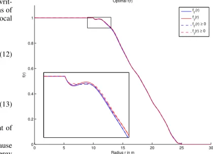
Finally, the code for all the numerical experiments will be freely available on the authors website to promote reproducible research2. 2 http://remi.flamary.com/soft.html 0 5 10 15 20 25 30 0 0.2 0.4 0.6 0.8 1 Radius r in m f(r) Optimal f(r) f Γ(r) f γ(r) f Γ(r) ≥ 0 f γ(r) ≥ 0
Fig. 3. Radial cut of the attenuation of the functions f (r) for aperture and focal optimization at a wavelength of 562 nm. The dashed curves denoted as ≥ 0 correspond to an optimization with α ≥ 0 constraint.
4.2. Optimization for monochromatic light
For a single monochromatic wave, here λ = 562 nm, we have represented the apodizing curves fΓ(r) and fγ(r) in Fig. 3 and
the resulting intensities ΨΓ(r) and Ψγ(r) (top curves), and ΦΓ(θ)
and Φγ(θ) (bottom curves) in Fig.4. We emphasize that these
curves were obtained assuming a perfect circular telescope of radius R. The f -curves are only slightly different and are really similar to a linear apodization. Moreover, in the monochromatic case, enforcing a monotonic f leads to the same results for the thickness of the trace, which will not be the case anymore for a wide spectral bandwidth, as we show below.
The results for the Ψ and Φ-curves are quite different. The residual starlight ΨΓ(r) is very well attenuated across the
tele-scope pupil, as found by Vanderbei et al. (2007). In contrast, Ψγ(r) presents a center-to-limb decrease which suggests an
apodized structure. It is interesting to note the behavior of the curves beyond the region of optimization. There, the relative po-sition of the curves is reversed very rapidly, the focal plane opti-mization becoming lower than the pupil plane optiopti-mization. This is an aspect that deserves further studies.
The intensity in the focal plane is also very interesting. While fΓtends to minimize the intensity at all angles θ, fγonly focuses
on the region of interest, and a strong residual light is observed in the blind area behind the occulter.
The resulting flux Γ, γ for all the different optimizations is given in the upper part of Table 1. Interestingly, fΓ leads to a
flux Γ in the aperture plane 105times fainter than f
γ.
Neverthe-less, in the focal plane the flux γ in the observation area is ≈ 50 times fainter when using fγ. This clearly shows the importance
of using focal plane optimization for optimal apodization.
4.3. Optimization for a wide spectral bandwidth
Next we investigated the two optimization strategies on a wide bandwidth. For this we compute a regular sampling in the in-terval λ ∈ (380,750) nm and computing the average flux across λ. Note that both a sampling of 20 and 100 values were investi-gated, and while we used in the experiments a sampling of 100 for a better precision, the final results were very similar. In
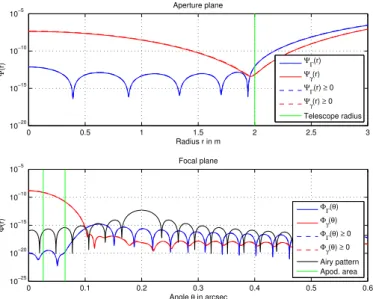
prac-0 0.5 1 1.5 2 2.5 3 10−20 10−15 10−10 10−5 Radius r in m Ψ (r) Aperture plane Ψ Γ(r) Ψ γ(r) Ψ Γ(r) ≥ 0 Ψ γ(r) ≥ 0 Telescope radius 0 0.1 0.2 0.3 0.4 0.5 0.6 10−25 10−20 10−15 10−10 10−5 Angle θ in arcsec Φ (r) Focal plane ΦΓ(θ) Φ γ(θ) ΦΓ(θ) ≥ 0 Φ γ(θ) ≥ 0 Airy pattern Apod. area
Fig. 4. Top curves: intensity in the telescope aperture plane for an opti-mization that minimizes the integrated intensity Γ in the aperture plane (blue curve) or γ for optimizing the observation between 0.1 and 0.5 arc-sec in the focal plane (red curve), for λ = 562 nm. Note the apodization profile for the γ curve and the inversion of relative position of the curves outside the region of optimization. Bottom curves: focal plane intensity obtained for the two optimizations. An airy pattern corresponding to a
10−12fainter exoplanet in the observation area is reported in black. The
apodization area defined by the smallest and largest radius of the occul-ter is also reported in green. Note the inversion of behavior of curves with regard to the overall occulter profile.
tice the variation of the wavefront is extremely smooth w.r.t. λ and the selected sampling in sufficient.
For multiple wavelengths, λ ∈ (380,750) nm, the results are very different. First the optimal functions are much more similar, as illustrated in Figure 5. The functions also tend to oscillate and the monotonic variants are this time different from the free variant of the optimal functions.
The resulting intensities in the aperture and focal plan are plotted in Figure 6. In the aperture plane, the intensity is still apodized for fΓ, but the flux is much more attenuated than in the
monochromatic case. In the focal plane, the intensities retain the same tendencies, but the gain due to the focal plane optimization is lower. Interestingly, enforcing a monotonic function through α ≥0 leads to a clear loss in terms of attenuation for both fΓand
fγ.
In terms of quantitative performances, Table 1 (lower part) shows that the flux in the observation area of the focal plane is still more attenuated with fγ with a gain of 1.9 in the chromatic
case (1.6 with positivity constraint). While the gain in perfor-mance is smaller than in the monochromatic case, it is far from negligible when observing faint objects around a star. Interest-ingly, in the chromatic case, the α ≥ 0 constraint leads to a loss of 2 in attenuation (for both fΓand fγ), proving that relaxing the
constraint can lead to additional gain as long as the apodization is physically realizable.
An additional visualization comparing the performances of fΓversus fγ in the focal plane is given in Fig. 7. The intensity
Φγ(θ) is plotted as a function of ΦΓ(θ) for θ ∈ (0, 0.7) arcsec. The
red line allows a comparison between the methods; if a curve is below this line, it means that Φγ(θ) < ΦΓ(θ) and vice versa.
We clearly see that Φγ(θ) > ΦΓ(θ) for θ < θ1 in the blind area
behind the occulter and that Φγ(θ) < ΦΓ(θ) ∀θ ∈ (θ1, θ2) in the
0 5 10 15 20 25 30 0 0.2 0.4 0.6 0.8 1 Radius r in m f(r) Optimal f(r) f Γ(r) f γ(r) f Γ(r) ≥ 0 f γ(r) ≥ 0
Fig. 5. Radial cut of the attenuation of the functions f (r) for aperture and focal optimization for the whole spectral bandwidth between 380 nm and 750 nm. 10−18 10−17 10−16 10−15 10−14 10−13 10−18 10−17 10−16 10−15 10−14 10−13 ← θ=0.1 arcsec ← θ=0.5 arcsec Φ Γ Φγ Trajectory (Φ Γ(θ),Φγ(θ))
Optim. zone in foc. plane Φ
Γ=Φγ
Fig. 7. Parametric plot of the observed intensities in the focal plane: x-axis, aperture plane optimization, y-x-axis, focal plane optimization. The curve is drawn for the wide spectral bandwidth without positivity con-straints. From top-right to bottom-left the curve follows the increase of θ, clearly showing the concentration of light behind the occulter for the focal plane optimization. The line y = x clearly shows that the γ-curves always give better results than the Γ-curves, especially in the observa-tion area (reported in green).
observation area of the focal plane (illustrated in green in the figure).
4.4. Tolerance analysis to positioning errors of the telescope
A study of the tolerance sensitivity to positioning errors for a 4m circular telescope out of its on-axis position was carried out up to an offset of 1 m.
Because of this offset, the resulting pupil plane and focal plane intensities are no longer circularly symmetric, and the computation of the final focal plane image can no longer use the Hankel transformation of Eq.2. The focal plane image must
R. Flamary and C. Aime: Optimization of starshades 0 0.5 1 1.5 2 2.5 3 10−15 10−10 Radius r in m Ψ (r) Aperture plane Ψ Γ(r) Ψ γ(r) Ψ Γ(r) ≥ 0 Ψγ(r) ≥ 0 Telescope radius 0 0.1 0.2 0.3 0.4 0.5 0.6 10−20 10−18 10−16 10−14 10−12 Angle θ in arcsec Φ (r) Focal plane Φ Γ(θ) Φ γ(θ) Φ Γ(θ) ≥ 0 Φ γ(θ) ≥ 0 Airy pattern Apod. area
Fig. 6. Same representation as in Fig. 4, but for an optimization made for the whole spectral bandwidth between 380 nm and 750 nm. The behavior of the inversion of the curves is similar to the monochromatic case, although it is somewhat reduced by the effect of the chromatism.
Table 1. Resulting light flux in the aperture (Γ) of focal plane (γ) for all the optimization schemes. The upper part of the table corresponds to an optimization on a unique wavelength λ, whereas the lower part of the table corresponds to an optimization on a large spectrum.
λ Flux fΓ(r) fΓ(r) ≥ 0 fγ(r) fγ(r) ≥ 0 Flux ratio Flux ratio ≥ 0
λ=562 nm Γγ 9.07e-137.66e-13 9.55e-138.06e-13 5.06e-081.38e-14 5.52e-081.44e-14 1.79e-05 1.73e-05 5.57e+01 5.61e+01 λ ∈(380,750) nm Γγ 2.91e-13 5.88e-13 2.63e-12 7.01e-12 1.11e-01 8.38e-02 7.08e-14 1.42e-13 3.74e-14 8.99e-14 1.89e+00 1.58e+00
be computed taking the modulus squared of the two-dimensional Fourier transform of the complex amplitude of the wave on the telescope aperture.
In practice, the study was made using a discrete Fast Fourier Transform of an array of 1024 × 1024 points corresponding to an overall zone of 20 × 20 meters, inside which the telescope of diameter 2m was defined by 1 or 0 transmitting pixels over about 205 points in diameter. As a result, altogether 33 081 points were set equal to 1. This percentage of zero-padding is enough to ob-tain a satisfactorily sampled focal plane image.
Positioning errors were simulated by moving the complex amplitude obtained in the shadow of the occulter over the tele-scope aperture in one direction, by steps of 1 pixel or about 2 cm. The two-dimensional array was filled using an interpolation of the one-dimensional complex amplitude of the wavefront com-puted with Eq. 1.
The focal plane image was obtained taking the modulus squared of the Fourier transform of the wave on the telescope aperture. The effect of wavelength was taken into account af-terward. The diffraction pattern increases in size with the
wave-length. For that, a two-dimensional interpolation of the result was used to resample the image. Moreover, a scaling factor in intensity inversely proportional to the square of the wavelength was applied, as in Eq.4. As a result, the integrated flux in the focal plane becomes wavelength independent and equal to that crossing through the telescope aperture. As before, for the sake of simplicity, we assumed that the received flux is constant over the spectral bandwidth.
Figures 8 and 9 present results obtained for transverse dis-placements of the telescope up to 1 m from its nominal posi-tion. We recall that the occulter shapes optimize the measure-ment when the telescope is at its nominal on-axis position, ei-ther for the integrated intensity on the telescope aperture, or for a region in the focal plane between 0.1 and 0.5 arcsec. In both cases the computation was made for the whole bandwidth of λ ∈ (380,750) nm.
Three-dimensional representations of the normalized inten-sities in the telescope aperture were used to enhance differences of intensities in the results of the two optimizations, and the apodization-like pattern obtained for the focal plane
optimiza-Fig. 8. Top curves: pupil plane intensities for an offset of 1 m for λ ∈ (380,750) nm. Density curves below represent the focal plane intensities (log scale) for telescope positions: on-axis (upper curves) and offsets of 50 cm (intermediate curves) and 1 m (lower curves). Left: aperture optimization, right: focal plane optimization.
tion. Both curves were clipped to make the central parts of the images well visible. As expected, there is much less light for the aperture plane minimization when the telescope is at its nominal position. Since the optimization was calculated for a 4m diam-eter telescope, there is a rise in the intensity at the edges for this large offset. This increases becomes somewhat surprisingly in favors of the focal plane optimization for a large off-set, as already discussed in Fig. 6.
In Fig. 8 focal plane intensities are also represented in color levels, with a common color scale for the telescope on-axis and off-axis of 50 cm and 1m. The two circles of radius θ1 = 0.1
arcsec and θ2 = 0.5 arcsec define the angular area inside which
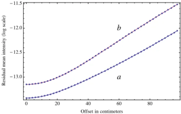
the residual intensity is integrated. The focal plane optimization is found to always be better than the aperture plane optimiza-tion. From comparing these curves, it is clear that the residual diffracted light remains concentrated longer inside the first cir-cle for the focal plane optimization, which is especially cir-clear for the 50 cm offset images. This behavior is confirmed by Fig. 9 which represents the integrated intensity in this region with a logarithmic scale. 0 20 40 60 80 -13.0 -12.5 -12.0 -11.5 Offset in centimeters Res idual mean intens ity Hlog scale L a b
Fig. 9. Average residual light level γ for the focal plane (a) and pupil plane (b) optimization, as a function of the telescope offset in centime-ters for λ ∈ (380,750) nm. The average is computed over the region from 0.1 to 0.5 arcsec delimited in Fig. 8 by two circles.
5. Conclusion
We addressed the problem of optimizing of the shape of a cir-cularly symmetric apodized occulter. To this end, we proposed a general expression for the attenuation function, as a weighted sum of basis functions. We expressed the optimization problem as the minimization of the flux, first in the pupil plane, as is com-monly done in the literature, and then in the focal plane of a 4.m diameter telescope, for a region between 0.1 to 0.5 arcsec in which the exoplanet is supposed to be observed.
Numerical experiments show that the focal plane optimiza-tion leads to a better attenuaoptimiza-tion of the starlight than the pupil plane optimization. One interesting result is that while the focal plane optimization leads to a strong flux in the pupil plane, most of this light is concentrated in the area behind the occulter in the focal plane, which is not a problem for a perfect telescope. Finally, the robustness of our approach to lateral misalignment of the occulter was investigated and showed that the focal plane optimization also yields a better robustness.
As already indicated, the optimization study was made for a 4m telescope assumed to be at its on-axis position. A simple procedure to make the experience less sensitive to defect posi-tion would be to perform the optimizaposi-tion for a larger aperture than is actually used. A better procedure would be to estimate the statistics of pointing errors and include them in the optimiza-tion procedure. Then a better tolerance to pointing errors would be obtained, probably at the expenses of a tolerable loss in the starlight rejection. Nevertheless, our analysis showed that tele-scope offsets of a few decimeters will not strongly reduce the efficiency of the occulter.
This conclusion was obtained for the condition that the tele-scope has a perfectly circular aperture and another study is re-quired to model a telescope with central obscuration. Moreover, it would be interesting to study the effect of a a more realistic telescope with small defaults of phase and amplitude. Deviations from this perfection could lead to somewhat different results, but the exigency of quality is limited to a maximum of 0.5 arcsec, or about twenty Airy rings for a 4m diameter telescope. Finally, with the knowledge of the exact PSF of the telescope, one can readily adapt our optimization approach. A comparison of pupil vs focal optimization for the maximum-magnitude minimization as in Kasdin et al. (2013) would also be interesting.
R. Flamary and C. Aime: Optimization of starshades
Appendix A: Quality test of the numerical
computation using an analytical expression for a sharp-edged circular occulter
Aime (2013) has shown, using an approach similar to Born & Wolf (1999), that an analytic expression using Lommel series could be derived for the Fresnel diffraction of a sharp circular occulter of the form f (r) = f•(r, Ω) = Π(r/Ω), defining here
Π(r) as the function equal to 1 for |r| ≤ 1 and 0 otherwise. At the wavelength λ, the complex amplitude ψ•(r, Ω) of the wave at the
distance z for
(i) inside the geometrical umbra (r < Ω) and (ii) outside (r > Ω),
can be written using two series: ψ•(r, Ω) = (i) τ(r) τ(Ω) ∞ X n=0 (−i)n(r Ω) nJ n(2πΩr λz ) (ii) 1 − τ(r) τ(Ω) ∞ X n=1 (−i)n(Ω r) nJ n(2πΩr λz ). (A.1)
At r = Ω, both series converge to the same value given by ψ•(Ω, Ω) = 1 2(1 + exp(i 2πΩ2 λz )J0( 2πΩ2 λz )). (A.2)
These series are alternative series for the real and imaginary terms, and according to the Leibniz estimate, an upper bound of the error for the sum limited to n = N terms is given by the absolute value of the N + 1 term. The convergence is easy when r/Ω is smaller than 1, for the first sum for r < Ω inside the ge-ometrical umbra, or the inverse outside. The main error occurs near the transition zone r = Ω.
In Fig.A.1 we compare the analytical and numerical results for an example of a circular occulter of 50 m diameter set at 80 000 km, and for a wavelength of 550 nm. The Lommel se-ries were computed for 100 terms, and there is no difference be-tween the two methods. Results were drawn for the real, imagi-nary, modulus, and unwrapped phase of the Fresnel diffraction. Note that this is just an example, in particular, the real and imag-inary part of the diffraction pattern are highly sensitive to a small variation of any of the parameters. The modulus of the intensity pattern clearly shows the visible Poisson spot at the center of the pattern. The unwrapped phase presents a strong phase variation in the center of the umbra and a quieter structure outside the ge-ometric umbra, that is for a region utilized by the telescope for the planet observation. The consistency between the two analytic and numerical results is recognized here as a proof of the quality of the numerical calculation.
Appendix B: Numerical calculation of linearly apodized basis functions
f
k(r)
As indicated in the body of the paper, we tried several forms for the set of apodized basis functions fk(r), and decided to use
the simple trapezoidal functions described in the body of the pa-per because they affect the final solution the least. We did not succeed in deriving an analytic form for the Fresnel diffraction of these functions, but comforted by the results obtained on the Fresnel diffraction of Π(r/Ω), we used the direct numerical cal-culation of Mathematica.
We recall that these functions are linearly apodized disks of radii varying from 10 m to 25 m in steps of 5 cm, the apodization
0 10 20 30 40 -0.2 0.0 0.2 0.4 0.6 0.8 1.0 1.2
Radial distance in meter
Real par t of Ψ Hr L 0 10 20 30 40 -0.2 0.0 0.2 0.4 0.6
Radial distance in meter
Imaginar y par t of Ψ Hr L 0 10 20 30 40 -3.5 -3.0 -2.5 -2.0 -1.5 -1.0 -0.5 0.0
Radial distance in meter
log scale Ψ Hr L 2 0 10 20 30 40 0 1 2 3 4 5 6 7
Radial distance in meter
U nw rapped phas e of Ψ Hr L in units of 2 Π
Fig. A.1. From top to bottom: real, imaginary, squared modulus and unwrapped phase of ψ(r) for a circular occulter of radius Ω = 25 m (the vertical line) at z = 80000 km for λ = 0.55µ m. The continuous line represents the Lommel series, dots are the result of a direct numerical computation of Eq. 1 using NIntegrate of Mathematica
applies for 5 cm at the edge. The resulting ψk(r) are very similar
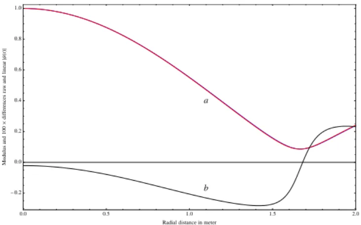
to those obtained for the functions Π(r/Ω). Differences between moduli are lower than 1%, as shown in Fig. B.1 for two extreme cases, but essential to obtain proper results on diffraction pat-terns. In Fig. B.2 we focus on the central part of the diffraction pattern, for r ≤ 2 m. Curves are drawn for a raw and linearly apodized occulter of 10 m and 10.05 m.
0 10 20 30 40 -0.006 -0.004 -0.002 0.000 0.002 0.004 0.006
Radial distance in meter
lin scale dif fer ence Ψk Hr L - Ψ0 Hr L
Fig. B.1. Differences of moduli of Fresnel diffractions for raw and lin-early apodized functions for Ω values of 10 m (thick curve) and 10 m (thin curve). 0.0 0.5 1.0 1.5 2.0 -0.2 0.0 0.2 0.4 0.6 0.8 1.0
Radial distance in meter
M odulus and 100 ´ dif fer ences raw and linear Ψ Hr L a b
Fig. B.2. Representation for r between 0 and 2 m of the moduli of ψk(r)
of linearly apodized occulters of radii 10 m and 10.05 m (a). The two curves are almost over imposed, and curve (b) represents 100 times their differences.
Acknowledgements. We want to thank the referee Jeremy Kasdin for his very constructive comments, and in particular for his suggestion to study the effect of telescope misalignment. This work was granted access to the HPC and visualiza-tion resources of Centre de Calcul Interactif hosted by Université Nice Sophia Antipolis(http://calculs.unice.fr/en).
References
Aime, C. 2013, A&A, 558, A138
Arenberg, J. W., Lo, A. S., Glassman, T. M., & Cash, W. 2007, Comptes Rendus Physique, 8, 438
Born, M. & Wolf, E. 1999, Principles of optics: electromagnetic theory of prop-agation, interference and diffraction of light (CUP Archive)
Boyd, S. & Vandenberghe, L. 2004, Convex optimization (Cambridge university press)
Brueckner, G. E., Howard, R. A., Koomen, M. J., et al. 1995, Sol. Phys., 162, 357
Cash, W. 2006, Nature, 442, 51 Cash, W. 2011, ApJ, 738, 76
Copi, C. J. & Starkman, G. D. 2000, ApJ, 532, 581
Evans, J. W. 1948, Journal of the Optical Society of America (1917-1983), 38, 1083
Jacquinot, P. & Roizen-Dossier, B. 1964, Progress in Optics, 3, 29
Kasdin, N. J., Vanderbei, R. J., Sirbu, D., et al. 2013, in Proceedings of the 2013 IEEE Aerospace Conference
Koutchmy, S. 1988, Space Sci. Rev., 47, 95
Lemoine, D. 1994, The Journal of chemical physics, 101, 3936 Lyot, B. 1939, MNRAS, 99, 580
Marchal, C. 1985, Acta Astronautica, 12, 195 Mayor, M. & Queloz, D. 1995, Nature, 378, 355
Newkirk Jr, G. & Bohlin, J. 1965, in Annales d’Astrophysique, Vol. 28, 234
Purcell, J. & Koomen, M. 1962, J. Opt. Soc. Am, 52, 596 Shiri, S. & Wasylkiwskyj, W. 2013, Journal of Optics, 15, 035705
Soummer, R., Valenti, J., Brown, R. A., et al. 2010, in Society of Photo-Optical Instrumentation Engineers (SPIE) Conference Series, Vol. 7731, Society of Photo-Optical Instrumentation Engineers (SPIE) Conference Series Spitzer, L. 1962, American Scientist, 50, 473
Vanderbei, R. J., Cady, E., & Kasdin, N. J. 2007, ApJ, 665, 794
Vanderbei, R. J. & Shanno, D. F. 1999, Computational Optimization and Appli-cations, 13, 231
Vives, S., Lamy, P., Koutchmy, S., & Arnaud, J. 2009, Advances in Space Re-search, 43, 1007
Wasylkiwskyj, W. & Shiri, S. 2011, Journal of the Optical Society of America A, 28, 1668