HAL Id: hal-00848876
https://hal.inria.fr/hal-00848876
Submitted on 29 Jul 2013
HAL is a multi-disciplinary open access
archive for the deposit and dissemination of
sci-entific research documents, whether they are
pub-lished or not. The documents may come from
teaching and research institutions in France or
abroad, or from public or private research centers.
L’archive ouverte pluridisciplinaire HAL, est
destinée au dépôt et à la diffusion de documents
scientifiques de niveau recherche, publiés ou non,
émanant des établissements d’enseignement et de
recherche français ou étrangers, des laboratoires
publics ou privés.
Non-Coplanar microphone Arrays
Xavier Alameda-Pineda, Radu Horaud, Bernard Mourrain
To cite this version:
Xavier Alameda-Pineda, Radu Horaud, Bernard Mourrain. The Geometry of Sound-Source
Localiza-tion using Non-Coplanar microphone Arrays. WASPAA 2013 - IEEE Workshop on ApplicaLocaliza-tions of
Signal Processing to Audio and Acoustics, Oct 2013, New Paltz, United States. pp.1-4,
�10.1109/WAS-PAA.2013.6701896�. �hal-00848876�
THE GEOMETRY OF SOUND-SOURCE LOCALIZATION
USING NON-COPLANAR MICROPHONE ARRAYS
Xavier Alameda-Pineda
1,2, Radu Horaud
1and Bernard Mourrain
3 1INRIA Grenoble Rhˆone-Alpes,
2Universit´e de Grenoble,
3INRIA Sophia Antipolis, France
ABSTRACT
This paper addresses the task of sound-source localization from time delay estimates using arbitrarily shaped non-coplanar micro-phone arrays. We fully exploit the direct path propagation model and our contribution is threefold: we provide a necessary and suf-ficient condition for a set of time delays to correspond to a sound source position, a proof of the uniqueness of this position, and a localization mapping to retrieve it. The time delay estimation task is casted into a non-linear multivariate optimization problem con-strained by necessary and sufficient conditions on time delays. Two global optimization techniques to estimate time delays and local-ize the sound source are investigated. We report an extensive set of experiments and comparisons with state-of-the-art methods on simulated and real data in the presence of noise and reverberations. Index Terms— Sound source localization, time delay estimate, constrained multivariate non-linear optimization.
1. INTRODUCTION
Source localization from time delay estimates (TDEs) has proven to be an extremely useful methodology with a variety of appli-cations in such diverse fields as aeronautics, telecommuniappli-cations and robotics. We focus on general-purpose TDE-based models for sound-source localization in indoor environments. This is ex-tremely challenging because: (i) there may be several sound sources over time, (ii) regular rooms are echoic (leading to reverberations), and (iii) the microphones are often embedded (robot heads, smart phones, etc.), thus generating high noise.
The TDE problem has been very well investigated and a re-view can be found in [1]. The vast majority of existing approaches deal with one microphone pair, but it is not straightforward to ex-tend most of these methods to more than two microphones. Meth-ods addressing multichannel TDE can be roughly divided into two categories: methods estimating the acoustic impulse responses and methods exploiting the redundancy among several microphones. [2] is illustrative of the first category where a method based on gen-eralized eigenvalue decomposition is proposed. The second cate-gory is represented by [3] where a multichannel criterion based on cross-correlation is introduced to estimate time delays using a linear microphone array. A method using the geometric constraints from multiple microphone arrays is proposed in [4]. In [5], a multi-source counting and localizing algorithm is introduced using uniform cir-cular arrays. In [6], the authors proposed a method for joint time delay estimation and source localization working on non-coplanar microphone arrays. Unfortunately, since it is based on local mini-mization, this method needs to be initialized on a huge grid to find
the global minimum, thus increasing the computational complexity. In most of the cases, experiments are performed on speech data in a
simulatedindoor environment.
This paper has several contributions. We develop a geometric model for sound source localization from TDEs and non-coplanar microphones arrays (Section 3). This model enables the
character-ization of the feasible time delays(those corresponding to an actual source position), the uniqueness of the source position and the
lo-calization mapping, used to retrieve the source position in practice. Since the problem is cast into a non-linear constrained optimization problem, two optimizers are proposed (Section 4). The proposed approach is evaluated on simulated data (as is often the case in the multichannel TDE literature) as well as on real data (Section 5).
2. SIGNAL AND PROPAGATION MODELS We consider a sound source placed at an unknown position S∈ R3. The emitted signal,x(t), is received at M microphones, located at M = {Mm}Mm=1 ⊂ R3. The signal received at themth micro-phone isxm(t) = x(t − tm) + nm(t), where nm, the noise of the mth
microphone, is a zero-mean Gaussian random process, andtm is the time-of-arrival. Assuming direct-path sound propagation at constant speedν, we have tm = kS − Mmk/ν. The time delay between microphonesm and n is:
tm,n(S) = tn− tm=
kS − Mnk − kS − Mmk
ν . (1)
3. PROBLEM GEOMETRY
We recall that the task is to estimate the time delays to further lo-calize the sound source. In this section, we provide the three main theoretical results: (i) the conditions under which a set of time
de-lays correspond to a sound source(such sets will be called feasible sets) and (ii) the uniqueness of the sound source position for any feasible set and (iii) a closed-formula for localization, i.e., to re-trieve the position of the sound source from a feasible set. Even if, in practice the problem is set in the ambient space, R3, the theory presented here is valid in RN,N ≥ 2. In the following, Section 3.1 studies the case of two microphones and Section 3.2 exploits the geometry of theM microphone case.
3.1. The Case of Two Microphones
We start by formally characterizing the set of possible sound-source locations in the case of two microphones located at Mmand Mn.
1
2341
2562
72
89
8A7B
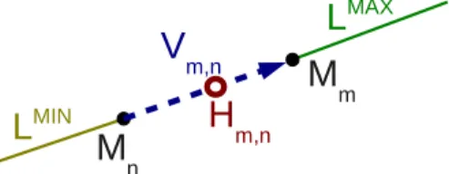
8A7Figure 1: Geometry associated with the two microphone case, lo-cated at Mmand Mn(see Lemma 1). Hm,nis the mid-point of the the microphones (in red) andVm,nthe vector Mm− Mn(in dashed-blue).LMAX
m,n andLMINm,nare the two half lines represented in green and yellow respectively.
For a given time delay ˆtm,n, we characterize S satisfying ˆtm,n = tm,n(S). Because (1) is a hyperboloid in RN, this equation embeds the hyperbolic geometry of the problem. For completeness, we state the following lemma (figure 1):
Lemma 1 The set of sound-source locations S ∈ RN satisfying tm,n(S) = ˆtm,nis: (i). empty if|ˆtm,n| > t ∗ m,n, wheret ∗ m,n= kMm− Mnk/ν,
(ii). the half line LMAXm,n(or LMINm,n), if ˆtm,n= t ∗
m,n(or if ˆtm,n= −t∗
m,n), where LMAXm,n = {Hm,n + µVm,n}, LMINm,n = {Hm,n− µVm,n}, µ ≥ 1/2, Hm,n = (Mm+ Mn)/2
and Vm,n= Mm− Mn,
(iii). the hyperplane passing by Hm,nperpendicular to Vm,n, if ˆ
tm,n= 0 or
(iv). one sheet of a two-sheet hyperboloid with foci Mmand Mn
for other values of ˆtm,n.
Lemma 11and characterizes the positions associated to one micro-phone pair and sets the basis for next section, where we analyze the geometry of the most general microphone setup.
3.2. The Case ofM Microphones in General Position
In this section we characterize the set of possible sound-source lo-cations in the case ofM microphones. We first notice that if a set of time delays ˆt= {ˆtm,n}m=M,n=Mm=1,n=1 ∈ RM
2
satisfies (1)∀m, n, then the time delays are coupled by ˆtm,n = −ˆt1,m+ ˆt1,n. Hence, we only need to consider the time delays t= (t1,2, . . . , t1,M) which lie in a(M − 1)-dimensional vector subspace W ⊂ RM2
. Hence, there areM − 1 equations of the form (1). Geomet-rically, this is equivalent to seek the intersection ofM − 1 hyper-boloids in RN (see figure 2). Algebraically, this is equivalent to solve a system onM − 1 non-linear equations in N unknowns. In general, this leads to search for the roots of a high-degree poly-nomial. However, in our case the hyperboloids share one focus, namely M1. As it will be shown below, the problem in this case reduces to solving a second-degree polynomial plus a linear system of equations. TheM − 1 equations write:
8 > < > : νˆt1,2 = kS − M2k − kS − M1k .. . νˆt1,M = kS − MMk − kS − M1k . (2)
1Proven here: http://hal.inria.fr/docs/00/84/88/39/ PDF/Alameda-WASPAA-2013-Annex.pdf
Figure 2: Localization of the source using four microphones. Their position is shown in black (M1), blue (M2), red (M3) and green (M4). The sound source is placed in the white marker. The blue hyperboloid corresponds to ˆt1,2, the red to ˆt1,3 and the green to ˆ
t1,4. The intersection of the hyperboloids corresponds to the sound source position.
Because theM microphones are in general position (they do not lie in the same hyperplane), we haveM ≥ N + 1, hence the num-ber of equations is greater or equal than the numnum-ber of unkowns. We now provide the conditions on ˆt under which (2) yields a real and unique solution for S. More precisely, firstly we provide a nec-essary condition on ˆt for (2) to have real solutions, secondly we prove the uniqueness of the solution and build a mapping to recover the solution S, and thirdly we provide a necessary and sufficient condition on ˆt for (2) to have a real and unique solution.
Notice that each equation in (2) is equivalent to (νˆt1,m + kS − M1k)2 = kS − Mmk2, from which we obtain −2(M1− Mm)TS+ p1,mkS − M1k + q1,m= 0, where p1,m = 2νˆt1,m andq1,m= ν2(ˆt1,m)2+ kM1k2− kMmk2. Hence, (2) can now be written in matrix form:
MS+ P kS − M1k + Q = 0, (3) where M ∈ R(M −1)×N is a matrix with itsmthrow,1 ≤ m ≤ M − 1, equal to (Mm+1− M1)T, P = (p1,2, . . . , p1,M)Tand Q= (q1,2, . . . , q1,M)T. Notice that P and Q depend on ˆt.
Without loss of generality and because the points M1, . . . , MM do not lie in the same hyperplane, we assume that M can be written as a concatenation of an invertible matrix ML ∈ RN ×N and a matrix ME ∈ R(M −N −1)×N such that M= „ ML ME « . Similarly P = „ PL PE « and Q= „ QL QE « . Thus, (3) rewrites: MLS+ PLkS − M1k + QL = 0, (4) MES+ PEkS − M1k + QE = 0, (5) where PL, QL are vectors in R
N
and PE, QE are vectors in RM −N −1. Notice that (2) is strictly equivalent to (4)-(5). In the following, (4) will be used for defining the necessary conditions on ˆt as well as localizing the sound source. The study of (5) is reported further on. By introducing a scalar variablew, (4) can be written as:
MLS+ wPL+ QL = 0, (6) kS − M1k2− w2 = 0. (7) We remark that the system (6)-(7) is defined in the(S, w) space. Notice that (6) represents a straight line and (7) represents quadric.
Hence the solution to (6)-(7) is the intersection of a straight line and a quadric. In such systems there are two possible configurations: (i) the quadric contains the straight line, and there are an infinite number of solutions, or (ii) the straight line crosses the quadric, and there are two (maybe complex) solutions. In fact, the first case, (i), does not occur. Notice that the quadric is a two-sheet hyperboloid. Because two-sheet hyperboloids are not ruled surfaces, (7) does not contain any straight line. Consequently the system has two (maybe complex) solutions.
In order to solve (6)-(7), we first rerwite (6) as
S= Aw + B, (8)
where A= −M−1
L PLand B= −M −1
L QL, and then substitute S from (8) into (7) obtaining:
(kAk2− 1)w2+ 2 hA, B − M1i w + kB − M1k2 = 0. (9) We are interested in the real solutions, that is, S ∈ RN. Because A, B ∈ RN
, the solutions of (6)-(7) are real, if and only if, the solutions to (9) are real too. Equivalently, the discriminant of (9) has to be non-negative. Hence the solutions to (6)-(7) are real if and only if ˆt satisfies:
∆(ˆt) = hA, B − M1i2− kB − M1k2(kAk2− 1) ≥ 0. (10) The previous equation is a necessary condition for (6)-(7) to have real solutions. Albeit, we are interested in the solutions of (4). Ob-viously, if S is a solution of (4), then(S, kS − M1k) is a solution of (6)-(7). However, the reciprocal is not true; these two systems are not equivalent. Indeed, since∆(ˆt) = ∆(−ˆt), one of the solutions of (6)-(7) is the solution of (4) and the other is the solution of (4) replacing ˆt by−ˆt. In other words, the two solutions of (6)-(7), namely(S+, w+) and (S− , w− ), satisfy either: t(S+) = ˆt t(S− ) = −ˆt or t(S+) = −ˆt t(S− ) = ˆt
Consequently, the solution to (4) is unique. Moreover, we can use (8) to define the following localization mapping, which retrieves the sound-source position from a feasible ˆt:
L(ˆt) = S+= Aw++ B if t(S+) = ˆt S− = Aw− + B otherwise. (11) Until now we provided the condition for equation (4) to have real solutions, the uniqueness of the solution and a localization mapping. However, the original system includes also equation (5). In fact, (5) addsM −N −1 constraints onto ˆt. Indeed, if (L(ˆt), kL(ˆt)−M1k) is the solutions to (4), then in order to be a solution of (4)-(5), it has to satisfy:
E(ˆt) = MEL(ˆt) + PEkL(ˆt) − M1k + QE = 0. (12) Moreover, the reciprocal is true. Summarizing, the system (4)-(5) has a unique solutionL(ˆt) if and only if ∆(ˆt) ≥ 0 and E(ˆt) = 0.
The mappings∆, E and L are explicitly constructed solely from the microphone locations M. Hence, these mappings are not only an interesting mathematical finding in its own right, but also useful from a computational perspective. In addition, the mappings ∆ and E can be understood from two points of view. Geometri-cally, they characterize the time delays corresponding to a sound
source. Algebraically,∆ and E represent the feasibility constraint to the time delay estimation problem, i.e., the time delay estimate should satisfy the necessary and sufficient conditions for the exis-tence of S.L has to be understood as the closed-form solution for
localization, allowing to recover S from any feasible ˆt.
4. TIME DELAY ESTIMATION
In the previous section we characterized the feasible values of t (i.e., those corresponding to a sound source position). But, which is the best value for t, among all the feasible ones? We need a criterion to choose the optimal value for t given theM received signals. This operation is called time delay estimation and the re-sult is the time delay estimator. The criterion we have chosen, de-noted by J, was presented in [3] in the framework of linear mi-crophone arrays and extended in [6] to the non-coplanar case. J is the determinant of the matrix of normalized cross-correlation functions. That is,J(t) := det“[ρi,j(t)]i,j
” , whereρi,j(t) = E{xi(t + t1,i)xj(t + t1,j)} / q E{x2 i(t)} E˘x2j(t)¯, E being the expectation. Notice thatJ increases with the dissimilarity of the signals{x1(t), x2(t + t1,2), . . . , xM(t + t1,M)}.
Thus, the time delay estimation is casted into the following
non-linear constrained optimizationproblem: 8 > > < > > : min t J(t), s.t. t∈ W, −t∗ ≤ t ≤ t∗ , ∆ (t) ≥ 0, E (t) = 0, (13) whereW, t∗
,∆ and E were defined in the previous section. In order to solve this optimization problem, we investigate two distinct methods. First, if the functionsρi,jare continuously differ-entiable, the cost functionJ is Lipschitz continuous in the compact set−t∗
≤ t ≤ t∗
, and hence a branch and bound (B&B) global optimization algorithm is appropriate. Its output is a list of points (ranked by the cost), from which we select the best among those satisfying the constraints. Second, we conjecture that the global minimum ofJ corresponds to local maxima of the functions ρ1,m. Thus, for each microphone pair(1, m), we extract K local maxima ofρ1,m. We then construct a grid with all possible combinations of these values, ending up withKM −1points. This point grid (which is sparser than the one used in [6]) is then used to initialize a log-barrier interior point method.
5. EXPERIMENTAL RESULTS
In order to accurately validate the proposed geometric model and the two optimization algorithms, we developed a formal evaluation protocol using simulated and real data. The setup is the same in both cases: a4 × 4 × 4 meter room with an array of four microphones at (in meters) M1 = (2.0, 2.1, 1.83)T, M2 = (1.8, 2.1, 1.83)T, M3 = (1.9, 2.2, 1.97)T and M4 = (1.9, 2.0, 1.97)T and the sound source at 189 different positions on a 1.7 m radius sphere around the microphones. The source emitted speech fragments ran-domly chosen from [7]. One hundred millisecond cuts of these sounds are the input of the evaluated methods. In the simulated case, we control two parameters. First, the SNR, regulating the amount of noise added to the received signals, and taking the following values (in dB):−10, −5 and 0. Secondly the T60, used in the Image-Source Model [8] to control the amount of reverberations, taking the following values (in s):0 (none), 0.2 (moderate), and 0.6 (se-vere). In the real case, we used the acquisition protocol defined in [9], replacing the dummy head by the tetrahedron microphone array. Several algorithms are compared: D is the method proposed in [6] (optimization solved by a log-barrier interior-point method), I solves independently for each microphone pair, B corresponds to
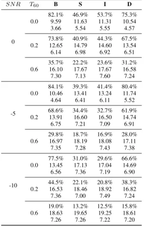
Table 1: Results obtained with simulated data. The first column corresponds to the values ofSN R [dB]. The second column corre-sponds to the values ofT60[s]. The four last columns correspond to each of the methods. For each combinationSN R-T60-method there are three values: the proportion of inliers (angular error< 30 degrees), the inlier angular error mean and standard deviation.
SN R T60 B S I D 0 0.0 82.1% 46.9% 53.7% 75.3% 9.59 11.63 11.31 10.54 3.66 5.54 5.55 4.57 0.2 73.8% 40.9% 44.3% 67.5% 12.65 14.79 14.60 13.54 6.14 6.98 6.92 6.51 0.6 35.7% 22.2% 23.6% 31.2% 16.10 17.67 17.67 16.58 7.30 7.13 7.60 7.24 -5 0.0 84.1% 39.3% 41.4% 80.4% 10.46 13.41 13.24 11.74 4.64 6.41 6.11 5.52 0.2 68.6% 34.4% 32.7% 61.9% 13.91 16.60 16.50 14.74 6.75 7.21 7.09 6.91 0.6 29.8% 18.7% 16.9% 28.0% 16.97 18.19 18.08 17.11 7.35 7.28 7.43 7.38 -10 0.0 77.5% 31.0% 29.6% 66.6% 13.45 17.13 17.04 14.69 6.56 7.36 7.19 6.90 0.2 44.5% 22.1% 20.8% 38.3% 16.53 18.46 18.92 16.82 7.36 7.00 7.49 7.24 0.6 19.0% 13.2% 12.5% 15.8% 18.63 19.65 19.25 18.61 7.26 7.26 7.22 7.20
the B&B method, and S corresponds to the log-barrier interior point methods initialized with the grid proposed in Section 4. All these algorithms provide a time delay estimate, ˆt, used to retrieve the sound-source position using the localization mapping (11).
Table 1 shows the localization results obtained with simulated data. Each row consists on three subrows: the percentage of lo-calization inliers (angular error less than300), the angular error mean of inliers, and the standard deviation (in degrees). We first observe that all methods behave as expected with increasing levels of noise and reverberations. Secondly, we notice that methods B and D perform much better than S and I. Also, we remark that the global optimization procedure proposed in this paper (B) performs systematically better than the state-of-the-art method reported in [6] (D).
Table 2 presents the results on the real data. First of all, we ob-serve that methods D and B outperform S and I as in the simulated case. Secondly, we remark that, contrary to the simulated data, D outperforms B. Third, we notice that the results on real data roughly correspond to the simulated case withT60= 0.6 s and SN R = −5 dB, which is a very challenging scenario. A general remark is that, in all cases the performance notably decreases with reverberations, which is expected, since the signal model used does not explicitly handle the reverberations.
Table 2: Results obtained with real data. The rows have the same meaning as in Table 1.
B S I D
21.98% 12.77% 13.14% 27.64% 18.15 19.01 18.79 16.16
7.17 6.83 7.06 7.58
6. CONCLUSIONS AND FUTURE WORK
In this paper we derived a geometric model for arbitrary shaped non-coplanar microphone arrays, providing a characterization of the feasible time delays and a localization mapping to recover the sound source position. The task is casted into a non-linear optimization problem constrained by the geometric model. Two algorithms are proposed to find the optimal solution and localize the sound source. Extensive experiments on both simulated and real data allow us to conclude that the the proposed model in conjunction with the B&B algorithm outperforms the state of the art, thus validating the geo-metric model as well as the optimization procedure.
We will extend this work in several directions. Firstly, learn-ing the effect of the reverberations on the objective function. Sec-ondly, by evaluating the model in the framework of dynamic sound sources. Thirdly, adapting the methodology into a calibration task, where the position of the sound source may be known, but not the microphones’ position. Finally, performing experiments using a large number of microphones and evaluating the influence of their positions.
7. REFERENCES
[1] J. Chen, J. Benesty, and Y. A. Huang, “Time Delay Estimation in Room Acoustic Environments,” EURASIP, 2006.
[2] S. Doclo and M. Moonen, “Robust Adaptive Time Delay Es-timation for Speaker Localization in Noisy and Reverberant Acoustic Environments,” EURASIP, 2003.
[3] J. Chen, J. Benesty, and Y. Huang, “Robust time delay esti-mation exploiting redundancy among multiple microphones,”
IEEE Tran. on SAP, 2003.
[4] A. Canclini, E. Antonacci, A. Sarti, and S. Tubaro, “Acoustic source localization with distributed asynchronous microphone networks,” IEEE Tran. on ASLP, 2013.
[5] D. Pavlidi, A. Griffin, M. Puigt, and A. Mouchtaris, “Real-time multiple sound source localization and counting using a circular microphone array,” IEEE Tran. on ASLP, 2013. [6] X. Alameda-Pineda and R. P. Horaud,
“Geometrically-constrained robust time delay estimation using non-coplanar microphone arrays,” in Proceedings of EUSIPCO, 2012. [7] J. S. Garofolo, L. F. Lamel, W. M. Fisher, J. G. Fiscus, D. S.
Pallett, N. L. Dahlgren, and V. Zue, “Timit acoustic-phonetic continuous speech corpus,” 1993, LDC.
[8] E. A. Lehmann and A. M. Johansson, “Prediction of energy de-cay in room impulse responses simulated with an image-source model,” JASA, 2008.
[9] A. Deleforge and R. P. Horaud, “The cocktail party robot: Sound source separation and localisation with an active bin-aural head,” in IEEE/ACM HRI, 2012.