HAL Id: hal-01880430
https://hal.archives-ouvertes.fr/hal-01880430
Submitted on 24 Sep 2018
HAL is a multi-disciplinary open access
archive for the deposit and dissemination of
sci-entific research documents, whether they are
pub-L’archive ouverte pluridisciplinaire HAL, est
destinée au dépôt et à la diffusion de documents
scientifiques de niveau recherche, publiés ou non,
Leveraging Live Machine Learning and Deep Sleep to
Support a Self-Adaptive Efficient Configuration of
Battery Powered Sensors
Cyril Cecchinel, François Fouquet, Sébastien Mosser, Philippe Collet
To cite this version:
Cyril Cecchinel, François Fouquet, Sébastien Mosser, Philippe Collet. Leveraging Live Machine
Learn-ing and Deep Sleep to Support a Self-Adaptive Efficient Configuration of Battery Powered Sensors.
Future Generation Computer Systems, Elsevier, In press. �hal-01880430�
Leveraging Live Machine Learning and Deep Sleep to
Support a Self-Adaptive Efficient Configuration of
Battery Powered Sensors
Cyril Cecchinel,François Fouquet1
DataThings, Luxembourg
Sébastien Mosser,
Philippe Collet2
Université Côte d'Azur, CNRS, I3S, France
Abstract
Sensor networks empower Internet of Things (IoT) applications by connecting them to physical world measurements. However, the necessary use of limited bandwidth networks and battery-powered devices makes their optimal config-uration challenging. An over-usage of periodic sensors (i.e. too frequent mea-surements) may easily lead to network congestion or battery drain effects, and conversely, a lower usage is likely to cause poor measurement quality. In this paper we propose a middleware that continuously generates and exposes to the sensor network an energy-efficient sensors configuration based on data live obser-vations. Using a live learning process, our contributions dynamically act on two configuration points: (i) sensors sampling frequency, which is optimized based on machine-learning predictability from previous measurements, (ii) network usage optimization according to the frequency of requests from deployed soft-ware applications. As a major outcome, we obtain a self-adaptive platform with an extended sensors battery life while ensuring a proper level of data quality and freshness. Through theoretical and experimental assessments, we demonstrate the capacity of our approach to constantly find a near-optimal tradeoff between sensors and network usage, and measurement quality. In our experimental val-idation, we have successfully scaled up the battery lifetime of a temperature sensor from a monthly to a yearly basis.
1{cyril.cecchinel,francois.fouquet}@datathings.com 2{mosser,collet}@i3s.unice.fr
1. Introduction
The most recent Gartner group’s forecasts predict up to 26 billions of things that could be connected to the Internet by 2020 forming the Internet of Things
(IoT). Once measured, data gathered from IoT sensors are key enablers for next
generation infrastructures such as Smart Cities or Smart Grid.
In sensing infrastructures [1], sensor networks are responsible for measuring physical phenomena and sending values to a remote IoT middleware where the collected data can be retrieved by third-party applications. In addition, such middleware is also responsible for managing the devices deployed in the sensor networks [2]. In particular, the middleware defines how the data is retrieved from the sensor network either using pulling or pushing mechanisms.
Using a pulling approach implies sensors to be always reachable but sensor networks are mainly relying on battery-powered devices and limited bandwidth networks. Due to these constraints, IoT devices are most of the time not directly reachable and need to adopt a push mechanism to share the measured data with a remote middleware. Regardless of the network technology used, the configu-ration of this push mechanism directly impacts resources usage, as well as the chosen measurement frequency. In a nutshell, a sensor loops over a very simple and generic process that consists in measuring, buffering, pushing data, sleep-ing and loopsleep-ing again. Dursleep-ing measursleep-ing, pushsleep-ing and sleepsleep-ing phases, sensors have drastically different battery usages, from milliamp to microamp per hour, as shown by theoretical simulations [3] and empirical validations [4]. In addition, last generation microcontrollers offer much more powerful and easy access deep-sleep modes thanks to the embedded network layers within the chip [5], which can be activated by disconnecting every unnecessary elements such as network chips between two measurements. Usage of deep sleep can shift the battery life of a sensor [6], from days to years! This makes deep sleep the major tool to design energy-efficient protocols [7], relying for instance on sensor network topology [8]. However, under deep sleep, sensors are unreachable and poten-tially can miss important measurements. Therefore, using deep sleep should be subject to a tradeoff between data quality and the battery life as a short deep-sleep allows the sensors to send data more frequently but drains the battery whereas a long deep-sleep saves the battery but prevents the measurement of values.
Moreover, using fixed period data collection is not efficient as, due to lack of foreseen precise data usage, many IoT infrastructures oversample their sensors. This produces sub-efficient datasets and drain devices’ battery. In addition, measured data can be very variable so that a static collection policy will be always sub-efficient. For instance, in a steady state, temperature of a room will be stable and does not require high frequency measurements. Conversely, in heating mode, temperature is less predictable and should be sampled with higher frequency. There are already many machine learning algorithms allowing the construction of predictive models. As an example, considering a public open
dataset of temperature sensors3, more than 90 % of data are redundant as they could have been extrapolated from a prediction model. This advocates for an adaptive strategy [7, 9] that, like cloud computing, adapts resource usage based on observed need [10]. Assuming these data were produced from a battery-powered sensor, it would have over-consumed energy.
We claim that an adaptive strategy could reduce this energy loss, signif-icantly extending the lifetime of the most frequently used batteries in sensor networks. Examples to support this assumption are given in Sec. 3. Imple-menting this vision, we present here a self-adaptive and energy efficient sensor network middleware driven by machine learning. This contribution aims at re-ducing the amount of measured data by sensors in order to reduce the battery consumption of them. To do so, we rely on the predictability property of each sensor signal, calculated by a machine learning algorithm. Overall, our middle-ware relies on learning techniques to compute at any moment the appropriate sampling and pushing period for each connected sensor. These data collection periods are sent to sensors, allowing them to dynamically reconfigure their deep sleep and push periods. To mitigate the risk of missing important measures, deep sleep periods are bounded by a maximum time deviation limit defined by domain experts.
Our contribution also aims at measuring the gain of battery lifetime using such adaptive periods. These experiments were conducted on a prototyping platform running on an ESP8266 architecture powered by a lithium-ion bat-tery. First, we have determined extreme boundaries of microcontroller working conditions by identifying the cutoff voltage (i.e., the minimum voltage at which the platform is still working). Secondly, we have evaluated with fixed sampling periods and adaptive periods the time to reach this cutoff voltage. Then, we have have applied the proposed approach and compare the gain in battery life-time. Experiments were conducted over weeks while accelerating their usage by artificially reducing the sampling period. Nonetheless, extrapolated results show that our adaptive usage of deep-sleep is solely able to extend the battery lifetime from a weekly basis to a one of many months.
In the following, Sec. 2 presents how one can apply live machine learning techniques upon battery-powered sensor to predict futures values. Sec. 3 sup-ports our assumptions by illustrating the need of adaptive periods based on realistic observations. Then, Sec. 4 focuses on the computation of the appro-priate periods while Sec. 5 describes the assessment of the proposed approach on a real platform by observing the battery life-time. Finally, Sec. 7 discusses future work and concludes this article.
3https://github.com/ulrich06/greycat_senso/blob/master/assets/TEMP_CAMPUS_15d.
2. Live machine learning and predictability applied to battery-powered sensors
In this paper we focus on battery-powered sensors for which energy consump-tion is a key criterion to ensure their viability in the long run. To reach their energy efficient goal, such devices are usually designed around a microcontroller architecture such as the widely used ESP8266 [11] manufactured by Espressif Systems. The data-sheet of such hardware highlights the tremendous difference of energy consumption according to the use or the absence of use of elements such as network or measurement devices (e.g., thermo-resistance or wifi chip). In others words, the energy consumption is directly related to the sampling and the sending of measurements. As mentioned in the introduction, a mode called deep-sleep can be activated to drastically reduce energy consumption by stop-ping most of sensor services. As a result the frequency of measurement, network push and deep-sleep activation will have a direct impact on sensor lifespan.
Most of the physical phenomena under measure are inescapably variable. As an example, if a measured temperature is stable, high frequency measurement will waste energy while not participating more to the knowledge acquired about temperature. Based on the variability of physical phenomena and the impact of sampling and sending over the sensor’s battery, this work relies on the following general hypothesis H: “a fixed sampling and sending of measurements
generates redundant data and therefore a waste of energy”.
Live machine learning techniques help to predict data by discovering a model against a dataset and to reduce the energy consumption by reasoning on this model instead of querying new values from the sensors [12]. In the field of statistics, the regression methods, e.g., the linear regression method, allow one to predict one variable from other variables. This type of regression is built from a fixed set of data. If all the data are not known in advance, the regres-sion methods must be updated with the new data. Such updatable methods are known as autoregressive methods. They allow a compact representation of temporal series datasets [13] as they rely on data predictability to recursively try to replace a range of data by a compact model. Usually, the expected out-come is a compression or simplification of data to enhance later processing. For instance, a polynomial function can replace a range of data by its ability to pro-duce within a tolerated error the initial data points. An autoregressive method can then consist at fitting a polynomial function to this range of data.
Our contribution heavily relies on such techniques and data predictability principle, but for another purpose: we use the predictability principle not for
a posteriori compression, but as an input to optimize physical sensor sampling
rate. In other words, we want to use an a priori compression to reduce sensor usage.
In addition, autoregressive methods can be used online, while measurements are streamed from sensors [14]. The benefit is an immediate feedback of the learning method, able to be used immediately. However, this live usage implies a computation cost for every input datum, making the ratio between its efficiency and effectiveness critical.
NOX_SENSOR (sampling= 240min)
sampled value « observed » phenomena « real » phenomena
1h 0 50 100 150 200
max. NOx level
250 300
❶
❷
❶
❶
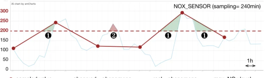
Figure 1: Sampling using a fixed period
To illustrate this tradeoff, we compare a regression method using a lot of buffered data to detect a trend and offer better compression, with an approach without memory which tries to segment data in motion. Due to our live usage with sensors, the performance is key for our approach. For this reason, we rely on polynomial regression model without memory which gives the fastest results according to the tested datasets.
We also note that there are network access protocols designed for battery-powered platforms, but these optimisations are done for mesh networks and are not efficient for client/server architectures promoted by the IoT and IP network everwhere paradigms. We discuss them in section Sec. 6.
3. On the positive influence of automated sampling on power con-sumption
In this section, we discuss how live machine learning techniques can help to predict data and we illustrate the gains of using dynamic sampling and sending periods based on our hypothesis H.
3.1. Impact of automatic sampling period configuration based on sensor pre-dictability
Data obtained from the sensor network are collected according to a collection period. The definition of a fixed collection period leads to important values being missed between two data sampling. For example, Fig. 1 depicts the values
produced by a NOx sensor deployed in an Italian city [15]. The European
Union4expects NO
xhourly average concentrations to be lower than 200µg/m3
or yearly average concentrations to be lower than 40µg/m3. An alert must be
triggered for the inhabitants if these values are exceeded. The sampled values (big dots) obtained from this sensor mislead domain experts. Indeed, with its static collection period, a pollution event is triggered when the pollution is still
4
❶ ❷ ❸ ❶ ❷ ❸ ❶ ❷ ❸ ❶ ❷ ❸
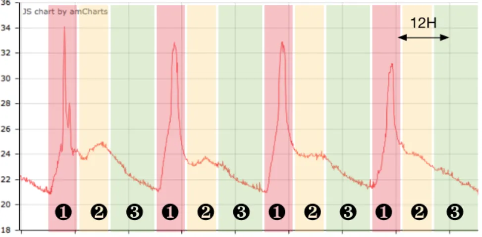
12HFigure 2: Periodic patterns for a temperature sensor
lower than the threshold value or stays active when the pollution episode is over (areas marked with ¶ on Fig. 1), resulting in false alerts. Moreover, some episodes of pollution can be unnoticed (· areas on Fig. 1), which clearly breaks the law.
In addition, a fixed collection period is irrelevant when observed phenomena follow periodic patterns. Fig. 2 presents temperature data collected from a sensor located in an office exposed to direct morning sunlight. The analysis of data using a one-day window highlights a recurrent three-stages pattern: (i) the temperature first rises quickly (sun hitting the windows) before dropping sharply due to the activation of the air conditioning in the morning (¶ on Fig. 2), (ii) then the temperature fluctuates slowly during the day after occupants arrival, as they prefer to switch off the air conditioning and open the window in the afternoon (· on Fig. 2) and (iii) finally, it decreases smoothly over the night (¸ on Fig. 2). As temperature data is varying tremendously during the first stage, a short period of collection is required to reduce the loss. Regarding the second stage, a longer collection period is preferable as values fluctuate slowly. Finally, during the third stage, the collection period can be significantly reduced as values decrease in a linear manner.
In such context, the predictability of physical phenomena can be exploited to increase the data collection period, and thus to lower the energy consumption by reducing the duty cycle and (energy intensive) accesses to the network.
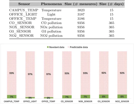
Table Tab. 1 presents several public datasets obtained from real measure-ments. Temperature, light and power consumption values are obtained from
sensors deployed on a campus located in southern France5 [16]. The pollution
Table 1: Datasets from real world experiments (campus [16], pollu-tion [15])
Sensor Phenomena Size (# measures) Size (# days)
CAMPUS_TEMP Temperature 3823 15
OFFICE_LIGHT Light 3187 15
OFFICE_TEMP Temperature 3186 15
CO_SENSOR CO pollution 9356 365
NOX_SENSOR NOx pollution 9356 365
O3_SENSOR O3 pollution 9356 365
NO2_SENSOR NO2 pollution 9356 365
Figure 3: Predictable data from real-environment datasets
values are collected from periodic sensors deployed in an Italian city [15]. The lifetime of batteries powering devices deployed in sensor networks can be extended significantly when sensors are running in a deep-sleep mode. Dur-ing a deep-sleep period, a sensor does not sample or send data over the network. Machine learning algorithms learn from historical data to predict, within a mar-gin of error, a current or future values without requiring any call to the sensor network. In addition to prediction capability, live learning analysis are suitable to reduce the number of values transferred through the network. One of these methods uses polynomial segmentation [17] to represent a phenomenon using a sequence of polynomials functions. In a nutshell, this approach fit a polynomial function while data are received from sensors and append a new polynomial function when a significant change is observed. Polynomial functions are later able to extrapolate any points between the first and last inserted one. The ap-plication of this algorithm on the datasets presented in Tab. 1 shows that more than 90% of the values can be extrapolated from the polynomial functions, cf. Fig. 3, as they fit the previously learn change trend. Considering that these data can be extrapolated, from both sensor and collector server sides, their
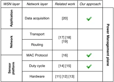
mea-Po w e r Ma n a g e m e n t p la n e Hardware Se n s or p la tfo rm Duty cycle N e tw ork MAC Protocol Routing Transport A p p li c ati o n Data acquisition [11] [12] [13] [14] [15] [16] [17] [18] [19] [20]
WSN layer Network layer Related work Our approach
Figure 4: Cross-layer power management: positioning of your ap-proach
surement and transfer over the network can be saved. For instance, over 15 days,
3823values have been collected from a temperature sensor (CAMPUS_TEMP).
This corresponds to 255 measurements and transfers per day. The application of the polynomial segmentation saves 93% of the values, which shows that only
18 measurements and transfers per day are sufficient to characterize the
phe-nomenon.
3.2. Impact of automatic buffers configuration based on sensor data use fre-quency
Power management is a dominant issue in sensor networks as sensor nodes have a limited amount of energy that determines their lifetime [18]. Energy optimizations are performed at each layer of the protocol stack used by sensing infrastructures (cf. Fig. 4). At the sensor platform stage, power management optimizations mainly target hardware and duty cycle, i.e., the fraction of one period in which the system is active, concerns. At the hardware layer, opti-mizations target mainly battery [19, 20] and platform electronic design [21]. For example, although the platforms ESP-12E and ESP-12 DevKit are built around the same chip, there is a 4.6 ratio between their respective energy con-sumption: 70mA for ESP-12E DevKit and 15mA for ESP-12E in stand-by mode. These consumptions fall respectively to 200µA and 10µA in deep-sleep mode. At the duty-cycle level, optimizations are mostly made by dynamic context-adaptation [22, 23]. With such an adaptation, it becomes possible to set automatically a platform in a deep-sleep mode whenever it is not used for a significant time. At the network level, power management optimizations are
often made in medium access protocols (MAC), routing protocols and trans-port protocols [24]. At the routing and transtrans-port layers, we can observe that many energy efficient protocols have been proposed for WSNs [25, 26, 27]. At the application level, energy optimizations address mainly the data acquisition operations.
These optimizations are tedious to create as applications are outside the WSNs and designed by software engineers that might not have a fully under-standing of the underlying sensing infrastructures. Applications are likely to over-exploit the sensing infrastructure by acquiring data at a tremendous
pe-riod, thus draining batteries to ensure an optimal quality of service. The IETF6
Protocol Suit for the Internet of Things proposes a request/response interac-tion using CoAP [28]. CoAP offers proxy and caching mechanisms allowing last produced values to be acquired without sending requests within the sensor network. Another solution consists in the introduction of a data buffer at the sensor platform layer. Data stored in the buffer are then only sent when needed by applications. Such a method can massively reduce the energy consumption. For instance, according to the ESP 8266 datasheet [11], the microcontroller con-sumption varies between 120 and 170 mA during data transmission which is ten times higher than the power consumption when the network interface is off. 3.3. Towards an adaptive approach for saving energy
In the previous subsections, we have made the following observations :
• (O1)many physical phenomena have a predicable nature [29]. Therefore
we can take advantage of this characteristic to dynamically adjust the
sampling periodof sensors;
• (O2)applications leveraging sensor data could query them at a frequency
lower than the sampling rate needed to capture properly the physical phenomenon. Therefore, we can take advantage of the data usage to adjust the data sending period.
We propose to combine these two observations to opportunistically optimize sampling periods where sensors can configure themselves in deep-sleep mode
(cf. O1) and optimize sending periods to send data only when they are
rele-vant to applications (cf. O2). We expect the combination of these periods to
enhance the battery life-time. Thus, we address the following research question: (RQ) “Can we significantly gain battery lifetime for a whole sensor platform using adaptive sampling and sending periods?”
To tackle this energy optimization problem, we present in the following a tooled approach working at duty cycle, MAC protocol and data acquisition lay-ers, cf. Fig. 4. This tooled approach relies on machine learning techniques that adapt dynamically (i) the sampling period according the predictability of data (Data acquisition and Duty cycle layers) and (ii) the sending period according
the average use by the applications (Data acquisition and MAC protocol layers). Regarding the routing and transport layers, we rely on classical IP routing and UDP protocol.
We conducted an experimental evaluation of the proposed approach on real battery-powered platforms to measure the gain in battery lifetime brought by adaptive periods. For this purpose, the platforms were equipped with a temper-ature sensor and were deployed in a environment where we already had datasets describing the past temperature values. Thus, the computed sampling periods were expected to be related to the temperature variation of the environment. We also mocked several application collective behavior to obtain relevant computed sending periods based on the data usage.
4. Predictive Model
In the previous section, we have discussed how a sensor platform battery is directly impacted by sampling operations, i.e., acquisition of a value, and the network access, i.e., the sending or the retrieval of information through the network. Machine learning techniques can help to predict futures values and thus, reduce the amount of sampling operations. We have also seen that some applications could not require, in a real-time manner, the values measured by sensor platforms. We can also use machine learning to predict when data are necessary and thus, reduce the amount of sending operations.
In this section, we address the adaptive aspect of the research question by introducing a predictive model to compute the appropriate collection periods,
i.e., the appropriate sampling and sending periods.
4.1. Assumptions on the sensing infrastructure
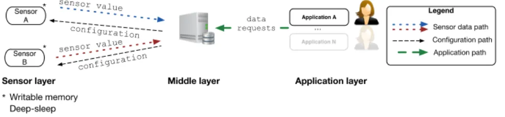
We assume a sensing infrastructure built on three layers (cf. Fig. 5): (i) a sensor network layer containing the sensor platforms that host the sensor and measure environmental phenomena, (ii) a middle layer containing a middleware that stores the sensors values and the sensors configuration, and (iii) an appli-cation layer containing third party appliappli-cations that are fed with sensor values. The sensors send their values to the middleware and retrieve their configuration from this latter.
We also made the following assumptions on the sensor platforms:
• Sensor platforms are powered by batteries and their replacement is a te-dious maintenance operation;
• sensors have a deep-sleep mode allowing them to save energy efficiently when they are not on duty;
• sensors have a writable memory to store their configuration and to buffer their measurements (deep-sleep modes do not guarantee a full retention of RAM) ;
Middle layer configuration configuration sensor value sensor value data requests Legend Sensor data path Application path Configuration path Application A … Writable memory Deep-sleep Battery powered
Sensor layer Application layer
Sensor A * Sensor B * *
Figure 5: Overall sensing infrastructure considered in this paper
• sensors platforms are directly connected to an IP network and can retrieve a new configuration upon demand;
• sensors platforms have limited computation facilities as they are often built on microcontrollers.
4.2. Building a predictive model
We propose to build a predictive model to extrapolate, for a each sensor,
(i) its future values based on its past values and (ii) user’s requests from its
activity history in order to reduce the amount of sampling and sending opera-tions.
However, retaining all sensor past values hardly scales in terms of storage volume. In statistics, linear regression allows one to interpolate (within an acceptable margin of error) a polynomial function from a set of values. Thus, the resulting polynomial function contains in itself the set of values. We leverage this technique on sensor values to store only polynomial functions (describing a set of sensor values) rather than storing raw sensor values. The same observation can be made over activity history. Instead of storing every single sensor’s activity, we compute the overall activity of the sensor, per time-slot.
Given that the computation of these interpolations is resource-intensive, we rely on a middleware located outside the sensor network where servers have higher computing and storage resources suitable for big data analysis. Our
predictive model is built upon the GreyCat7graph database [17] that integrates,
directly into nodes, machine learning algorithms.
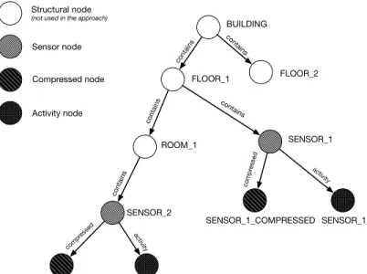
We represent every sensor deployed in the sensor network in a model con-taining a sensor node collecting the received values, a compressed node, i.e., a node performing the autoregression operations, and an activity node, i.e., a node storing the sensor’s activity (cf. Fig. 6).
SENSOR_1_COMPRESSED SENSOR_1_ACTIVITY BUILDING FLOOR_1 FLOOR_2 ROOM_1 SENSOR_1 contains SENSOR_2 SENSOR_2_COMPRESSED SENSOR_2_ACTIVITY contains contains contains contains activity activity compr essed compr essed Sensor node Compressed node Activity node Structural node
(not used in the approach)
Figure 6: Excerpt of a Smart Building representation with activity and compressed nodes for each sensor
Sensor node. A sensor node is responsible for collecting data retrieved from its
associated sensor in the network. This node has a value attribute updated with the latest value coming from the represented sensor. Historical values can be retrieved by reverting the node at a previous time. In the case no value has been stored at the requested time, the node retrieves automatically the freshest previous value.
Compressed node. A compressed node stores sensor data using a polynomial
live segmentation. Polynomial live segmentation is a technique that builds and updates a polynomial function modeling the current trend of data, as shown in Sec. 2. This function is kept as long as it ’fits’ newly measured values, when the contrary happens, an empty polynomial function is created and chained with the previous one.
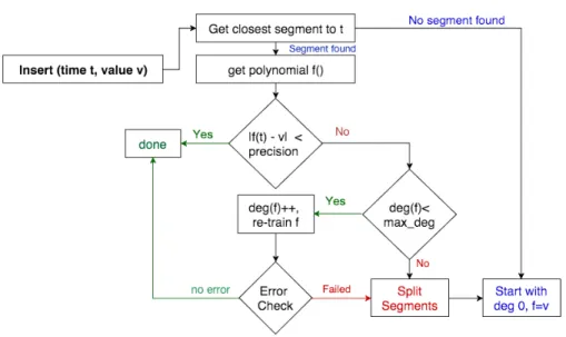
The complete process of live polynomial segmentation is depicted in Figure Fig. 7.
The chaining mechanism works as follows: when a new timestamped t value needs to be inserted, the algorithm gets the closest segment to t. If no segment
is found, a new polynomial fnew (such that deg(fnew) = 0 and fnew = v) is
created. Otherwise, the algorithm checks if the value fits the polynomial f closest segment within a certain precision (chosen by a domain expert). As long as the value fits the closet segment, the polynomial does not need to be updated. Conversely, the algorithm tries to increase f’s degree and re-train f.
Figure 7: Polynomial live segmentation algorithm
In the event f cannot be updated, the algorithm performs a segmentation and
builds a new polynomial fnew.
In other words, whenever data coming from the sensor network is collected, the polynomial live segmentation checks whether it suits the current polyno-mial function or stays within an acceptable margin of error, i.e., no significant change, and then will either increase its degree or leave it unchanged. If the data indicates a significant change, a new polynomial function, continuous to the previous one, will be built.
As a result, the compressed node contains only polynomial functions to rep-resent the data. The ratio between the number of polynomial functions and the number of values stored in the sensor node gives the compression rate.
In [17], the authors of the live polynomial segmentation algorithm gave a mathematical evidence about the ability of this chain of polynomial functions to rebuild the original measured values within a given tolerated error. They also already pinpointed the relation between signal steady state and unchanged polynomial degree after insert. Besides the compression of such segmentation algorithm, this steady state detection is later reused in this paper to compute the optimal sleeping time of sensors.
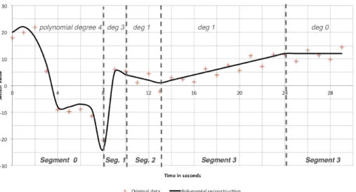
An illustration of this live segmentation algorithm against a simulated signal is shown on Fig. 8. The polynomial reconstruction (black line) interpolates the original data (red crosses) with a certain precision. As long as the original data fits the polynomial or the current polynomial’s degree can be increased, no segmentation is required. Conversely, when the original data’s trend varies greatly (e.g., switching from a variable trend to a steady trend, as shown between
Figure 8: Illustration of the polynomial live segmentation algorithm
Figure 9: Cumulative daily temperature measures accesses (one month)
segments 1 and 2), the algorithm can no longer update the polynomial and builds a new one starting at degree 0 in a new segment.
Activity node. An activity node logs the statistics about data requests using a
gaussian slots representation. These Gaussian slots allow us to predict, given a time slot, the frequency of requests by third-party applications. They are
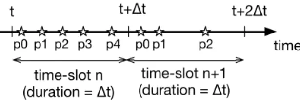
up-time time-slot n (duration = Δt) time-slot n+1 (duration = Δt) p0 p1 p2 p3 p4 p0 p1 p2 t t+Δt t+2Δt
Figure 10: Polynomial functions distribution across time
dated in live, i.e., every time an application requests a data. For instance, the figure Fig. 9 has been obtained from the logging of temperature data accesses during one month and the distribution of these logs in gaussian slots shows that 900 accesses to the temperature produced between 5 pm and 6 pm UTC have been logged in time slot #17. Consequently, these values are highly re-quested and thus the sampling period needs to be shortened to ensure the data availability. Conversely, values produced at night (e.g., 0-6am UTC: time slots #0-6) are never requested by the application and thus, the sending period can be increased to save energy. In the following, we define the activity of a sensor as the number of data accesses during a time slot.
4.3. Optimal data sampling period
As stated previously, it is irrelevant to sample data if the observed phe-nomena can be predicted, e.g., a temperature room remains steady. We thus propose to adapt the sampling period according to the number of significant changes (i.e. the amount of different polynomial functions) in a time-slot. In-deed, a change of polynomial function happens every time the measured value cannot fit further the current prediction. We introduce T the set of time-slots
and ∆t the duration of a time-slot. We also define Pt= {p0, p1, . . . pn} the set
of polynomial functions in a given time-slot t ∈ T and time(p) the time associ-ated to the beginning of a polynomial function (Fig. 10). As it is irrelevant to perform sample operations while the prediction remains valid, we compute, for a time-slot t ∈ T , the time between the beginning of two consecutive polynomial functions, i.e., the amount of time the prediction remains valid:
∆pt= {time(pn+1) − time(pn)}, 0 ≤ n < card(Pt) (1)
If a time-slot t ∈ T contains only one polynomial function p0, we
com-pute the maximum time between time(p0) and the time-slot endpoints, such
as ∆pt = max(∆t − time(p0), time(p0)). In the case the time-slot t ∈ T is
empty and in order to have at least one measurement per time-slot, we define
∆pt = ∆t. These two latter computations can allow the detection of
abnor-mal situations (e.g., a change of temperature because of the sudden heating of a room) in order to integrate these abnormal values into the computation of future polynomial functions. For each time-slot, we compute the minimal time
between two polynomial functions to ensure the best data quality. Thus, we
define the set of minimal sampling periods P sampt∈T as follows:
P sampt= min(∆pt) (2)
Then, the data sampled is stored into a buffer located in a non-volatile
memory (e.g., an EEPROM8) and the platform enables the deep-sleep mode
until the next data sampling or data sending. 4.4. Optimal data sending period
As shown on Fig. 9, data are not always used in real-time or critical appli-cations and therefore, their sending can be deferred to save energy. Thus, we propose to configure the sending period according to the expected use of the data and to buffer the data between two sendings. We reuse the same set of time-slots T and ∆t the duration of a time-slot as introduced before. Given
an activity a(t) produced in time-slot t ∈ T and At∈T the set of all activities
produced in t, we define the set of minimal sending periods P sendt∈T as follows:
P sendt∈T = ∆t/card(At) (3)
The obtained P sendt∈T value corresponds to a fair distribution over time of the
activities. For example, if four activities has been recorded within a time slot and ∆t = 60min, the value P send would be equal to 60/4 = 15min. Thus, the sensor platform would send its buffered values every fifteen minutes.
4.5. Adaptive firmware
Sensor platforms need to retrieve the optimal sampling and sending periods computed on the server-side. To do so, we propose an algorithm that measures data, buffers them and periodically connects to the remote server to send data and retrieve the appropriate sending and sampling periods. The algorithm is depicted in Alg. 1 and can be implemented on platforms with writable memory and connecting facilities, e.g., ESP8266 or RTL8710 based-platforms.
First of all, the sensor platform retrieves the current timestamp (line 1) and the timestamps matching the next sampling and the next data sending (lines 2-3). If the next sampling time is outdated (line 4), the platform performs a measurement that is buffered thereafter. Finally, the platform reads from memory the current sampling period and updates its next sampling time. If the next sending time is outdated (line 10), the platform prepares itself for sending the buffered data over the network. After having sent and flushed the data buffer, the platform retrieves its updated sampling and sending periods. It also updates its current timestamp using the NTP protocol. In a final step, the platform puts itself in deep-sleep until the next sampling or sending (line 26).
Algorithm 1Adaptive periods retrieval from remote sensor platform
1: initT s ← retrieveT imestamp()
2: nxSampling ← getN xSampling()
3: nxSending ← getN xSending()
4: if nxSampling ≤ initT s then
5: sample ← readSensor()
6: buf f erize(sample)
7: sampling ← getSamplingP eriod()
8: setN xSampling(initT s + sampling)
9: end if
10: if nxSending ≤ initT s then
11: sendBuf f er()
12: f lushBuf f er()
13: sending ← readRemoteSendingP eriod()
14: sampling ← readRemoteSamplingP eriod()
15: initT s ← getN T P T ime()
16: setN xSending(initT s + sending)
17: setN xSampling(initT s + sampling)
18: end if
19: if getN xSending() ≤ getN xSampling() then
20: minV alue = getN xSending() − initT s
21: setT imestamp(getN xSending())
22: else
23: minV alue = getN xSampling() − initT s
24: setT imestamp(getN xSampling())
25: end if
26: deepSleep(minV alue)
4.6. Resulting architecture
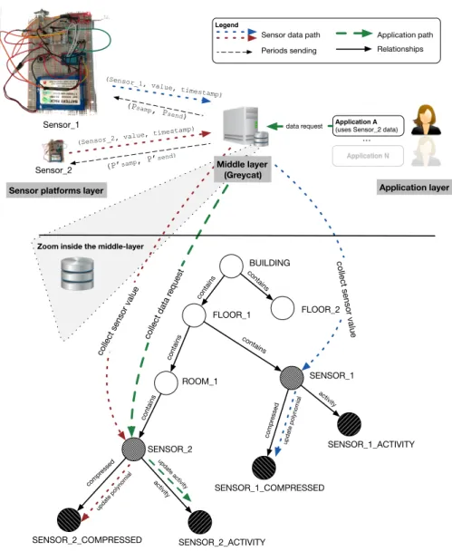
From the contributions presented in this section, we depict on Fig. 11 the implementation of the reference architecture presented in Fig. 5.
Sensor platforms layer. This layer contains all the sensor platforms targeted
by our approach. They execute an implementation of the adaptive firmware presented in Alg. 1. A server located in the middle layer is responsible to collect the sensor data and to compute the appropriate sampling and sending periods.
Middle layer. A server located in this middle layer is responsible for maintaining
the data structure presented in Fig. 6. Each time a sensor value is received from a sensor platform, the middle layer updates its corresponding nodes with the freshest value and foresees the next data sampling and sending periods. In
addition, for each periodic node, the middle layer updates the activity node each time a third-party application performs a sensor value request.
Applications layer. This layer contains the set of third-party applications that
retrieve sensor values.
Sensor_1
Sensor_2
(Psamp, P send)
(P’samp, P’send)
(Sensor_1, value, timestamp)
(Sensor_2, value, timestamp)
Application A (uses Sensor_2 data)
SENSOR_1_COMPRESSED SENSOR_1_ACTIVITY BUILDING FLOOR_1 FLOOR_2 ROOM_1 SENSOR_1 contains SENSOR_2 SENSOR_2_COMPRESSED SENSOR_2_ACTIVITY contains contains contains contains activity activity compr essed compr essed
collect sensor value collect data r
equest
collect sensor value
data request
update polynomial
update polynomial update activity
Zoom inside the middle-layer
Legend
Sensor data path Application path Periods sending Relationships
…
Sensor platforms layer
Middle layer (Greycat)
Application layer
Figure 11: Reference architecture for computing and sending adapted periods
5. Measuring the gain in battery lifetime
In the previous section, we have introduced a predictive model allowing the computation of adaptive sending and sampling periods based on the predicted values of the considered physical phenomena and on the predicted use of data by third-party applications. We focus in this section on measuring the gain in battery lifetime brought by this model (i.e., measuring aspect of our research question). We perform an experimental assessment on a prototypical sensor platform based on an ESP8266 microcontroller by conducting three experiments: • (Exp.1) aims at measuring the battery life-time of the sensor platform sampling and sending values at fixed periods without deep-sleep. The voltage at the moment the platform ceases to work will be considered as the cut-off voltage, i.e., the minimum voltage required by the platform to work properly. The following experiments will measure the time required to reach this value from a charged battery;
• (Exp.2) aims at measuring the time required to reach the cut-off value of the sensor platform sampling and sending values at fixed periods using deep-sleep. These values will be considered as reference values to measure the gain brought by our approach;
• (Exp.3) aims to empirically show that our approach increase the battery lifetime. Instead of fixing the periods, we use our contribution to dynam-ically compute adaptive sampling and sending periods.
5.1. Experimental setup
To perform the evaluation of the approach, we have instantiated the reference architecture (cf. Fig. 11) with the following elements:
Sensor platform layer. It contains platforms relying on an ESP8266
microcon-troller and on a temperature sensor. This microconmicrocon-troller is largely used by the IoT industry and offers an efficient deep-sleep mode, a Wi-Fi connectivity and a writable EEPROM that can be used to buffer data. In order to avoid any unwanted energy leaks, we have built an electronic design using the strictly nec-essary passive components. All the sensor platforms rely on a 3.7V 6000mAh lithium-ion battery.
Middle layer. It relies on a middleware9developed using Java 7 and Scala 2.11
languages and using the GreyCat technology. Greycat allows the middleware to trigger in a reactive way machine learning executions using the concepts presented in Sec. 2. The middleware builds automatically the prediction model presented in Sec. 4 and updates the nodes (cf. Fig. 6) each time a sensor value is collected.
Table 2: Initial settings for the 3 experimental contexts
Experiment Experiment Experiment
#1 #2 #3
Initial voltage (in V) 3.36 3.46 4.09
Period (in seconds) 150 150 adaptive
Deep-sleep 7 3 3 y = -16127x3+ 2966,9x2- 337,55x + 3375,1 R² = 0,9976 2800 2900 3000 3100 3200 3300 3400 3500 Ba tt er y v ol ta ge (i n m V) Running time (in days hours minutes) Battery discharge (Vinit = 3.36V / P=2min30 / without deep-sleep) Battery discharged
Figure 12: Battery dischargewithout deep-sleep (Exp.1)
Application layer. On this side, we have mocked an application behavior using
the collected temperature values.
For each experiment, we use a charged Li-ion battery and preconfigure, if necessary, the sampling/sending periods and the deep-sleep mode (cf. Tab. 2). 5.2. Standard battery discharge (Exp.1)
This first experiment aims to illustrate the lifetime of a battery-powered platform that does not use deep-sleep facilities nor adaptive periods. In order to conduct a time-limited experiment, we overexploit the platform by sampling and sending temperature values associated with the current voltage value at the battery terminals every 150 seconds. This value allows 24 measurments per hour simulating, at a speed increased by 24, a sensor performing one measurment per hour. Moreover, the undersampling of the voltage measurements mitigates the invasive effect of the measure, which also affect the battery.
The obtained voltage values are plotted on Fig. 12. We can observe that the voltage values decrease following a cubic function. The last value obtained
(∼ 3.0V ) corresponds to the cut-off value mentioned by the constructor [11] (i.e., the minimal voltage value for operating the platform) and has been reached
after Tcut= 8.5h. By extrapolating this result towards a platform that performs
only a single sampling and sending operation per hour (minimum requested, cf. hypothesis), i.e., the platform is used at a rate divided per 24, the battery
lifetime is then increased by 24 and reaches Tcut= 8.5days.
In our context (performing at least one measurement per hour), this shows that deploying such a battery-powered sensor platform without using deep-sleep facilities will lead to important maintenance operations as the battery will have to be replaced on a weekly-basis.
5.3. Battery discharge with deep-sleep (Exp.2)
The ESP8266 platform offers a deep-sleep facility that lowers the power consumption down to 10µA [11]. This second experiment aims at comparing the newly discharge curve with the one obtained in the first experiment in order to show how deep-sleep increase the platform lifetime. It also aims at showing whether the deep-sleep periods are sufficiently accurate regarding the periods desired by the user. For this experiment, we kept the same P = 150 seconds sampling/sending period as defined in Exp.1 and we enabled the deep-sleep facilities between two cycles.
The obtained voltage values are plotted on Fig. 13. To limit the experiment in time (an ESP8266 theoretically can stand for months using the deep-sleep facilities), we stopped the experiment before reaching the cut-off value. Despite some measurements artifacts (due to physicochemical properties of the battery - these artifacts, due to their low absolute value, are not representative), we observe that the curve follows a linear decrease (0.1V are lost every 2 days). From an initial voltage value of 3.46V , the extrapolation of the curve depicted in Fig. 13 shows that the cut-off value (3.0V ) is reached in 8 days. The application of the deep-sleep facilities to a platform performing only a single sampling and sending operation per hour can scale the battery lifetime up to 8 ∗ 24 = 192 days.
Through this experiment, we also wanted to check if the platform was cor-rectly inactive during deep-sleep periods, i.e., no sampling and sending oper-ations are performed and if the requested sleeping periods were correctly exe-cuted. We have thus extended the implementation of the algorithm presented in Alg. 1 to log on the serial port all the operations performed on the platform. Then, we have connected an oscilloscope to the output of the serial port and plotted the values obtained on the figure Fig. 14. The signal analysis shows a
platform stays woken-up (Tw1, Tw2, Tw3) 9 seconds on average (the connection
time to the wifi network is not deterministic and can therefore influence these
values) and sleeps (Ts1, Ts2) 145 seconds on average. Thus, an ESP8266
plat-form is active only 6% of a wake-up/sleep cycle. In particular, we notice that, as expected, no operations are performed during the deep-sleep. We can also
notice that the periods P1 and P2are close to the wished period of 150 seconds.
y = -6,5823x + 3366,1 3000 3050 3100 3150 3200 3250 3300 3350 3400 3450 00d 00:00 00d 12:00 01d 00:00 01d 12:00 02d 00:00 02d 12:00 03d 00:00 03d 12:00 Ba tt er y v ol ta ge (i n m V) Running time (in days hours minutes) Battery discharge (Vinit = 3.46V / P=2min30 / with deep-sleep)
Figure 13: Battery dischargewith deep-sleep (Exp.2)
650 700 750 800 850 900 950 1000 0, 08 11, 49 23, 02 34, 55 46, 08 57, 62 69, 14 80, 68 92, 2 103, 78 115, 45 127, 12 138, 79 150, 47 162, 14 173, 81 185, 48 197, 15 208, 82 220, 49 232, 16 243, 82 255, 5 267, 17 278, 83 290, 51 302, 18 313, 86 325, 52 337, 2 348, 87 360, 55 372, 22 383, 89 395, 57 407, 58 419, 25 430, 92 442, 59 454, 26 465, 93 Si gn al v al ue Time (in seconds) Sleep wake cycles Signal P1=155.02s Ts2=144.80s Tw1=8.81s Tw2=9.9s Tw3=8.9s Ts1=145.12s P2=153.7s
Figure 14: Wake-up/Sleep cycles(Exp.2)
Nevertheless, despite this slight imprecision, we can consider that the use of the deep-sleep respects the periods wished by the user.
5.4. Dynamic approach (Exp.3)
In this experiment, we propose to empirically show that adaptive periods contribute to increase the battery lifetime. We have implemented the firmware
Figure 15: Polynomials distribution. (Exp.3)
A dot represents the beginning time of a polynomial in its time-slot
presented in Alg. 110 and we have deployed it on our prototypical sensor
plat-form, as illustrated on the left hand-side of Fig. 11.
Set up. For this experiment, we set the following parameters :
• ∆t = 60 minutes in order to have at least one temperature measurement per hour.
• card(T ) = 24 in order to reason over a day.
• Precision of the prediction: 1 celsius degree to match the temperature sensor accuracy (which we consider as accurate enough for an office). 5.4.1. Sampling period
The computation of the appropriate sampling periods is performed accord-ingly to the polynomial functions computed by the compressed node To obtain initial polynomial functions, we fed the sensor node (cf. SENSOR on Fig. 6) with a 15 days dataset containing 3210 values and describing the temperature in the office under experiment. We configured the compressed node to accept
1.0celsius degree as an acceptable margin of error because of the accuracy of
the temperature sensor.
The polynomial regression performed by the compressed node results in 66 polynomials describing the learned data with a precision of 1.0 celsius degree. The figure Fig. 15 shows the number of polynomial function per time slot and their distribution within the time slot. The greater the number of polynomials in a given time slot, the more the physical phenomenon has changed and therefore
Figure 16: Computed daily sampling periods. During time-slot #10, the door is often closed, i.e., the temperature remains stable (Exp.3)
the sampling period must be reduced accordingly. According to this figure, we can observe that the most frequent changes occur during time slot #13. The more two beginnings of polynomials are separated in time, the more slowly the physical phenomenon varies. Thus, it is relevant to use the prediction result rather than to make an energy-intensive measurement. According to this figure, during time slot #0, we observe that the temperature varies slowly and, during time slot #16, the temperature fluctuates quickly. We report on Fig. 16, the
result of the sampling period computation from the application of Eq. 211
over the ∆ptvalues. When large temperature variations are expected to occur,
the sampling periods are decreased to ensure that the most data are sampled. Conversely, when the temperature is expected to remain stable, the sampling periods are increased to save the battery life-time.
In Tab. 3, we apply the polynomial segmentation on the datasets presented in Tab. 1 and extrapolate what would have been the autonomy of an ESP8266 platform considering a duty cycle of 9 seconds (cf. Fig. 14), an average op-erating current of 80 mA [11] and a 6000mAh 3.7V battery. Thanks to the polynomial segmentation algorithm, the number of values required to charac-terize a signal is greatly reduced (we showed in Sec. 3.1 that less than 10% of the values can describe the whole dataset). This reduction in the number of val-ues leads to greater deep-sleep periods (minimal operating current, ca. 20µA) and thus contributes to increasing the battery lifetime. By calculating the duty
11computing the set of minimal sampling periods P samp t∈T
Table 3: Theoretical gain in battery lifetime after using polynomial segmentation Sensor (compression) Duty cycle before comp. (s) Duty cycle after comp. (s) Estimated Battery lifetime (before comp., in days) Estimated Battery lifetime (after comp. in days) CAMPUS_TEMP (93%) 97.70 9.20 0.29 4.20 OFFICE_LIGHT (97%) 81.45 9.20 0.35 11.77 OFFICE_TEMP (97%) 81.42 9.20 0.35 11.77 CO_SENSOR (93%) 239.10 16.74 2.93 41.80 NOX_SENSOR (93%) 239.10 16.74 2.93 41.80 O3_SENSOR (92%) 239.10 19.13 2.93 36.57 NO2_SENSOR (92%) 239.10 19.13 2.93 36.57
cycle of the ESP8266 platform (9 seconds per data sampling and sending) be-fore compression and bringing it back to the battery capacity (6000mAh), the battery life for the datasets considered is between a few hours and a few days. After compression by segmentation, we change the scale for each of the consid-ered datasets: the battery lifetimes initially in hours become in days (or weeks), and the lifetime in days become months.
5.4.2. Sending period
The computation of the appropriate sending period is performed accordingly to the number of user requests and thus, as long as no data is requested by the users, it is irrelevant to establish an energy intensive data connection to send the values at high frequency. Nonetheless, they can be buffered locally, e.g., in the EEPROM memory of our setup, and sent when needed. Thus, the proposed optimization does not decrease the quality of data but only the latency to obtain it. As mentioned in Sec. 4, it is the responsibility of the activity node, i.e., a node using a time-slot storage to store the number of data accesses per time slot, to store the sensor activity.
We have mocked the sending periods displayed on Fig. 17. These periods allows to feed applications that needs to monitor the temperature during day-lights (time-slots 7 to 18) and more intensively around lunchtime, resulting in more requests during this period.
Figure 17: Computed daily sending periods (Exp.3)
For a time slot t ∈ T , the integer division of P sampt with P sendt returns
the number of data that is buffered on the platform between every sending. For example, from the periods depicted in Fig. 16 and Fig. 17, during time slot #1,
only one value will be buffered (P samp1 = 3600 and P send1 = 2894) before
being sent and during time slot #16, 39 values will be buffered (P samp16= 1800
and P send16 = 46) before being sent. This last value shows that 38 energy
intensive network connections have been saved thanks to buffering techniques during time slot #16.
5.4.3. Battery discharge
In this experiment, we have implemented the firmware described in Alg. 1 and deployed it on our prototypical platform. This platform retrieves the sampling and sending periods from the middle layer (cf. Fig. 11) and follows the values depicted respectively on Fig. 16 and Fig. 17.
Using such periods, the voltage values are plotted on Fig. 18. This figure shows that, among days and unlike Exp.1 and Exp.2, the voltage value at the battery terminals remains constant. Manual measurements using a voltmeter have shown that values under 4V are measurement artifacts. Comparing the battery discharge with the one observed in Exp.2 (cf. Fig. 13), we can deduce that adaptive periods allow us to extend the battery lifetime of our prototyping platform on a year scale.
0 500 1000 1500 2000 2500 3000 3500 4000 4500 00d 00:00 02d 00:00 04d 00:00 06d 00:00 08d 00:00 10d 00:00 Ba tt er y v ol ta ge (i n m V) Running time (in days hours minutes) Battery dischage (Vinit = 4.1V / adaptive periods / with deep-sleep)
Figure 18: Battery discharge using adaptive periods(Exp.3)
5.5. Summary
In this section, we have conducted an experimental validation to quantify the gain in battery lifetime brought about by the use of adaptive periods to answer the first part of the research question. For each experiment, we have measured the voltage at the battery terminals and compared the obtained values with respect to methods using static periods (with or without deep-sleep). We have seen that each of these experiments allowed us to change the battery lifetime scale: a weekly scale for fixed periods without deep-sleep, a monthly scale for fixed periods with deep-sleep, and finally an yearly scale for adaptive periods with deep-sleep. Moreover, the last experiment allows us to assess the accuracy of waking-up time when the sensor platform is in deep-sleep mode. We consider the time inaccuracy to be negligible in terms of impact on the battery lifetime. We consider these experiments to be relevant enough for measuring the gain in battery lifetime associated with the use of adaptive periods since we have compared three modes of operation: (i) fixed sending and samplig periods
with-outdeep-sleep, (ii) fixed sending and sampling periods with deep-sleep and (iii)
dynamic periods with deep-sleep. These experiments can be replicated on other platforms, provided they respect the prerequisites discussed in Sec. 4.
5.6. Threats to validity
Regarding measurements, voltage values were acquired by measuring the voltage at the battery terminals. These measures may be imprecise and must be considered noisy if taken as a whole. However, our study aims to measure a trend (increase or decrease) in battery life, which nuances this imprecision.
In addition, we have regularly confirmed the measured values with a digital multi-meter, confirming that the values obtained are close to reality.
Besides, some platforms integrate co-processors dedicated to specific func-tions (e.g., data acquisition) and designed to be energy efficient. For example,
ESP platforms integrate ULP12 (Ultra Low Power) coprocessors designed to
perform measurements using an ADC (Analog-Digital Converter), a temper-ature sensor and external sensors, while the main processor is in deep sleep mode. Our approach considers only the main processor and could be extended to benefit from these co-processors for the sampling. We expect this extension to significantly increase the battery lifetime gain obtained in our experiments. Conversely, badly designed deep-sleep modes and attached devices can overuse the battery and leak unnecessary energy limiting the gains made by activating deep-sleep mode and thus, the gains made by our proposed approach. Our con-tribution obviously exposes advantages and drawbacks of only interacting with devices through their deep-sleep mode interface. Still these devices are expected to well design their platform with regards to this mode.
Regarding the polynomial computation and re-training, these steps can af-fect system performance since it involves crossing the graph to retrieve the compressed node, read the current value and potentially update the polynomial or create a new timepoint if a significant change in data has been detected. To takle this issue, the middlelayer uses the GreyCat framework for storage and online learning. The evaluation of this framework performed in [30] showed
read and write throughputs close to 100, 000 nodes per second and a modify
throughput close to 400, 000 nodes per second. Hence, since a single physical sensor is described by three nodes (sensor node, activity node and compressed node, cf. Sec. 4.2), the approach can theoretically scale up to tens of thousands of sensors while having a re-training time of a few tens of millisseconds. 6. Related Work
In this work, we propose a cross-layer solution to reduce the energy consump-tion of a sensor platform. On the sensor platform layer, we rely on dynamic periods to sample and access the network. On the application layer, we rely on live machine learning techniques in order to not solicit the sensor network when values can be predicted. We have already introduced live machine learning in Sec. 2. In this section and with respect to our contributions, we compare in a first part, works addressing the dynamic periods problem before, in a sec-ond part, addressing MAC protocol optimizations and software-defined power meters. Then, we discuss machine learning techniques for forecasting data.
Dynamic periods. Dynamic periods can reduce the energy consumption by
sam-pling or sending sensor data only when needed. The approach proposed by Kho et al. [31] provides a decentralized control of adaptive sampling. They introduce
a metric based upon Fisher information and Gaussian process regression to de-fine three algorithms that compute a sampling period according to the gathered information. Alippi et al. [32] propose an algorithm that dynamically estimate a sampling period according to the observed signal. With this algorithm, they can minimize the activity of both the sensor and the radio, and thus, reducing the energy consumption. A simulation of this algorithm over a snow monitoring use case shows that up to 97% of the energy can be saved. More generally, the literature provides solutions based on gathered sensor measures to compute an adaptive sampling period [33]. However, they do not focus on applications’ re-quests. Whereas in our approach, we observe when data are requested in order to establish energy intensive network connections only when necessary.
MAC protocols. According to the IEEE 802 model, the Media Access Control
layer is responsible for network access. Numerous works have been achieved to reduce the energy footprint by defining energy-efficient MAC protocols. The T-MAC protocol [34] is a contention-based protocol for wireless sensor networks. It introduces an adaptive duty cycle relying on fine-grained timeouts and can save as much as 96% of the energy.
In our approach, in addition to reduce the network access with adaptive periods, we use the deep-sleep mode after every sending that shuts down the physical network interface and most of the sensor platform’s functionality, saving its energy
The DMAC protocol [35] uses the tree structure describing the major traffic schema in wireless sensor networks to optimize the energy. It schedules the activity of nodes according to their depth in the tree. Therefore, all the nodes on a multi-hop path can be notified of data delivering and can send their own measurements. Various experiments on this protocol have shown an energy saving of up to 6 times greater than conventional protocols. In our approach, we define a sending period for a single period but we reusing the concepts brought by DMAC by computing inter-platform dependent sending periods is a foreseen work.
Software-defined power meter. The WattsKit approach [36] aims at using
ma-chine learning methods to monitor the energy consumption of distributed sys-tems without the use of invasive and costly physical meters. To this end, the WattsKit approach profiles the electric consumption of some specific hardware operations such as CPU functions (e.g., TurboBoost, Hyper-threading) or device usages (e.g., Network, Disk). Based on these profiles, a model able to predict the overall hardware consumption from simple software probes is generated. During the training phase, a physical power meter is used, to obtain the real hardware power consumption and learn the expected impact of each function or device executions. Once the training phase is done, the model can be distributed over similar hardware without the need for physical meters. This model can be executed at run-time to build ultimately a software-sefined power meters that monitors the power consumption of an application (e.g., Apache ZooKeeper).
This software-defined power meter can be integrated into a higher-level applica-tion that can make decisions based on the identified energy consumpapplica-tion value (e.g., pause or delay the execution if a threshold value is exceeded). If their approach allows to obtain precisely the instantaneous power of a process (in Watt), they do not target microcontroller architectures mainly used within sen-sor networks. In our approach, we rely on the forecasting of data to reduce the energy consumption without the use of fine-grained prediction such as WattsKit. However, as future work, it would be relevant for a sensor platform to also use such approach and adapt its behavior according to the power required by the functions used on its hosted applications.
Forecasting data. Our approach heavily relies on a prediction model to evaluate
sensor value predictability. Due to our live usage of this prediction model, the ratio between its efficiency and effectiveness is key critical. For this reason we have selected polynomial functions for their excellent scalability. In [37], the authors show that polynomial functions achieve savings range from about 50% to 96%, according to the acceptable error threshold. However our contribu-tion can be extended by any other model offering similar performance tradeoffs. In particular various methods have been used for energy efficient sensor net-works [38]. The Least Men Square Algorithm [39] has been proposed to predict the measured values both at the sensor platform and remote levels. A trans-mission is performed only if the two predicted values differ from a variable step size. Such method offers the advantage to be simple enough to be embedded on restricted hardware, however without mid-term prediction they cannot drive deep-sleep operators like our contribution. Towards such goal, time series pre-diction models, as performed in our approach, give goods results to reduce the energy consumption. An adaptive model selection [37] applied on different data sets shows that despite the percentage of transmitted packets varying according to the algorithm used, they remain quite close. In our approach we rely on an polynomial regression model without memory which gives the fastest results according to the tested datasets.
7. Conclusion & Future work
In this paper, we have investigated whether one can significantly gain battery lifetime for a whole sensor platform using adaptive sampling and sending periods
(RQ).
To compute the adaptive sampling and sending periods, we have presented a self-adaptive approach using machine learning and deep-sleep to provide an optimal configuration extending the battery lifetime of a sensor platform. The generation of the optimal configuration is performed by a prediction model de-ployed on a middle layer located outside the sensor network. This middle layer receives sensor measures from remote sensor platforms and collect application’s requests on data (as shown on Fig. 11). According to historical values and current use of the sensor network, the middle layer foresees the next data sam-pling and sending periods. A firmware, deployed at the sensor platform layer,
requests the optimal configuration and buffers locally sensor data for a sending period.
Then, to measure the gain in battery lifetime, we have performed an experi-mental evaluation comparing the lifetime between a platform using fixed periods (with and without deep-sleep) and a platform using adaptive periods. Relying of these adaptive periods, we have successfully lowered the battery discharge. The extrapolation of the values obtained in our experiments showed us that an ESP8266 platform relying on a 6000 mAh battery could move from a weekly scale lifetime to a yearly scale lifetime thanks to adaptive periods.
The contribution of this paper relies on a regression model in order to eval-uate if sensor values can be extrapolated and to compute appropriate sampling and sending periods. The performance of this regression model directly impacts the energy reduction effect. Therefore in a future work, we plan to explore other learning methods, e.g., neural networks, and compare their efficiency towards this usage. In particular we will explore the impact of models with memory that can detect periodic patterns, such as LSTM networks [40]. In addition we also plan to work with unbounded time-slots, that describe better physical phenomena and reduce the number of computed polynomials.
Moreover, in this contribution we have optimized sensor periods indepen-dently. However, in case of sensors measuring the same phenomenon it could be highly beneficial to exploit the graph structure to generate optimal periods for a group of sensors (for instance, different sensors in a same room that provide comparable measurements). In such context, it might be interesting to synchro-nize the different sampling and sending values to orchestrate the measurement collection in turns, and thus not to always using the same sensors.
Finally, as many sensor platforms are nowadays available on the market with various capabilities for deep-sleep, we plan to assess our approach with different types of microcontrollers and architectures. Ultimately this would allow to classify their suitability towards such dynamic control usage.
Acknowledgements
This collaboration between Université Côte d'Azur and DataThings is sup-ported by the Doctoral Training programme of the European Institute of Tech-nology (EIT). The authors would also like to thanks Assaad Mowadad, Thomas
Hartmann, Gregory Nain and Matthieu Jimenez for their assistance with the
experimentations and for their comments that greatly improved this article. References
[1] A. H. Ngu, M. Gutierrez, V. Metsis, S. Nepal, Q. Z. Sheng, Iot middleware: A survey on issues and enabling technologies, IEEE Internet of Things Journal 4 (1) (2017) 1–20.
[2] S. Bandyopadhyay, M. Sengupta, S. Maiti, S. Dutta, A survey of mid-dleware for internet of things, in: Recent Trends in Wireless and Mobile Networks, Springer, 2011, pp. 288–296.
[3] C.-F. Chiasserini, M. Garetto, Modeling the performance of wireless sensor networks, in: INFOCOM 2004. Twenty-third AnnualJoint Conference of the IEEE Computer and Communications Societies, Vol. 1, IEEE, 2004. [4] R. Jurdak, A. G. Ruzzelli, G. M. O’Hare, Adaptive radio modes in sensor
networks: How deep to sleep?, in: Sensor, Mesh and Ad Hoc Communica-tions and Networks, 2008. SECON’08. 5th Annual IEEE CommunicaCommunica-tions Society Conference on, IEEE, 2008, pp. 386–394.
[5] A. Sharma, K. Shinghal, N. Srivastava, R. Singh, Energy management for wireless sensor network nodes, International Journal of Advances in Engineering & Technology 1 (1) (2011) 7–13.
[6] D. Lymberopoulos, A. Savvides, Xyz: a motion-enabled, power aware sen-sor node platform for distributed sensen-sor network applications, in: Proceed-ings of the 4th international symposium on Information processing in sensor networks, IEEE Press, 2005, p. 63.
[7] E. Shih, S.-H. Cho, N. Ickes, R. Min, A. Sinha, A. Wang, A. Chandrakasan, Physical layer driven protocol and algorithm design for energy-efficient wireless sensor networks, in: Proceedings of the 7th annual international conference on Mobile computing and networking, ACM, 2001, pp. 272–287. [8] B. Hohlt, L. Doherty, E. Brewer, Flexible power scheduling for sensor net-works, in: Proceedings of the 3rd international symposium on Information processing in sensor networks, ACM, 2004, pp. 205–214.
[9] S. Bi, C. K. Ho, R. Zhang, Wireless powered communication: opportunities and challenges, IEEE Communications Magazine 53 (4) (2015) 117–125. [10] Z. Xiao, W. Song, Q. Chen, Dynamic resource allocation using virtual
machines for cloud computing environment, IEEE transactions on parallel and distributed systems 24 (6) (2013) 1107–1117.
[11] Esp8266ex datasheet.
URL https://www.espressif.com/sites/default/files/
documentation/0a-esp8266ex_datasheet_en.pdf
[12] D. J. Hand, Principles of data mining, Drug safety 30 (7) (2007) 621–622. [13] D. A. Dickey, W. A. Fuller, Distribution of the estimators for autoregressive time series with a unit root, Journal of the American statistical association 74 (366a) (1979) 427–431.
[14] O. Anava, E. Hazan, S. Mannor, O. Shamir, Online learning for time series prediction., in: COLT, Vol. 30, 2013, pp. 172–184.