Computational Investigation of the Thermal Conductivities
and Phonon Properties of Strontium Cobalt Oxides
by
Hantao Zhang
B.S. Applied Physics, University of Science and Technology of China, 2016
Submitted to the Department of Nuclear Science and Engineering in Partial Fulfillment of the Requirements for the Degree of
Master of Science in Nuclear Science and Engineering
at the
Massachusetts Institute of Technology
June 2019
© 2019 Massachusetts Institute of Technology. All rights reserved.
Signature of Author: _____________________________________________________ Department of Nuclear Science and Engineering
May 17, 2019 Certified by: ___________________________________________________________ Bilge Yildiz Professor of Nuclear Science and Engineering, and Professor of Materials Science and Engineering Thesis Supervisor Certified by: ___________________________________________________________ Gang Chen Carl Richard Soderberg Professor of Power Engineering Thesis Reader Accepted by: ___________________________________________________________
Ju Li Battelle Energy Alliance Professor of Nuclear Science and Engineering, and Professor of Materials Science and Engineering Chairman, Committee for Graduate Students
3
Computational Investigation of the Thermal Conductivities
and Phonon Properties of Strontium Cobalt Oxides
by
Hantao Zhang
Submitted to the Department of Nuclear Science and Engineering on May 17, 2019 in Partial Fulfillment of the
Requirements for the Degree of Master of Science in Nuclear Science and Engineering
ABSTRACT
The thermal conductivities of electrochemically tuned strontium cobalt oxides (SCO) are significantly different among the perovskite SrCoO3 (P-SCO), the brownmillerite
SrCoO2.5 (BM-SCO) and the hydrogenated HSrCoO2.5 (H-SCO)1. The underlying
mechanism causing this large difference is still unclear. And phonon properties in SCO have not been investigated thoroughly or have some contradictive predictions. In this work, we have calculated the thermal conductivities in P-SCO and BM-SCO by applying molecular and lattice dynamics, and successfully reconstructed the large difference of the thermal conductivities, consistent with measurements. Furthermore, several phonon properties including heat capacities, group velocities, lifetimes and mean free paths have been calculated, and the key roles of local atomic environment and crystal symmetry in determining the thermal conductivities have been identified.
We have also analyzed the impact of interfaces, isotropic strains and defects on thermal conductivities, predicted the neutron scattering intensity in P-SCO, and tested the accuracy and performance of molecular dynamics based on deep learning. Additionally, even though the calculations about the phonon properties in H-SCO are not complete, it still offers some inspirations about its thermal conductivity. The thorough investigations about the phonon properties and the mechanisms determining the thermal conductivities in SCO may benefit future research about tunable thermal conductivities in complex oxides.
Thesis Supervisor: Bilge Yildiz
Title: Professor of Nuclear Science and Engineering, and of Materials Science and Engineering
Thesis Reader: Gang Chen
5
ACKNOWLEDGMENTS
Firstly, I would like to sincerely express my great gratitude to my academic advisor, Prof. Bilge Yildiz. Without her generous help, her patience and her wise knowledge, this work could not be initiated and completed.
Besides, I really appreciate the academic advising and suggestions from Prof. Gang Chen. His suggestions help me overcome many challenging problems during this project.
I greatly appreciate the financial support from MIT MRSEC through the MRSEC Program of the National Science Foundation under Award No. DMR-1419807, and from the McCormick Fellowship at MIT. Also, I want to acknowledge the computational resource support from the National Energy Research Scientific Computing Center, the Plasma Science and Fusion Center and Department of Nuclear Science and Engineering at MIT, and the Extreme Science and Engineering Discovery Environment at Texas Advanced Computing Center.
In addition, I would like to specially thank Qichen Song. Our close collaboration produces many interesting results and exciting ideas. Also, I learn quite a lot from his great passion about science, and his encouragement relieves me during my hard time.
I also would like to thank Dr. Olle Hellman, Dr. Terumasa Tadano, Jing Yang, Dr. Lixin Sun, Dr. Franziska Hess, Yen-ting Chi, Minh Dinh, Vrindaa Somjit, Prof. Rafael Gomez-Bombarelli, Wujie Wang, Zhe Shi, Dr. Qiyang Lu, Xiang Chen, Haowei Xu and many other colleagues and friends, for their technical help and fruitful discussion.
Finally, I would like to express my great gratitude to my parents. They always encourage and help me when I am facing difficulty and frustration. I am very fortunate to have a supportive family.
7
CONTENTS
ABSTRACT... 3
ACKNOWLEDGMENTS ... 5
1. Introduction ... 9
2. Theory and Methodology ... 11
2.1. Phonon and phonon transport ... 11
2.2. Phonon linewidth and phonon-neutron scattering cross section ... 16
2.3. Boundary and interfacial impact on thermal conductivity ... 17
2.4. Phonon-defect scattering ... 20
2.5. DDEC6 net atomic charge and bond order ... 22
2.6. Strain effect on thermal conductivity... 24
2.7. Molecular dynamics based on deep learning ... 25
2.8. Computation Details ... 26
3. Results and Discussion ... 29
3.1. Structure parameters, electronic and magnetic properties of SCO ... 29
3.2. Phonon properties and thermal conductivities in SCO ... 32
3.2.1. Second-order and third-order force constants, net atomic charges and bond orders in P-SCO and BM-SCO ...32
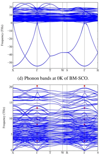
3.2.2. Phonon dispersion relationships and density of states in P-SCO and BM-SCO ...38
3.2.3. Thermal conductivities at 300K in P-SCO and BM-SCO ...41
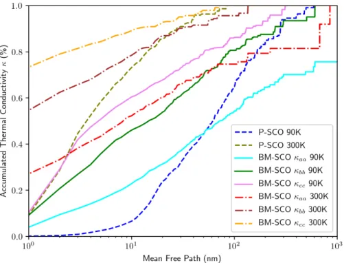
3.2.4. Accumulated thermal conductivities in P-SCO and BM-SCO ...45
3.2.5. Frequency spectrums of the thermal conductivities in P-SCO and BM-SCO ...46
3.2.6. Probability density distributions of phonon properties in P-SCO and BM-SCO...48
3.2.7. Temperature dependence of heat capacities in P-SCO and BM-SCO ...51
8
3.2.9. Thermal conductivity predicted by the pure defect scattering model in the oxygen
deficient P-SCO ...57
3.2.10. Predicted neutron scattering intensity at 300K in P-SCO ...60
3.3. The effect of isotropic strains on thermal conductivities of P-SCO ... 61
3.3.1. Thermal conductivity in the isotropically strained P-SCO ...61
3.3.2. Phonon dispersion relationship and density of states in the strained P-SCO ...64
3.3.3. Temperature dependence of heat capacity in the strained P-SCO ...66
3.3.4. Probability density distributions of phonon properties in the strained P-SCO ...67
3.3.5. Frequency spectrums of phonon properties in the strained P-SCO ...70
3.4. Interfacial effect on the thermal conductivities of P-SCO and BM-SCO ... 73
3.5. Test of DeepMD in calculating phonon properties... 76
3.5.1. Comparison of structural calculations in P-SCO from DeepMD and AIMD ...76
3.5.2. Comparison of phonon properties in P-SCO from DeepMD and AIMD ...78
3.6. Phonon dispersion relationship in H-SCO ... 81
4. Conclusions ... 83
9
1. Introduction
Thermal conductivity determines the efficiency of heat transport in materials. This property is important for microelectronic devices2 and thermoelectric energy conversion
devices3,4, where the nanoscale electronic chips require high conductivity to avoid
overheating while the thermoelectric devices require low conductivity. These different requirements may be demanded simultaneously in a single device like an “electrical heat valve”. In this case the tunability of thermal conductivity via applied electric field is desirable.
Recent studies showed that electrochemical insertion of lithium ions into graphite5 and
MoS26can tune thermal conductivity down to 2-3 folds. In principle, the inserted ions
(serving as point defect sites) can scatter phonons and electrons which act as heat carriers, leading to thermal conductivity reduction3. Importantly, our recent experimental
investigation on insertion and removal of oxygen and hydrogen ions into and from SrCoOx
(denoted as SCO) achieved a larger range of tunability of thermal conductivity1.
In our group, we have studied the thermal conductivity of the perovskite phase SrCoO3-δ (denoted as P-SCO and δ means oxygen nonstoichometry), the brownmillerite phase SrCoO2.5 (denoted as BM-SCO), and the hydrogenated strontium cobalt oxide
HSrCoO2.5 (denoted as H-SCO). We found that the insertion and removal of oxygen and
hydrogen ions can reversibly change thermal conductivity up to an unprecedented 15 folds, among BM-SCO, P-SCO and H-SCO phases1. The key behind this large range of tunability
is the ability to span electrically across multiple phases and a wide range of electronic conductivities with multiple ions. On the other hand, previous tunable thermal conductivity of Li+ inserted MoS
26 and Si-Ge alloy7 involved single phase and single ion. Moreover,the
drastic change of thermal conductivities in three phases with a large electrical property difference shows a potential of thermoelectric applications.
The electrochemical transformation involves three phases, two ions, and transition between conductors and insulators. As a result, the concentration of impurities and electronic carriers, and crystal symmetries vary simultaneously. This makes it difficult to identify underlying thermal transport mechanisms. Experimental work is not sufficient to capture phonon behavior and properties, so first-principles calculations for P-SCO, BM-SCO and H-BM-SCO about phonons are needed. With this computational work of phonon scattering, we can deeply understand the dominant mechanisms behind our experimental results, and this knowledge can be utilized to design more novel materials with tunable thermal conductivity, which can benefit advanced electronics.
11
2. Theory and Methodology
2.1. Phonon and phonon transport
In solid crystals, atoms occupy and vibrate around their equilibrium positions. The decomposed vibrations of all atoms in each single frequency harmonic mode can be described in a quantum mechanical way, that is phonon. To study phonon, interatomic interactions should be clarified. During atomic motions, the difference between atomic position and the equilibrium position of atom α in the 𝐴th cell in the direction of 𝑖 is labeled as a displacement 𝑢'(). Usually the displacement is very small, so we can express the interatomic potential as a Taylor expansion around the equilibrium position. In this sense, the effective Hamiltonian can be written as8,9
𝐻 = 𝑇 + 𝑈 = ∑ 𝐩123
452
') + 𝑈6+74∑'9);(:Φ'9(:); 𝑢'()𝑢9:; +<7∑'9=);?(:>Φ'9=(:>);? 𝑢'()𝑢9:;𝑢=>? + ⋯, ( 1 )
where 𝑇 and 𝑈 are the kinetic energy and potential energy, 𝐩') and 𝑚) are the momentum and mass of atom α in the 𝐴th cell, 𝑈6 is the equilibrium potential energy, Φ'9(:); and Φ'9=(:>);? are the second-order and third-order interatomic force constants. In principle, we can expand the effective Hamiltonian to infinite order terms, but usually only low-order terms have dominant impacts on phonon properties and high-order terms are very challenging for phonon computations, so in this work we just focus on second-order and third-order terms. Since we drop high-order terms but we still need high accuracy and temperature effect, we can effectively take all high-order terms into second-order and third-order terms, making them temperature dependent. In this case, 𝑈 = 𝑈(𝑇) and this is called the temperature dependent effective potential (TDEP)9,10. In practice, to obtain the
temperature dependent potential energy, molecular dynamics9,10 or stochastic sampling
method11,12 can be applied. After sampling, fitting of atomic forces and displacements gives
the force constants9,
𝐹() = ∑ Φ 69(: ); (𝑇) ∙ 𝑢
9:;
9;: +74∑9=;?:>Φ69=(:>);? (𝑇) ∙ 𝑢9:; 𝑢=>? . ( 2 )
With these force constants, we can proceed to phonon and thermal conductivity calculations.
According to the definition of phonon, second-order force constants determine harmonic phonon properties, and with them we can represent second-order force constants in the Fourier space as8,13,14
12
ΦF(𝐪)(:); = ∑ Φ'9 '9(:); 𝑒(𝐪∙(𝐑1J𝐑K), ( 3 )
where 𝐑' and 𝐑9 are the translation vectors of cell 𝐴 and 𝐵 . From this Fourier representation, the dynamical matrix 𝐷F(𝐪)(:); can be constructed as8,13,14
𝐷F(𝐪)(:); = NF (𝐪)OP2Q
R525Q . ( 4 )
The eigenvalues 𝜔(𝐪:) and eigenvectors 𝒆)(𝐪:) of the dynamical matrix correspond to the frequencies and polarization vectors of phonon mode 𝑗, which can be written as8,14
∑ 𝑫FW𝐪:X);𝒆;(𝐪:)
; = 𝜔4(𝐪:)𝒆)(𝐪:). ( 5 )
After obtaining phonon frequency 𝜔(𝐪:) , the group velocity of phonon mode 𝑗 is 𝒗W𝐪:X = Z[(𝐪P)
Z𝐪P which is necessary for phonon transport calculations.
Usually, modeling atomic interactions as neighboring atoms’ harmonic interactions is not enough for practical computations. One big error is from the anharmonic nature of atomic interactions, which will be discussed later. Another error comes from the long-range Coulombic interactions. In a practical phonon model, interatomic interactions are considered as short range with some distance cutoff. In polar materials, the displacements of atomic positions can lead to the formation of dipoles15 . This kind of nuclei displacement
induced dipole-dipole interaction follows Coulomb’s law, and the formed polarization per unit cell along direction 𝑖 is proportional to the atomic displacement along direction 𝑗 with the coefficient, Born effective charge, 𝑍(:∗ 13,15. This dipole-dipole interaction is
related to the LO-TO splitting of the phonon frequency at the Brillouin zone’s center13,15.
To capture this long-range effect, a non-analytic correction to the dynamical matrix in the first Brillouin zone can be16,
𝐷F^_^`a(𝐪)(:); = 𝐷F6(𝐪) (: ); + bcd3 eR525Q∙ [𝐪∙𝐙2∗]Oi𝐪∙𝐙Q∗jP 𝐪∙kl∙𝐪 ∙ exp (− 𝐪3 q), ( 6 )
where 𝐷F6(𝐪)(:); is the uncorrected dynamical matrix, 𝑒 is the electron charge, 𝑉 is the volume of the primitive cell, 𝐙)∗ is the Born effective charge tensor of atom 𝛼, 𝜖u is the
dielectric constant tensor, and 𝜎 is the damping factor which is a free parameter to make the non-analytic correction vanish at the Brillouin zone’s boundary. The Born effective
13
charge tensors and dielectric constant tensor can be obtained from experiments or first-principles calculations.
In the model of harmonic potential, crystal vibrations are the summation of individual phonon modes, and each phonon mode has no relation with others. In this case, phonons transport in perfect crystals without collisions, resulting in infinite thermal conductivity. However, in a real solid, lattice thermal conductivity is limited, so the consideration of phonon coupling and phonon collision is necessary. Phonons are coupled due to anharmonic force constants, and in high temperature regimes the most dominant contribution to phonon collisions in perfect crystals is from three-phonon scattering determined by third-order force constants. To characterize the strength of three-phonon scattering events, three-phonon scattering matrix is14,17
ΦFW𝐪w, 𝐪y, 𝐪zX = ∑ dO2(𝐪{)dPQ(𝐪|)d}~(𝐪•)
R525Q5~ Φ'9=(:>
);? 𝑒((𝐪{∙𝐑
1J𝐪|∙𝐑KJ𝐪•∙𝐑€)
'9=(:>);? . ( 7 )
The strength of phonon scattering is also represented in the phonon lifetime: the stronger scattering is, the shorter a phonon can live. The phonon lifetime is determined by the imaginary part of phonon self-energy8,9,17
7
•{= 2Γw, ( 8 )
where 𝜏w and Γw are the lifetime and the imaginary part of self-energy of phonon mode 𝜆 , respectively. The imaginary part of self-energy is associated with three-phonon scattering matrix by14,17 Γw = ∑ ℏc 7‡ˆ‰[(𝐪{)[(𝐪|)[(𝐪•)|ΦFW𝐪 w, 𝐪y, 𝐪zX|4× [2W𝑛(𝐪y) − 𝑛(𝐪z)X𝛿 Ž𝜔W𝐪wX + yz 𝜔(𝐪y) − 𝜔(𝐪z)• + W1 + 𝑛(𝐪y) + 𝑛(𝐪z)X𝛿 Ž𝜔W𝐪wX − 𝜔(𝐪y) − 𝜔(𝐪z)•], ( 9 ) where 𝑛(𝐪y) = 7 d ℏ‘(𝐪|) }K’ “7
is the Bose-Einstein distribution function representing the average occupation number of phonon mode 𝐪y, and 𝑁6 is the total number of phonon modes in the first Brillouin zone. Due to the requirement of momentum conservation, the wave vectors of three phonons must have
𝐪w + 𝐪y + 𝐪z = 0 or 𝐆, ( 10 )
where 0 corresponds to the normal scattering, and 𝐆, a reciprocal space lattice vector, corresponds to the umklapp scattering. Usually the umklapp scattering is dominant, so here we focus on the umklapp three-phonon scattering.
14
After obtaining the phonon lifetime, we can consider phonon flow carrying heat. The heat flow carried by phonon flow is18
𝐽( = e7∑ 𝑛w ˜W𝐪wXℏ𝜔W𝐪wX𝑣(W𝐪wX, ( 11 )
where 𝑛˜W𝐪wX and 𝑣(W𝐪wX are the non-equilibrium distribution function and the group velocity along direction 𝑖 of phonon mode 𝐪w, respectively. If the temperature gradient is small, we can expand the non-equilibrium distribution function of one phonon mode around the equilibrium distribution 𝑛18,
𝑛˜ = 𝑛 +š› š𝐫 ∙ 𝑑𝐫 = 𝑛 + š› šž∙ ∇𝑇 ∙ 𝑑𝐫 = 𝑛 + š› šž∙ ∇𝑇 ∙ 𝐯 ∙ 𝜏, ( 12 )
where 𝐯 is the phonon group velocity, 𝜏 is the phonon mean lifetime. We can plug it into the non-equilibrium distribution expansion,
𝐽( = 7 e∑ [𝑛W𝐪 wX +š› šž∙ ∇𝑇 ∙ 𝐯(𝐪 w) ∙ 𝜏(𝐪w)]ℏ𝜔W𝐪wX𝑣 (W𝐪wX w . ( 13 )
The equilibrium distribution cannot contribute to the heat flow, therefore 𝐽( =∇že ∙ ∑ š›šž∙ 𝐯(𝐪w) ∙ 𝜏(𝐪w) ∙ ℏ𝜔W𝐪wX𝑣
(W𝐪wX
w = (𝜿 ∙ ∇𝑇)(. ( 14 )
Comparing the heat flow expression of phonon and Fourier’s law, we know (𝜿 ∙ ∇𝑇)( = ∑ 𝜅: (: ∙ ∇𝑇: = ∑ e7∑ š›
šž∙ 𝑣:(𝐪w) ∙ 𝜏(𝐪w) ∙ ℏ𝜔W𝐪wX𝑣(W𝐪wX
w ∙ ∇𝑇:
: , ( 15 )
then the thermal conductivity tensor 𝜅(: is8,17,18
𝜅(:=e7∑wš›šž∙ ℏ𝜔 ∙ 𝜏W𝐪wX ∙ 𝑣(W𝐪wX𝑣:W𝐪wX=e7∑ 𝐶w e(𝜔w, 𝑇) ∙ 𝜏w(𝑇) ∙ 𝑣(w∙ 𝑣:w. ( 16 )
Here 𝜆 means each phonon mode, 𝐶e is the phonon heat capacity with 𝐶e = (ℏ[) 3 >Kž3 7 ¤d ℏ‘ }K’“7¥ 3𝑒 ℏ‘ }K’. ( 17 )
Because calculating thermal conductivity needs to sample the Brillouin zone, a finite Brillouin zone mesh can lead to errors in calculations. To compensate this artifact effect, the thermal conductivity is extrapolated to an infinite mesh size through19
15 ¦§}(ž) ¦l(ž) = 1 − ¨(ž) ›} + 𝑂( 7 ›}3), ( 18 )
where 𝑛> is the number of sampling points along one dimension of the mesh, 𝜅›} is the
thermal conductivity calculated on this mesh, 𝜅u is the extrapolated thermal conductivity, 𝑐 is a temperature-dependent coefficient. By calculating thermal conductivities on different meshes, we can fit thermal conductivities with different mesh sizes and obtain 𝜅u.
It should be noted that in this study, the temperature-dependent thermal conductivity is modeled by taking the temperature-dependent phonon heat capacity and intrinsic phonon-phonon scattering rates into account. The lattice parameters, crystal structures, and phonon dispersion relationships are still assumed to be the same as those at 300K. This assumption is made to avoid extensive computation of molecular dynamics at different temperatures, and it should have negligible impact within the temperature regime close to 300K. The thermal expansion coefficient of P-SCO is around 13 × 10“‡/K near 300 K20.
With the temperature variation of 100 K, the change of lattice parameters is smaller than 0.13%, and this small change of lattice parameters would cause the variation of thermal conductivity less than 4% estimated from the linear trend of thermal conductivity with respect to isotropic strain. Therefore, it is reasonable to make this assumption. Phonon heat capacities, and rates of intrinsic phonon-phonon scattering with cubic anharmonicity, depend on the temperature, and these lead to the temperature dependence of thermal conductivities in our calculations.
To characterize the impact of crystal symmetry on the phonon scattering channels, we calculate the three-phonon scattering phase space. The definition of total three-phonon scattering phase space 𝑃< is21,
𝑃<= ˆ7 -∑ 𝑃<W𝐪 wX w , ( 19 ) 𝑃<W𝐪wX = 7 <53i2𝑃<(J)W𝐪wX + 𝑃<(“)(𝐪w)j, ( 20 ) 𝑃<(±)W𝐪wX = 7 ˆ-∑ 𝛿 Ž𝜔W𝐪 wX ± 𝜔(𝐪y) − 𝜔(𝐪z)• 𝛿W𝐪w± 𝐪y− 𝐪z − 𝐆X y,z , ( 21 )
where 𝑚 is the number of phonon branches, 𝑁¯ is the number of q points in the reciprocal space, 𝐆 is the reciprocal space lattice vector. The definition of the scattering phase space is similar to the definition of the imaginary part of phonon self-energy, while the difference is that no three-phonon scattering matrix and no phonon occupation number are involved in the scattering phase space’s definition. The physical meaning of scattering
16
phase space is that it counts all possible phonon decay channels. With larger scattering phase space, there exist more three-phonon decay channels.
2.2. Phonon linewidth and phonon-neutron scattering cross section
In the previous discussion, we have treated the anharmonic Hamiltonian in a perturbative way, which means that we model the anharmonic lattice vibrations in the quasi-particle picture of phonons with phonon-phonon interactions. In this scenario, phonon is an eigenstate of harmonic Hamiltonian, not of anharmonic Hamiltonian. According to the perturbation theory, the eigenstate of perturbed Hamiltonian is approximately the linear combination of original eigenstates, and the original unperturbed eigenstate decays into other eigenstates with time evolution22. This leads to the fact that in
anharmonic crystals, physical vibration frequencies, or eigenvalues of perturbed Hamiltonian, are not the same as harmonic vibration frequencies or phonon frequencies but with shifts, and harmonic phonons are no longer stationary but with finite lifetimes and frequency broadening23,24. To characterize this effect, we first need to compute the phonon
self-energy Σ of mode 𝜆 as23
Σw = Δw + 𝑖Γw. ( 22 )
The imaginary part of the self-energy Σw, Γw, has already been given in the thermal conductivity calculations. Then the real part of self-energy Δw can be obtained by the Kramers-Kronig transformation23,25,26
Δw(Ω) = 7
c∙ 𝑃𝑉 ∙ ∫ ´{([)
[“µ 𝑑𝜔. ( 23 )
Here 𝑃𝑉 denotes the Cauchy principal value. When doing any resonance experiments, the actual measured frequency Ω should be23
Ω4 = 𝜔4W𝐪wX + 2𝜔W𝐪wXΔW𝐪w, ΩX. ( 24 )
We can clearly see that stronger anharmonicity leads to larger Γw meaning shorter lifetime, and larger Γw leads to larger Δw meaning larger measured frequency shift. Apart from frequency shift, phonon frequency broadening can be considered in the following way: phonons scatter with incident photons or neutrons in Raman or neutron scattering measurements. The cross section of scattering with phonon mode 𝐪w reflects the distribution of phonon frequency Ω as23,25
𝜎W𝐪w, ΩX ∝ 4[W𝐪{X´(𝐪{,µ)
17
In harmonic crystals, self-energy Σ = 0, therefore this cross section reduces to the Dirac δ function with a peak of Ω = ωWq½X; In anharmonic crystals, the self-energy gives a finite linewidth, and stronger anharmonicity leads to broader frequency distribution. It’s worth noting that this kind of frequency shifting and broadening is not unique in phonon systems and it also exists in electron systems. Electron energy in the angular-resolver photoemission spectroscopy (ARPES) also shows similar shifting and broadening due to electron-electron and electron-phonon interactions26–28.
Since both P-SCO and BM-SCO have magnetism, the spin-neutron interaction can be another factor contributing to the total scattering cross section. Therefore, the cross section of neutron scattering we focus on in this work only includes the phonon-neutron part. 2.3. Boundary and interfacial impact on thermal conductivity
Thermal conductivity in high temperature regimes is usually dominated by phonon-phonon scattering18, which has been discussed above. Phonon-phonon scattering scales
thermal conductivity with temperature as 𝜅¾¿“¾¿~7ž18,19, and this relationship diverges
near 0K. It is unphysical to have a diverging natural quantity, thus some other scattering mechanisms including boundary and defect scattering should also be considered in low temperature regimes. We first focus on the boundary or finite size effect.
Boundary scattering is usually accurately calculated by solving the Boltzmann Transport Equation (BTE)18, which requires cumbersome mathematical tricks or complex
numerical simulations. To qualitatively estimate the importance of boundary effect in our problem, we start from a very simple model inspired by Fuchs’s treatment of electron transport in a thin film29.
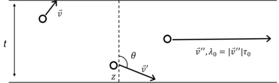
Fig. 1. Boundary scattering in the thin film. Circles denote phonons, 𝑡 is the film thickness, 𝑣⃑, 𝑣⃑˜ and 𝑣⃑′′ are phonon group velocities, 𝜆
6 is the phonon bulk mean free path, 𝜏6 is the phonon bulk mean lifetime, 𝑧 is the vertical distance between the phonon and the bottom interface, and 𝜃 is the angle between the group velocity and the cross-plane direction.
18
We construct a model for a thin film with a thickness of 𝑡 along 𝑧 direction and an infinite size along 𝑥 and 𝑦 directions, which is shown in Fig. 1. Phonon intrinsic properties in the film, including dispersion relationship, density of states, group velocities, mean free paths and mean lifetimes, are still the same as those in bulk materials. When a phonon travels to the film boundary, it annihilates and a new phonon is created independently with an isotropic traveling direction. This assumption indicates the diffuse boundary30. Our model is similar to McGaughey’s one30, but we treat every phonon mode
independently and without the assumption of single acoustic phonon branch. 𝑧 axis is constructed along the cross-plane direction, and 𝑧 = 0, 𝑧 = 1 denote the bottom and top interface of the film respectively. A phonon is created inside the film with a position 𝑧, and a direction 𝜃 which is the angle between the group velocity and 𝑧 axis. If the phonon mean free path in bulk materials is 𝜆6, then the free path in the film 𝜆 would be
𝜆 = ⎩ ⎪ ⎨ ⎪
⎧𝜆6, 𝜃 <c4 and 0 < 𝑧 < 𝑡 − 𝜆6𝑐𝑜𝑠𝜃, or 𝜃 > c4 and − 𝜆6𝑐𝑜𝑠𝜃 < 𝑧 < 𝑡 ^“Ð ¨_ÑÒ, 𝜃 < c 4 and 𝑡 − 𝜆6𝑐𝑜𝑠𝜃 ≤ 𝑧 < 𝑡 −¨_ÑÒÐ , 𝜃 >c4 and 0 < 𝑧 ≤ −𝜆6𝑐𝑜𝑠𝜃 . ( 26 )
If the temperature gradient across the film is very small, we assume the phonon creation position is uniformly distributed along 𝑧 axis, so creation at the position 𝑧 has the probability of 𝑝(𝑧) =7^, 0 < 𝑧 < 𝑡, and the mean free path in the film 𝜆̅ becomes
𝜆̅ = ∫ 𝜆𝑝(𝑧)𝑑𝑧6^ . ( 27 )
Given the relation of 𝜆̅ = |𝒗|𝜏̅ and •Ö
•‰=
w×
w‰, where 𝒗, 𝜏̅ and 𝜏6 are the phonon group
velocity, the mean lifetime in the film and the mean lifetime in bulk materials respectively, we can obtain the formula of mean lifetimes in the film,
𝜏̅ = ⎩ ⎪ ⎨ ⎪ ⎧𝜏6Ž1 − Øw‰¨_ÑÒ4^ Ø• , if 𝜆6 ≤ ب_ÑÒ^ Ø 𝜏6Ø4w ^ ‰¨_ÑÒØ , if 𝜆6 > Ø ^ ¨_ÑÒØ 𝜏6, if 𝜃 =c4 . ( 28 )
In this case, the thermal conductivity formula is modified to 𝜅(: = 7
e∑ 𝐶e(𝜔
w, 𝑇) ∙ 𝜏̅
filmw ∙ 𝑣(w ∙ 𝑣:w
19
where 𝜏̅filmw is the effective mean lifetime of the phonon mode 𝜆 in the film.
It should be pointed out that this model has its limitations, that implicitly the temperature gradient across the film is assumed to be small and negligible, and that the thermal conductivity calculated here only reflects the near-equilibrium state. If the temperature gradient is large, this model must be modified.
Since a SCO film is deposited on a substrate and coated with an Al film1, the
time-domain thermoreflectance (TDTR) signal reflects the total thermal conductivity across the whole structure, and it is hard to separate the interfacial thermal conductivity from the total one with certainty. It would be valuable to model and calculate the total thermal conductivity and the interfacial one. In this work, the interfacial thermal conductivity, or the interfacial thermal resistivity, is modeled by the diffuse mismatch model (DMM) 18,31,32
and the acoustic mismatch model (AMM) 18,32, and the total thermal resistivity 𝑅
^_^`a is
the summation of two interfacial thermal resistivities 𝑅(›^dÚÛ`¨d,7 and 𝑅(›^dÚÛ`¨d,4, and the SCO thermal resistivity 𝑅Ü=Ý,
𝑅^_^`a = 𝑅(›^dÚÛ`¨d,7+ 𝑅(›^dÚÛ`¨d,4+ 𝑅Ü=Ý, ( 30 )
which is also used in prior experimental work33,34.
In DMM, when phonons elastically collide with boundaries, they are absorbed and then reflected or transmitted isotropically without any memory of polarizations and directions31. The transmission probability from side 1 to side 2 is given by31
𝛼7(𝜔) = ∑ ÞP 3,Pß3,P([)
∑ ÞP 3,Pß3,P([)J∑ ÞP à,Pßà,P([)=
∑ ÞO 3,O
∑ ÞO 3,OJ∑ ÞP 3,O , ( 31 )
where 𝜔 is the phonon frequency, 𝑗 is the phonon branch index, 𝑖 is the phonon mode index, 𝑣 is the phonon group velocity of the mode with frequency 𝜔, and 𝐷(𝜔) is the phonon density of states calculated from ab initio calculations. If the Debye model is applied to obtain the density of states, the phonon density of states should also depends on the sound speed of the material.
In AMM, in the long wavelength regime, acoustic phonons behave like acoustic waves, and the reflection and refraction of acoustic waves can be treated similarly to electromagnetic waves18. The reflection and refraction angles follow Snell’s law, given
by18
Ñ(›ÒO
ÞO =
Ñ(›Òá
20
where 𝑖 and 𝑟 mean the incident wave and the refracted wave, respectively; 𝑣 is the group velocity of the wave or the phonon; and 𝜃 is the incident angle or the refraction angle. For phonons traveling from side 1 to side 2, the reflection and transmission coefficients 𝑟𝑠 and 𝑡𝑠 are18
𝑟Ñ =Þá ÞO = ãà¨_ÑÒO“ã3¨_ÑÒä ãà¨_ÑÒOJã3¨_ÑÒä , ( 33 ) 𝑡Ñ =Þä ÞO= 4ãà¨_ÑÒO ãà¨_ÑÒOJã3¨_ÑÒä , ( 34 )
where 𝑍 = R𝜌𝑐bb = 𝜌𝑣ž is the acoustic impedance; 𝑡, 𝑟 and 𝑖 mean the transmitted, reflected and incident waves, respectively. The transmission probability is 𝛼7 = |𝑡Ñ|4.
After obtaining the transmission probability of each phonon mode with DMM or AMM, the effective thermal conductivity of a thin film can be written as18
> >æ = <š/(bè) [àé(êà3ë ìê3àë )/3] ê3àëë J [àé(ê3íë ìêí3ë )/3] ê3íëë J íî ïð , ( 35 )
where 𝑘 and 𝑘ò are the effective thermal conductivity and bulk thermal conductivity, respectively; 𝑑 and Λ are the film thickness and phonon mean free path, respectively; 𝜏 is the transmissivity of phonon across an interface, and subscripts 1, 2 and 3 denote the film and two coating materials.
In reality, the phonon transport behavior near and across interfaces is very complicated. AMM and DMM models are very crude and they only consider the mismatch between phonons. However, there is no detailed consideration of interface morphology’s impact on phonons (morphology only implicitly determines the boundary condition). Additionally, phonon is a concept based on periodicity, however, periodicity breaks down at interfaces, and vibration modes at interfaces can be different from bulk ones. Here we ignore all these effects to simplify these complicated problems.
2.4. Phonon-defect scattering
After analyzing the boundary or finite size effect, we turn to the defect scattering. To strictly capture the effect of defects and disorders on phonon properties, first-principles calculations are needed, which are very expensive due to the large size of simulation cells. Therefore, we modify the isotope scattering model to accommodate this problem in a simple way. The isotope scattering model proposed by Tamura35 follows.
21
The atomic mass is not a single value as is the mass in perfect crystals without isotopes, but several possible discrete values corresponding to isotope atoms. Each value appears with a probability equal to its isotope concentration. The average atomic mass replaces the previous atomic mass, and an additional Hamiltonian corresponding to mass fluctuation and acting as a perturbation accounts for the isotope scattering, with the form of 35
𝐻 = 𝐻6+ 𝐻ô, ( 36 ) 𝐻6 = ∑ 7 4𝑚×(𝜎)𝑢̇` 4(𝑙𝜎) `aq + 𝑉, ( 37 ) 𝐻ô = ∑`aq74[𝑚(𝑎𝑙𝜎) − 𝑚×(𝜎)]𝑢̇`4(𝑙𝜎)= ∑`aq74Δ𝑚(𝑎𝑙𝜎)𝑢̇`4(𝑙𝜎), ( 38 )
where 𝑙 is the integer specifying a unit cell, 𝑎 represents one atom in the unit cell, 𝜎 distinguishes atom species, and V is the potential energy which is assumed to be the same as that without isotopes. The average mass of a 𝜎 atom is that35
𝑚×(𝜎) = ∑ 𝑓( ((𝜎)𝑚((𝜎), ( 39 )
where 𝑓((𝜎) is the fraction of ith isotope of the 𝜎 atom with the mass 𝑚((𝜎). Using the perturbation theory, the phonon lifetime 𝜏(Ñ_,w“7 from the isotope scattering is35
𝜏(Ñ_,w“7 ·𝜔W𝐪wX¹ =4ˆc 𝜔4W𝐪wX ∑ 𝛿[𝜔W𝐪wX − 𝜔W𝐪w ë X] ∑ 𝑔4(𝜎)ú𝒆(𝜎, 𝐪w) ∙ 𝒆∗(𝜎, 𝐪w ë )ú4 q wë , ( 40 ) where 𝑔4(𝜎) = ∑ 𝑓( ((𝜎)[1 − 𝑚((𝜎)/𝑚×(𝜎)]4.
With the assumption of independent scattering mechanisms, Matthiessen’s rule gives the total lifetime of the phonon mode 𝜆 as18
𝜏^_^`a,w“7 = 𝜏
(Ñ_,w“7 + 𝜏¾¿“¾¿,w“7 , ( 41 )
where 𝜏^_^`a,w“7 is the inverse of the total lifetime of phonon mode 𝜆, and 𝜏¾¿“¾¿,w“7 is the inverse of the lifetime of phonon mode 𝜆 contributed by phonon-phonon interactions. We model oxygen vacancies, one type of defects in SCO, as a type of virtual oxygen isotopes, and this virtual isotope has the mass of 0. Using this model, we can calculate thermal conductivities of different stoichiometry SCO in the dilute limit of defects without extensive first-principles calculations. Even though the assumption of unchanged potential energy in this model breaks down when oxygen stoichiometry differs a lot from the perfect stoichiometry, and this model does not take the defect-inducing change of atomic environment, local atomic bonds, lattice parameters, crystal symmetry, electronic structure
22
into account, we still could gain some qualitative but not quantitative insights into contributions from different mechanisms.
2.5. DDEC6 net atomic charge and bond order
To analyze local atomic environment in P-SCO and BM-SCO and unveil the relationship between phonon properties change and local atomic environment change, charge partitioning and fitting are conducted to find net atomic charges. Charge density partitioning and fitting are accomplished by the density-derived electrostatic and chemical (DDEC6) method36,37 with the help of the Chargemol program38. Since the DDEC6 method
aims to construct point-charge models to regenerate the electrostatic potential in classical molecular dynamics and Monte Carlo simulations36, it would be appropriate to reflect
interatomic interactions similar to Coulombic interactions by this method. The main idea of the DDEC6 method is to partition electrons and assign them to each individual atom in a way that the total charge density can be reconstructed, and each atom’s charge distribution resembles the reference ion. It also resembles an exponentially decaying spherical distribution36. This is done by minimizing the functional36,
𝐹 = ∑ ∫ 𝜌'(𝒓') ln þ ÿ1(𝒓1)
Žÿ1á!"(Ú1)•#Wÿ1$%&(Ú1)Xàé#' 𝑑𝒓'+ ∫ Γ(𝒓)Θ(𝒓)𝑑𝒓 − ∑ 𝑘'𝑁' Þ`a '
' , ( 42 )
where 𝜌'(𝒓'), 𝜌'ÚdÛ(𝑟'), 𝜌'`Þ)(𝑟') are the atom A’s charge distribution, reference ion charge distribution, and spherically averaged charge distribution, respectively; 𝜒 is a parameter weighting 𝜌'ÚdÛ(𝑟') and 𝜌'`Þ)(𝑟'), which is equivalently 1/5 in DDEC6, and 𝜌'ÚdÛ(𝑟') is a weighted average of localized and stockholder charges and is obtained through several steps of conditioning operations; Γ(𝒓) is a Lagrange multiplier that enforces the constraint Θ(𝒓) = 𝜌(𝒓) − ∑ 𝜌' '(𝒓')= 0 with 𝜌(𝒓) as the total charge distribution, and 𝑘' is a Lagrange multiplier that enforces the constraint 𝑁'Þ`a = ∫ 𝜌'(𝒓') 𝑑𝒓'− 𝑁'¨_Úd with 𝑁'¨_Úd as the number of core charges of the atom A. All
summations over A mean summations over all atoms. The library of initial smoothed reference charge distributions is provided with the Chargemol program. More details about the DDEC6 method can be found in Ref. 36. After charge partitioning and fitting, the net atomic charge 𝑞' of the atom A can be obtained through36
𝑞' = 𝑧'− 𝑁', ( 43 )
where 𝑧' and 𝑁' are the nuclear charge and the number of charges assigned to the atom A, respectively.
23
In addition to net atomic charges, bond order analysis is also performed to calculate bond orders and characterize interatomic interactions. This is also done by the Chargemol program39. It should be mentioned here that a bond order is not a uniquely defined concept
and it has multiple different definitions. Here we calculate the DDEC6 bond orders (called bond orders later), because firstly they are consistent with the charge partitioning and fitting scheme used here, and secondly they directly characterize charge density overlap between pairwise atoms, which makes them suitable for quantifying interatomic interactions39. The way to calculate the DDEC6 bond orders follows39.
Total charge density 𝜌(𝒓) and spin magnetization density 𝒎(𝒓) can be partitioned and assigned to each individual atom 𝑗. We combine the atomic charge density 𝜌:(𝒓:) and spin magnetization density 𝒎:(𝒓:) of the atom 𝑗, and a new four-vector forms as
𝝆:W𝒓:X = W𝜌:W𝒓:X, 𝒎:(𝒓:)X , ( 44 )
and its spherical average at a distance 𝑟: from atom 𝑗’s nuclear center is
𝝆:`Þ)W𝑟:X = W𝜌:`Þ)W𝑟:X, 𝒎:`Þ)(𝑟:)X, ( 45 )
then contact exchange between the atom 𝐴 and the atom 𝑗 is defined as
𝐶𝐸',: = 2 ∫𝝆1$%&(Ú1)∙𝝆P$%&WÚPX 𝝆$%&(𝒓)∙𝝆$%&(𝒓) 𝜌(𝒓)𝑑𝒓, ( 46 ) 𝝆`Þ)(𝒓) = ∑ 𝝆 : `Þ)W𝑟 :X : . ( 47 )
The sum of contact exchange (SCE) of the atom 𝐴 is 𝑆𝐶𝐸' = ∑:0'𝐶𝐸',:. With SCE and CE, we can compute a contact exchange weighted coordination number as
𝐶' = (Ü=11)3
∑O21(=11,P)3 . ( 48 )
After obtaining 𝐶', we can define
𝜒',:¨__Úš_›45 = 1 − itanh(=1J=P“4
8í )j
4
, ( 49 )
which accounts for coordination number effects, and
Ω',: = 𝐾7∫ :𝝆1 $%&(Ú 1)∙𝝆P$%&WÚPX 𝝆$%&(𝒓)∙𝝆$%&(𝒓) ; 4 𝜌(𝒓)𝑑𝒓 + 𝐾4W𝐶𝐸',:X4, ( 50 )
24
𝜒',:¾`(Ú<(Ñd = min (Ω',:, 𝐶𝐸',:). ( 51 )
Here 𝜒',:¾`(Ú<(Ñd accounts for pairwise interactions. The parameters 𝐾7, 𝐾4, 𝐾< are
(𝐾1,𝐾2,𝐾3) = Ž 46 < , 7 ‡, 26•. ( 52 ) Finally, 𝜒',:¨_›Ñ^Ú`(›^ = min (1, =11,1
∑O21@1,OABBáî_§CD@1,OE$OáFOG!,
=1K,K
∑O2K@K,OABBáî_§CD@K,OE$OáFOG!), ( 53 )
which imposes a constraint on the density-derived localization index. We combine 𝜒',:¨__Úš_›45, 𝜒',:¾`(Ú<(Ñd, 𝜒',:¨_›Ñ^Ú`(›^, and 𝐶𝐸',: together, then the DDEC6 bond order 𝐵',: between the atom 𝐴 and the atom 𝑗 is defined as
𝐵',: = 𝐶𝐸',:+ 𝜒',:¨__Úš_›45∙ 𝜒',:¾`(Ú<(Ñd ∙ 𝜒',:¨_›Ñ^Ú`(›^.
( 54 )
2.6. Strain effect on thermal conductivity
Since the SCO samples are deposited as the thin films on the substrates, and when P-SCO transforms to BM-P-SCO, the lattice parameters also change, strains can have impacts on the thermal conductivity of P-SCO and they might be responsible for the thermal conductivity change during the phase transformation. Strains can have very complex and different impacts on thermal conductivities in different materials. For example, the thermal conductivities of Ar decrease exponentially with increasing strains, while Si has relatively constant thermal conductivities under compressive isotropic strains and decreasing thermal conductivities with increasing tensile isotropic strains40. However, other research shows
different results that bulk Si and diamond have nearly linearly decreasing thermal conductivities with increasing strains from the compressive regime to the tensile regime41.
To identify the role of isotropic strains in thermal conductivity changes, we calculate thermal conductivities in the isotropic-strained P-SCO.
Because we try to understand the mechanism behind the thermal conductivity change in the SCO transformation, the strain effect considered here only includes the effects of changes of lattice parameters, or interatomic bond lengths, and it does not include the effects of changes of crystal symmetry and atomic environment.
25 2.7. Molecular dynamics based on deep learning
Due to the fact that TDEP uses molecular dynamics to sample the potential energy surface and no good empirical potential is available in the strongly correlated magnetic SCO, the ab-initio molecular dynamics (AIMD) is applied. However, AIMD is very expensive and time-consuming, which hinders the investigations of strain effect since the number of strained P-SCO structures is much larger than that of unstrained structures. To capture the complex interactions in P-SCO with high calculation speed, we apply the deep potential molecular dynamics (DeepMD) that is based on deep learning42–44 and test its
performance and accuracy in the thermal conductivity calculations. The steps to get the total energy of a structure in DeepMD potential follow43.
The local environment of an atom 𝑖 is given in the form of 𝑅H( = {𝒓J 7( ž, ⋯ , 𝒓J :(ž, ⋯ , 𝒓JˆO( ž }ž, 𝒓J :( = (𝑠(𝑟:(), 𝑥L:(, 𝑦L:(, 𝑧̂:(), ( 55 ) 𝒓:( = 𝒓:−𝒓(, 𝑥L:( =ÑWÚÚPOXNPO PO , 𝑦L:( = ÑWÚPOXOPO ÚPO , 𝑧̂:( = ÑWÚPOXÐPO ÚPO , ( 56 ) 𝑠W𝑟:(X = ⎩ ⎪ ⎨ ⎪ ⎧ Ú7PO, 𝑟:( < 𝑟¨Ñ 7 ÚPOP 7 4cos :𝜋 WÚPO“ÚAGX (ÚA“ÚAG); + 7 4U , 𝑟¨Ñ< 𝑟:( < 𝑟¨ 0, 𝑟:( > 𝑟¨ , ( 57 )
where 𝒓( is the coordinate of the atom 𝑖, 𝑁( is the number of neighbor atoms of the atom 𝑖, 𝑟¨Ñ is a smooth cutoff parameter, and 𝑟¨ is a cutoff distance; 𝑠W𝑟:(X is the weighting
function of the atom 𝑗 to the atom 𝑖, and it is mapped through a neural network 𝐺(𝑠W𝑟:(X) to a vector with a dimension of 𝑀7, which can be represented in a matrix form (𝐺():>, meaning the 𝑘th element of the 𝑗th mapped vector of the 𝑖th atom. To preserve the rotation and permutation symmetry, the first 𝑀4 elements of the mapped vector with the dimension of 𝑀7 are extracted and form a new matrix (𝐺(4):>, then the encoded feature matrix of the atom 𝑖 is
𝐷( = (𝐺()ž𝑅H((𝑅H()ž𝐺(4. ( 58 )
Finally, each row of the encoded feature matrix 𝐷(, denoted as (𝐷():, is entered into another fitting neural network 𝐹(𝐷() which gives the energy 𝐸( of the atom 𝑖. The total energy of the structure is the summation of each individual atom’s energy 𝐸 = ∑ 𝐸( (.
26
In addition to the neural networks, during the training process, the loss functions are defined as43
𝐿W𝑝k, 𝑝ÛX =|9|7 ∑a∈9𝑝k|𝐸a− 𝐸a<|4+ 𝑝Û|ℱa − ℱa<|4, ( 59 )
where 𝑤 means the parameters in the encoding and fitting networks; 𝑝k and 𝑝Û are tunable prefactors weighting energy and force loss, respectively; 𝐵 is the minibatch, |𝐵| is the batch size; 𝑙 is the index of the training data; 𝐸 and ℱ are the energies and forces of all atoms, respectively. During the training process, 𝑝k gradually increases and 𝑝Û decreases.
The encoding and fitting networks are trained with the data from AIMD, including the energies and forces. AIMD data is obtained from the 300K P-SCO simulations. After training, DeepMD is applied in P-SCO to sample the potential energy surface and generate the forces and displacements. These forces and displacements are then used in TDEP to calculate the phonon properties and thermal conductivities.
2.8. Computation Details
The modeled systems in this study include the stoichiometry P-SCO, BM-SCO, and H-SCO. The equilibrium structures of SCO are first fully relaxed by the density functional theory (DFT) as starting points. After that, displaced structures of SCO are generated from the ab initio molecule dynamics (AIMD). Then forces in these structures are calculated by DFT. After obtaining forces and displacements, we can conduct phonon calculations and get thermal conductivities. The reason why we generate structures using this method is that the cubic phase P-SCO is stable and synthesized at the room temperature45,46, but both
previous47 and our own first-principles calculations based on pure DFT show the instability
of the cubic P-SCO at 0K, therefore unphysical imaginary phonon frequencies appear and those frequencies cannot represent the room temperature phonon properties. To solve this problem, AIMD simulations are conducted in the materials at the room temperature or higher temperatures, and from simulation trajectories displaced structures are generated, which are used to calculate forces and displacements and then to calculate phonon properties and thermal conductivities. This kind of method proves its validity in the similar cubic phases of perovskite SrTiO38 and Zr metal10, where at 0K pure DFT calculations also
find imaginary phonon frequencies but AIMD at higher temperatures can eliminate these unphysical frequencies. To keep our calculations consistent, we also need to employ AIMD with DFT in BM-SCO and H-SCO calculations.
27
1. P-SCO part includes the stoichiometry SrCoO3. SrCoO3 is modeled in a 27-formula
unit and a 3 × 3 × 3 supercell corresponding to a cell size about 11Å×11Å×11Å containing 135 atoms. Structure relaxations, AIMD simulations and force calculations use the projector augmented wave (PAW) pseudopotentials of Vienna Ab initio Simulation Package48–51 (VASP). In all calculations, a plane wave energy cutoff of 700
eV is set. 4s24p65s2 electrons for strontium, 2s22p4 electrons for oxygen, 3d84s1
electrons for cobalt are treated as valence electrons. The Generalized Gradient Approximation (GGA) with Perdew-Burke-Ernzerhof (PBE) exchange correlational functional52 and a Hubbard U within GGA + U approach53 proposed by Dudarev et al.54,
are applied in all DFT and AIMD calculations. The on-site Coulomb interaction U value is chosen to be 2.5 eV and the on-site exchange interaction J is 1.0 eV according to a previous report55. The exchange correlation function is corrected by
Vosko-Wilk-Nusair interpolation56. In pure DFT calculations, the k-point grid of 5×5×5 is used. In
AIMD simulations, the k-point grid of 3×3×3 is used. The structure relaxations are carried out until the forces are less than 0.0001eV/Å. AIMD simulations use Nose thermostat57,58 to maintain the temperature of 300 K. The time step in AIMD is 2 fs and
total simulation time is around 4 ps. From the trajectories of AIMD simulations, 48 structures are sampled and the forces are calculated by pure DFT. After obtaining the forces and displacements, finite temperature phonon properties and thermal conductivities are calculated by using the temperature-dependent effective potential method (TDEP)9,10,59 and ALAMODE package8,60. When calculating the thermal
conductivity in strained P-SCO, to accelerate calculations we don’t sample displaced structures from AIMD trajectories and recalculate forces, but directly use the forces and displacements from AIMD trajectories. Our test proves that the relative difference between the thermal conductivities with and without recalculating forces in unstrained P-SCO is around 6.6% and this small error is acceptable. We use the DeepMD package42–44 to train the deep neural network. To ease the training process in DeepMD,
we switch to a smaller 2 × 2 × 2 supercell. When training the neural network, we use 1684 structures from AIMD trajectories as the training data set and 842 structures as the validating data set. With the well-trained neural network, we use the Large-scale Atomic/Molecular Massively Parallel Simulator (LAMMPS) 61 to conduct molecular
dynamics simulations.
2. BM-SCO part includes the brownmillerite phase SrCoO2.5. SrCoO2.5 is modeled in a
32-formula unit and a 1 × 2 × 2 supercell corresponding to a cell size about 16Å×11Å×11Å containing 144 atoms. Structure relaxations, AIMD simulations and force calculations use the PAW pseudopotentials of VASP48–51. In all calculations, a
plane wave energy cutoff of 520 eV is set. 4s24p65s2 electrons for strontium, 2s22p4
28
Generalized Gradient Approximation (GGA) with Perdew-Wang 91 (PW91) exchange correlational functional62 and a Hubbard U within GGA + U approach53 proposed by
Dudarev et al.54, are applied in all DFT and AIMD calculations. The on-site Coulomb
interaction U value is chosen to be 4.5 eV and the on-site exchange interaction J is 0.5 eV according to the previous report45. The exchange correlation function is corrected
by Vosko-Wilk-Nusair interpolation56. In pure DFT calculations, the k-point grid of
5×10×10 is used. In AIMD simulations, the k-point grid of 2×3×3 is used. The structure relaxations are carried out until the forces are less than 0.0001eV/Å. AIMD simulations use Nose thermostat57,58 to maintain the temperature of 300 K. The time
step in AIMD is 2 fs and total simulation time is around 4 ps. From the trajectories of AIMD simulations, 88 structures are sampled and the forces are calculated by pure DFT. After obtaining the forces and displacements, finite temperature phonon properties and thermal conductivities are calculated by using the TDEP9,10,59 and ALAMODE
package8,60. To correct the LO-TO splitting in BM-SCO, we calculate Born effective
charge tensors and dielectric constant tensor by using the density functional perturbation theory63,64. The cutoff distance for third-order force constants are
determined by the cross-validation method.
3. H-SCO part includes the HSrCoO2.5 structure. HSrCoO2.5 is modeled in a 32-formula
unit and a 2 × 2 × 1 supercell corresponding to a cell size about 16Å×11Å×11Å containing 176 atoms. Structure relaxations and force calculations use the PAW pseudopotentials of VASP48–51. In all calculations, a plane wave energy cutoff of 700
eV is set. 4s24p65s2 electrons for strontium, 2s22p4 electrons for oxygen, 3d84s1
electrons for cobalt, 1s electron for hydrogen are treated as valence electrons. The Generalized Gradient Approximation (GGA) with Perdew-Burke-Ernzerhof (PBE) exchange correlational functional52 and a Hubbard U within GGA + U approach53
proposed by Dudarev et al. 54, are applied in all DFT calculations. The on-site Coulomb
interaction U value is chosen to be 4.5 eV and the on-site exchange interaction J is 0.5 eV according to previous report45. The exchange correlation function is corrected by
Vosko-Wilk-Nusair interpolation56. DFT-D3 method with Becke-Jonson damping65,66
are included to account for van der Waals interactions. In HSrCoO2.5 pure DFT
calculations, the k-point mesh is 7×7×5. Structure relaxations are carried out until forces are less than 0.0001eV/Å. 264 structures are generated according to crystal symmetry and the forces are calculated by pure DFT. Similarly, phonon properties are calculated by the TDEP9,10,59 and ALAMODE package8,60.
29
3. Results and Discussion
3.1. Structure parameters, electronic and magnetic properties of SCO
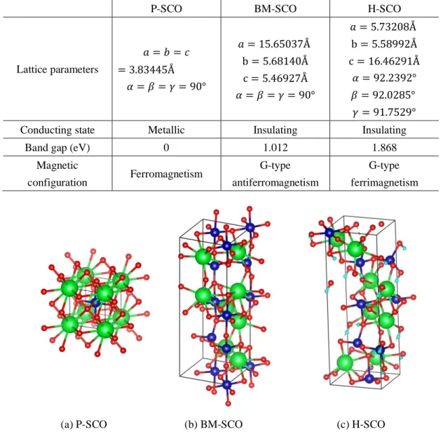
During the first step, high accuracy DFT calculations are conducted to relax crystal structures. After relaxations, the ground state atomic structures, lattice parameters, conducting states, band gaps, electronic density of states (DOS), and magnetic configurations of P-SCO, BM-SCO and H-SCO are determined and shown in Table 1 Fig. 2, and Fig. 3.
Table 1. Lattice parameters, conducting states, band gaps and magnetic configurations of SCO
P-SCO BM-SCO H-SCO
Lattice parameters 𝑎 = 𝑏 = 𝑐 = 3.83445Å 𝛼 = 𝛽 = 𝛾 = 90° 𝑎 = 15.65037Å b = 5.68140Å c = 5.46927Å 𝛼 = 𝛽 = 𝛾 = 90° 𝑎 = 5.73208Å b = 5.58992Å c = 16.46291Å 𝛼 = 92.2392° 𝛽 = 92.0285° 𝛾 = 91.7529°
Conducting state Metallic Insulating Insulating
Band gap (eV) 0 1.012 1.868
Magnetic configuration Ferromagnetism G-type antiferromagnetism G-type ferrimagnetism
(a) P-SCO (b) BM-SCO (c) H-SCO
Fig. 2. Atomic structures of SCO. The green, blue, red and cyan spheres denote Sr, Co, O and H atoms, respectively.
30
(a) P-SCO
SCOSCO
(b) BM-SCO
(c) H-SCO
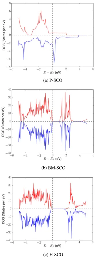
Fig. 3. Electronic density of states (DOS) of SCO as a function of electron energy. Red and blue lines represent spin up and spin down electronic DOS, respectively.
31
From Table 1 and Fig. 2, it can be seen that P-SCO is cubic with 𝑃𝑚3Ö𝑚 space group symmetry while BM-SCO is orthorhombic with 𝐼𝑚𝑎2 space group symmetry. Due to the existence of H atoms in H-SCO, the orthorhombic lattice of BM-SCO is slightly distorted and expanded around 8.27%, additionally its crystal space group symmetry reduces to the lowest 𝑃1. It should be noted that here we choose the 𝐼𝑚𝑎2 symmetry structure of BM-SCO as ground state structure according to the neutron powder-scattering experiment67
although some prior work shows contradictory ground state symmetries including 𝑃𝑚𝑐2768, 𝐼𝑚𝑎267,69, and 𝐼𝑚𝑚𝑎70.The lattice parameter of P-SCO is 3.83445Å, and
prior work finds 3.835Å71 and 3.842Å55. The lattice parameters of BM-SCO are found to
be 𝑎 = 15.65037Å , b = 5.68140Å, and c = 5.46927Å. The experimental results in BM-SCO are 𝑎 = 5.476Å , b = 15.769Å, c = 5.548Å71, 𝑎 = 5.65Å , b = 5.51Å, c =
15.76Å45, and finally 𝑎 = 15.6376Å , b = 5.5644Å, c = 5.4580Å which is obtained at
10K67; and the lattice parameters in these findings are consistent with ours given the
different definitions of lattice vectors. For H-SCO, the calculated lengths of lattice vectors are 𝑎 = 5.73208Å , b = 5.58992Å, c = 16.46291Å, while prior work has close values of 𝑎 = 5.79Å , b = 5.64Å , c = 16.64Å45, and 𝑎 = 5.726Å , b = 5.626Å , c =
16.066Å72.
The conducting state of SCO is determined from electronic DOS near the Fermi level. In Fig. 3, the electronic state near the Fermi level of P-SCO is non-zero and those of BM-SCO and H-BM-SCO are zero, so P-BM-SCO is metallic while BM-BM-SCO and H-BM-SCO are insulating. Besides, the band gap of H-SCO, ~1.868 eV (close to the DFT calculation of 1.99 eV72 but
smaller than the optical measurement of 2.84 eV45), is larger than BM-SCO’s band gap,
~1.012 eV (close to the DFT calculation of 1.37 eV72 and between the optical
measurements of 0.45 eV73 and 2.12 eV45), which implies larger electric resistivity in
H-SCO. In H-SCO, the spin up DOS is slightly different from the spin down DOS, indicating the spin degeneracy breaking and the non-zero net magnetization. These results are consistent with prior experiments and computations45,69,72.
The magnetic configurations of P-SCO, BM-SCO and H-SCO are ferromagnetic, G-type antiferromagnetic and G-G-type ferrimagnetic, respectively. These are the same as those reported previously45,46,55,67–73. In P-SCO, the magnetic moment of a Co atom is 2.114𝜇
9
and the magnetic moment of a formula unit is 2.626𝜇9. Prior work gives the magnetic moments of a Co atom and a formula unit as 2.2𝜇945, and 2.6𝜇
955 or 2.5𝜇946, respectively.
In BM-SCO, the magnetic moments of two types of Co atoms are 2.94𝜇9 and 2.89𝜇9,
while the total magnetic moment is 0. The neutron powder diffraction measurement gives the magnetic moments of 3.12𝜇9 and 2.88𝜇967, and the DFT calculation gives the value
around 3.1𝜇969. In H-SCO, the magnetic moments of two types of Co atoms reduce to
32
2.627𝜇972. H-SCOhasthe non-zero net magnetization and magnetic moments,even though
the magnetic ordering is still G-type antiferromagnetic. This arises from the unequal magnetic moments of two neighboring Co atoms with opposite spin orientations, which might be the effect of distorted oxygen octahedrons and tetrahedrons. According to prior work, H atoms just slightly perturbate antiferromagnetic exchange interactions locally69,
so the G-type antiferromagnetic ordering in BM-SCO is inherited into H-SCO and the overall magnetic configuration is thus G-type ferrimagnetic.
3.2. Phonon properties and thermal conductivities in SCO
3.2.1. Second-order and third-order force constants, net atomic charges and bond orders in P-SCO and BM-SCO
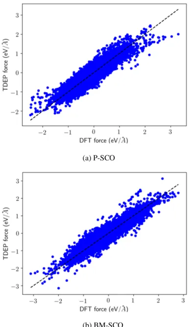
After obtaining the forces and displacements of P-SCO and BM-SCO at 300K from AIMD and recalculating them with pure DFT, TDEP is performed, and second- and third-order force constants are fitted using Eq. (2). The magnitudes of force constants versus interatomic distance, where interatomic distance is defined as the distance between the most distant atomic pairs for the third-order force constants, are plotted in Fig. 4. The comparison between the DFT and TDEP forces is shown in Fig. 5. The DFT and TDEP forces data points are generally around the dashed lines where the DFT and TDEP forces are equal, indicating good fitting results.
In Fig. 4, several features can be seen:
First, in P-SCO and BM-SCO, the largest force constant magnitudes are on site, which means distance among atoms is zero, or just within the first atomic shell, and with increasing distance, magnitudes of force constants decay very quickly, which means highly localized interatomic interactions. This is also observed in SrTiO38. Apart from on-site
force constant magnitudes, the largest force constant magnitudes appear at a distance around 1.9Å ~ 2.0Å, corresponding to Co - O pairs in both SCO. For on-site force constants, the largest magnitudes are among Co atoms. Similar phenomena occur in SrTiO3 where
the largest on-site and off-site force constant magnitudes are among Ti atoms and Ti - O pairs, respectively8.
Second, due to the lower symmetry in BM-SCO compared to that in P-SCO, atomic shells, appearing as discrete distances in Fig. 4, smear in BM-SCO, and this breaks some degeneracy in the force constants. Also, only on-site third-order force constants in P-SCO are absent due to the inversion symmetry in the cubic perovskite phase (since odd order terms change signs under the inversion operation), while a lack of inversion symmetry in BM-SCO preserves on-site terms.
33
Third, overall, force constant magnitudes in BM-SCO are larger than those in P-SCO, which indicates stronger interatomic interactions and anharmonicity in BM-SCO. This factor may be responsible for stronger phonon-phonon scattering, shorter phonon lifetimes, and lower thermal conductivity in BM-SCO. Given the fact mentioned above, that the largest force constant magnitudes are among on-site Co atoms and Co-O pairs, probably enhancement of magnitudes arises from Co atoms’ change. To unveil the details of this change, we perform the charge density partitioning and fitting in P-SCO and BM-SCO to determine net atomic charges and bond orders.
𝑛 = 2
𝑛 = 3
34 𝑛 = 2
𝑛 = 3
(b) BM-SCO
Fig. 4. Magnitudes of the second-order and third-order force constants of SCO as a function of interatomic distance. In the figures, 𝑛 indicates the order of force constants. For the third-order force constants, distance means the distance between the most distant atomic pairs.
35
By using the Chargemol program, the DDEC6 net atomic charges (hereafter, “NAC”) and bond orders (hereafter, “BO”) are computed as shown in Table 2. In P-SCO, Co atoms are surrounded by 6 O atoms and form octahedral CoO6; in BM-SCO, half of the Co atoms
are similar to those in P-SCO, while another half are surrounded by 4 O atoms and form tetrahedral CoO4. This kind of structural difference leads to different interatomic
interactions. In Table 2 it can be seen that when P-SCO transforms to BM-SCO, the average NAC of Co atoms decreases ~0.011𝑒 in CoO6, and increases ~0.055𝑒 in CoO4. Co atoms
in CoO4 have a little larger charge changes compared to those in CoO6; however, both of (a) P-SCO
(b) BM-SCO
Fig. 5. Comparison of DFT forces and TDEP forces. The dashed lines indicate the situations where DFT forces and TDEP forces are identical.
36
them have smaller charge changes compared to O atoms: the average NAC of O atoms increases ~0.191𝑒 in CoO6, and increases ~0.338𝑒 in CoO4. Tetrahedral CoO4 in
BM-SCO has more NAC of both Co and O atoms compared to octahedral CoO6 in BM-SCO
and P-SCO, and octahedral CoO6 in BM-SCO has opposite changes of Co and O atoms
compared to that in P-SCO. The larger changes of NAC in tetrahedral CoO4 are reasonable
because during transformation, oxygen vacancies are created in SCO and charge redistribution occurs locally.
Table 2. DDEC6 net atomic charges (NAC), distance between neighboring Co and O atoms (Co-O distance), ØdàÚ∙d§3Ø with 𝑛 = 2,3,4, DDEC6 bond orders between neighboring Co and O atoms (Co-O BO). Here Oct Co and Oct O denote Co and O atoms in octahedral CoO6, and Tet Co and Tet O denote Co and O atoms in tetrahedral CoO4. All values are averaged.
NAC (𝑒) Co-O distance (Å) Ødà∙d3 Ú3 Ø (𝑒4/Å4) Ø𝑒7𝑟∙ 𝑒< 4Ø (𝑒4/Å<) Ø𝑒7𝑟∙ 𝑒b 4Ø (𝑒4/Åb) Co-O BO P-SCO Oct Co 1.4275 - - - - - BM-SCO Oct Co 1.4169 - - - - - BM-SCO Tet Co 1.4824 - - - - - P-SCO Oct O -0.9759 1.9178 0.3788 0.1975 0.1030 0.4761 BM-SCO Oct O -1.1668 2.0569 0.3919 0.1917 0.0940 0.3967 BM-SCO Tet O -1.3143 1.8695 0.5573 0.2982 0.1597 0.6862
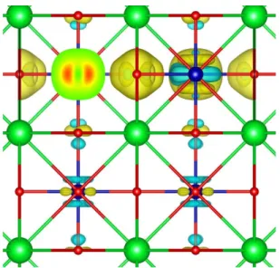
It can be seen in Fig. 6 that instantly after the creation of oxygen vacancies, the charge density around the Co atoms within CoO4 changes a lot, while the charge density around
the Co atoms within CoO6 changes slightly. Octahedral CoO6 doesn’t lose oxygen atoms,
so its local environment doesn’t change substantially; thus, NAC of Co and O change less. In contrast, tetrahedral CoO4 loses two oxygen atoms at first, so its local environment
changes dramatically. To balance this change, charge redistribution and transfer happen; as a result, NAC changes greatly. It can also be seen that the average distance between Co and O atoms in BM-SCO CoO4 is a little less than that in P-SCO CoO6, indicating a