Computational investigations of maximum flow algorithms

by

Ravindra K. Ahuja

Murali Kodialam

Ajay K. Mishra

James B. Orlin

WP #3811-95

April 1995

COMPUTATIONAL INVESTIGATIONS OF MAXIMUM FLOW

ALGORITHMS

Ravindra K. Ahuja, Murali Kodialam, Ajay K. Mishra, and James B. Orlin

ABSTRACT

The maximum flow algorithm is distinguished by the long line of successive contributions researchers have made in obtaining algorithms with incrementally better worst-case complexity. Some, but not all, of these theoretical improvements have produced improvements in practice. The purpose of this paper is to test some of the major algorithmic ideas developed in the recent years and to assess their utility on the empirical front. However, our study differs from previous studies in several ways. Whereas previous studies focus primarily on CPU time analysis, our analysis goes further and provides detailed insight into algorithmic behavior. It not only observes how algorithms behave but also tries to explain why algorithms behave that way. We have limited our study to the best previous maximum flow algorithms and some of the recent algorithms that are likely to be efficient in practice. Our study encompasses ten maximum flow algorithms and five classes of networks. The augmenting path algorithms tested by us include Dinic's algorithm, the shortest augmenting path algorithm, and the capacity scaling algorithm. The preflow-push algorithms tested by us include Karzanov's algorithm, three implementations of Goldberg-Tarjan algorithm, and three versions of Ahuja-Orlin-Tarjan excess-scaling algorithms. Among many findings, our study concludes that the preflow-push algorithms are substantially faster than other classes of algorithms, and the highest-label preflow-push algorithm is the fastest maximum flow algorithm for which the growth rate in the computational time is O(n1 5) on four out of five of our problem classes. Further, in contrast to the results of the worst-case analysis of maximum flow algorithms, our study finds that the time to perform relabel operations (or constructing the layered networks) takes at least as much computation time as that taken by augmentations and/or pushes.

1. INTRODUCTION

The maximum flow problem is one of the most fundamental problems in network optimization. Its intuitive appeal, mathematical simplicity, and wide applicability has made it a popular research topic among mathematicians, operations researchers and computer scientists.

The maximum flow problem arises in a wide variety of situations. It occurs directly in problems as diverse as the flow of commodities in pipeline networks, parallel machine scheduling, distributed computing on multi-processor computers, matrix rounding problems, baseball elimination problem, and the statistical security of data. The maximum flow problem also occurs as a subproblem while solving more complex problems such as the minimum cost flow problem and the generalized flow problem. The maximum flow problem also arises in combinatorics, with applications to network connectivity, and to matchings and coverings in bipartite networks. The book by Ahuja, Magnanti and Orlin [1993] describes these and other applications of the maximum flow problem.

Due to its wide applicability, designing efficient algorithms for the maximum flow problem has been a popular research topic. The maximum flow problem is distinguished by the long line of successive contributions researchers have made in obtaining algorithms with incrementally better worst-case complexity (see, e.g., Ahuja, Magnanti and Orlin [1993] for a survey of these contributions). Indeed, no other fundamental network optimization problem has witnessed as many incremental improvements in solution techniques as has the maximum flow problem. Some, but not all, of these theoretical improvements have produced improvements in practice. The purpose of this paper is to test some of the major algorithmic ideas developed in recent years and to assess their utility in practice.

Prior to the advent of preflow-push algorithms due to Goldberg and Tarjan [1986], Dinic's [1970] and Karzanov's [1974] algorithms were considered to be the fastest maximum flow algorithms. Subsequent developments from 1974 to 1986 included several algorithms with improved worst-case complexity, but these theoretical improvements did not translate into empirically faster algorithms. The novel concept of distance labels, in contrast to the layered (or, referent) network concept in Dinic's and Karzanov's algorithms, proposed by Goldberg and Tarjan [1986] led to breakthroughs both theoretically as well as empirically. Using distance labels in preflow-push algorithms, Goldberg and Tarjan [1986], and subsequently, Ahuja and Orlin [1989], Ahuja, Orlin and Tarjan [1989], Cheriyan and Hagerup [1989], and Alon [1990], obtained maximum flow algorithms with incrementally improved worst-case complexities. Some of these algorithms are also substantially faster than Dinic's and Karzanov's algorithms empirically, as the computational testings of Derigs and Meier [1989] and Anderson and Setubal [1992] revealed.

In this paper, we present the results of an extensive computational study of maximum flow algorithms. Our study differs from the previous computational studies in several ways. Whereas the previous studies focus primarily on CPU time analysis, our analysis goes farther and provides detailed insight into algorithmic behavior. It observes how algorithms behave and also tries to explain the behavior. We perform our empirical study using the representative operation counts, as presented in Ahuja and Orlin [1995], and Ahuja, Magnanti and Orlin [1993]. The use of representative operation counts allows us

(i) to identify bottleneck operations of an algorithm; (ii) to facilitate the determination of the growth rate of an algorithm; and (iii) to provide a fairer comparison of algorithms. This approach is one method of incorporating computation counts into an empirical analysis.

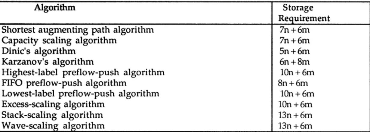
We have limited our study to the best previous maximum flow algorithms and some recent algorithms that are likely to be efficient in practice. Our study encompasses ten maximum flow algorithms whose discoverers and worst-case time bounds are given in Table 1.1. In the table, we denote by n, the number of nodes; by m, the number of arcs; and by U, the largest arc capacity in the network. For Dinic's and Karzanov's algorithm, we used the computer codes developed by Imai [1983], and for other algorithms we developed our own codes.

Table 1. 1 Worst-case bounds of algorithms investigated in our study.

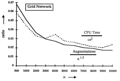
We tested these algorithms on a variety of networks. We carried out extensive testing using grid and layered networks, and also considered the DIMACS benchmark instances. We summarize in Tables 1.2 and 1.3 respectively the CPU times taken by the maximum flow algorithms to solve maximum flow problems on layered and grid networks. Figure 1.1 plots the CPU times of some selected algorithms applied to the grid networks. From this data and the additional experiments described in Sections 10 and 11, we can draw several conclusions, which are given below. These conclusions apply to problems obtained using all network generators, unless stated otherwise.

S.No. Algorithm Discoverer(s) Running Time

1. Dinic's algorithm Dinic [19701 O(n2m)

2. Karzanov's algorithm Karzanov [1974] O(n3)

3. Shortest augmenting

path algorithm Ahuja and Orlin [1991] O(n2m)

4. Capacity scaling algorithm Gabow [1985] and O(nm log U) Ahuja and Orlin [1991]

Preflow-push algorithms

5. Highest-label algorithm Goldberg and Tarjan [1986] O(n2ml/2)

6. FIFO algorithm Goldberg and Tarjan [19861 O(n3)

7. Lowest-label algorithm Goldberg and Tarjan [1986] O(n2m) Excess-scaling algorithms

8. Original excess-scaling Ahuja and Orlin [1989] O(nm + n2logU) n21 9. Stack-scaling algorithm Ahuja, Orlin and Tarjan [1989] Onm + log logU) 10. Wave-scaling algorithm Ahuja, Orlin and Tarjan [1989] O(nm + n2 )

n d Path Scaling Label Label Scaling Scaling Scaling 500 4 0.21 0.62 0.24 0.06 0.08 0.17 0.14 0.13 0.15 0.14 1000 4 0.67 2.05 0.72 0.15 0.20 0.52 0.36 0.31 0.37 0.40 2000 4 2.09 5.84 2.19 0.33 0.49 1.60 0.94 0.75 0.93 1.19 3000 4 3.96 11.52 4.14 0.50 0.80 3.23 1.59 1.21 1.63 2.36 4000 4 7.27 20.63 7.78 0.70 1.29 6.25 2.71 1.93 2.79 4.81 5000 4 13.00 52.97 13.80 0.90 2.67 12.78 5.91 3.70 6.50 9.84 6000 4 11.47 34.52 12.11 1.05 1.84 9.24 4.05 2.78 4.14 6.99 7000 4 15.45 41.26 16.37 1.30 2.44 13.20 5.26 3.61 5.43 9.67 8000 4 19.78 62.30 21.01 1.59 2.98 17.98 6.71 4.50 7.13 13.21 9000 4 26.77 78.22 28.47 1.77 4.16 25.67 9.08 5.87 10.06 18.55 10000 4 25.64 68.45 27.52 1.78 3.74 22.88 8.91 5.79 9.33 16.43 Mean 11.48 34.40 12.21 0.92 1.88 10.32 4.15 2.78 4.41 7.60 500 6 0.41 1.03 0.45 0.09 0.11 0.32 0.20 0.17 0.21 0.23 1000 6 1.20 3.12 1.27 0.19 0.26 0.95 0.49 0.39 0.48 0.58 2000 6 3.58 8.09 3.83 0.40 0.59 2.94 1.29 0.90 1.28 1.76 3000 6 6.46 13.78 6.86 0.61 0.92 5.22 2.19 1.42 2.03 3.00 4000 6 10.76 23.65 11.45 0.87 1.51 9.21 3.54 2.29 3.39 5.34 5000 6 13.78 26.71 14.93 1.06 1.66 11.33 4.38 2.68 4.19 6.45 6000 6 19.22 38.36 20.30 1.32 2.20 16.54 6.11 3.63 5.92 9.43 7000 6 27.22 57.09 29.30 1.56 3.16 25.09 8.86 5.09 9.03 14.76 8000 6 34.63 76.31 37.47 1.88 3.76 32.41 10.59 6.06 10.48 18.64 9000 6 29.04 47.88 31.14 1.74 2.93 22.76 8.43 4.96 7.51 12.01 10000 6 46.79 107.92 49.81 2.30 5.15 44.33 14.58 8.11 14.91 26.03 Mean 17.55 36.72 18.80 1.09 2.02 15.55 5.52 3.25 5.40 8.93 500 8 0.51 1.38 0.55 0.11 0.13 0.40 0.23 0.19 0.22 0.22 1000 8 1.46 3.45 1.59 0.22 0.29 1.14 0.56 0.42 0.53 0.61 2000 8 4.41 8.06 4.65 0.47 0.59 3.34 1.43 0.94 1.27 1.43 3000 8 8.63 16.22 9.13 0.74 0.97 6.69 2.55 1.58 2.27 3.05 4000 8 15.20 30.68 15.93 1.04 1.73 12.89 4.74 2.73 4.55 6.43 5000 8 23.68 56.43 25.09 1.46 3.19 21.47 7.27 4.21 7.52 11.82 6000 8 26.66 45.67 28.90 1.61 2.46 22.46 7.53 4.22 7.09 10.94 7000 8 41.92 83.05 45.42 2.02 4.22 38.63 12.76 6.66 12.98 20.60 8000 8 42.94 84.73 46.51 2.12 3.78 37.47 12.00 6.46 11.77 19.42 9000 8 55.32 108.73 59.83 2.57 5.46 50.98 16.03 8.44 16.39 27.47 10000 8 68.36 149.13 72.52 2.91 6.79 64.73 20.33 10.17 21.55 32.72 Mean 26.28 53.41 28.19 1.39 2.69 23.66 7.77 4.18 7.83 12.25 500 10 0.62 1.56 0.70 0.11 0.13 0.48 0.25 0.20 0.24 0.26 1000 10 1.71 3.59 1.93 0.26 0.30 1.35 0.59 0.44 0.54 0.58 2000 10 6.11 11.37 6.42 0.58 0.76 4.82 1.84 1.19 1.69 2.18 3000 10 10.34 16.75 11.57 0.84 1.07 8.17 2.94 1.78 2.57 3.62 4000 10 17.93 33.02 18.87 1.22 1.72 14.54 4.80 2.74 4.40 6.12 5000 10 23.56 43.23 25.85 1.47 1.94 18.79 6.03 3.34 5.39 7.97 6000 10 39.72 83.89 41.46 2.01 4.03 35.53 11.28 6.03 11.56 17.08 7000 10 44.22 75.38 47.23 2.16 3.30 36.54 11.55 5.88 10.68 16.41 8000 10 59.80 121.97 63.52 2.56 5.12 52.03 16.18 8.11 15.81 25.14 9000 10 64.85 118.98 69.94 2.72 4.70 54.64 17.49 8.47 16.81 24.73 10000 10 99.24 220.78 106.80 3.41 10.08 94.28 31.02 13.65 32.08 48.50 Mean 33.46 66.41 35.84 1.58 3.01 29.20 9.45 4.71 9.25 13.87

Table 1.3. CPU time (in seconds on Convex) taken by algorithms on the grid network.

I Grid Network I Shortest Augmenting Path

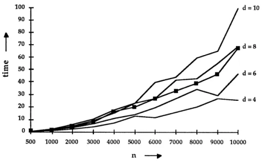
Dinic Lowest Label Karzanov Stack Scaling FIFO Highest Label 500 1000 2000 3000 4000 5000 6000 7000 8000 9000 10000 n N

Figure 1.1. CPU time (in seconds) taken by the algorithms on grid network.

Shortest PREFLOW-PUSH EXCESS SCALING

Aug. Capacity Dinic Highest FIFO Lowest Excess Stack Wave Karzanov

n d Path Scaling Label Label Scaling Scaling Scaling

500 5 0.41 1.71 0.39 0.11 0.15 0.27 0.21 0.21 0.23 0.33 1000 5 1.25 4.81 1.27 0.28 0.38 0.82 0.54 0.54 0.58 1.02 2000 5 3.84 15.17 3.97 0.76 1.12 2.62 1.54 1.47 1.68 3.18 3000 5 7.80 33.39 7.14 1.32 1.97 5.29 2.60 2.49 2.80 5.54 4000 5 15.89 74.02 13.82 1.98 3.14 11.67 4.50 4.01 4.93 12.37 5000 5 19.74 93.14 18.30 2.89 4.31 13.20 5.69 5.30 6.24 14.33 6000 5 26.80 110.53 24.61 3.65 5.80 21.31 7.86 7.29 8.72 20.05 7000 5 33.09 137.19 31.64 4.25 6.74 26.35 9.52 8.60 10.58 25.99 8000 5 39.07 167.13 40.24 4.88 8.11 30.13 11.36 10.26 12.82 31.61 9000 5 46.81 202.26 42.18 5.55 9.53 36.83 12.91 11.81 14.40 35.85 10000 5 67.48 283.88 57.37 6.94 11.43 52.41 16.40 14.85 18.24 51.58 Mean 23.83 102.11 21.90 2.96 4.79 18.26 6.65 6.07 7.38 18.35 70.00 0

jL

1. The preflow-push algorithms generally outperform the augmenting path algorithms and their relative performance improves as the problem size gets bigger.

2. Among the three implementations of the Goldberg-Tarjan preflow-push algorithms we tested, the highest-label preflow-push algorithm is the fastest. In other words, among these three algorithms, the highest-label preflow-push algorithm has the best worst-case complexity while simultaneously having the best empirical performance.

3. In the worst-case, the highest-label preflow-push algorithm requires O(n2 \Fm), but its empirical running time is 0(n1 5) on four of the five classes of problems that we tested.

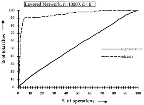
4. All the preflow-push algorithms have a set of two "representative operations": (i) performing pushes; and (ii) relabels of the nodes. We describe representative operations in Section 5 of this paper. See also Ahuja and Orlin [1995]. Though in the worst-case, performing the pushes is the bottleneck operation, we find that empirically this time is no greater than the relabel time. This observation suggests that the dynamic tree implementations of the preflow-push algorithms worsen the running time in the practice, though they improve the worst-case running time.

5. We find that the number of nonsaturating pushes is .8 to 6 times the number of saturating pushes.

6. The excess-scaling algorithms improve the worst-case complexity of the Goldberg-Tarjan preflow-push algorithms, but this does not lead to an improvement empirically. We observed that the three excess-scaling algorithms tested by us are somewhat slower than the highest-label preflow-push algorithm. We find the stack-scaling algorithm to be the fastest of the three excess-scaling algorithms, but it is on the average twice slower than the highest-label preflow-push algorithm.

7. The running times of Dinic's algorithm and the shortest augmenting path algorithm are comparable, which is consistent with the fact that both algorithms perform the same sequence of augmentations (see Ahuja and Orlin [1991]).

8. Though in the worst-case Dinic's algorithm and the successive shortest path algorithm perform O(nm) augmentations and take O(n2m) time, empirically we find that they perform no more than O(n1 6) augmentations and their running times are bounded by O(n2).

9. Dinic's and the successive shortest path algorithms have two representative operations: (i) performing augmentations whose worst-case complexity is O(n2m); and (ii) relabeling the nodes whose worst-case complexity is O(nm). We find that empirically the time to relabel the nodes grows faster than the time for augmentations. This explains why the capacity scaling algorithms (which decreases the worst-case running

time of augmentations at the expense of increasing the relabel time) do not improve the empirical running time over Dinic's algorithm.

2. NOTATION AND DEFINITIONS

We consider the maximum flow problem over a network G = (N, A) with N as the node set and A as the arc set. Let n = INI and m = IAI. The source s and the sink t are two distinguished nodes of the network. Let uij denote the capacity of each arc (i, j) E A. We assume that uij is integral and finite. Some of the algorithms tested by us (namely, the capacity scaling and excess scaling algorithms) require that capacities are integral while other algorithms don't. Let U = maxtuij: (i, j) E Al. We define the arc adjacency list A(i) of node i E N as the set of arcs directed out of node i, i.e., A(i) = {(i, k) E A: k E N).

A flow x is a function x : A --> R satisfying

xij - xji = O for all i E N - s, t, (2.1)

{j:(i,j)e A) {j:(j,i)E A}

x

xit = v, (2.2)

{i:(i,t) E A}

0 < xij < uij for all (i, j) E A, (2.3)

for some v > 0. The maximum flow problem is to determine a flow for which its value v is maximized.

A preflow x is a function x: A --> R satisfying (2.2), (2.3), and the following relaxation of (2.1):

E x j:(ij)i - 2 for all i E N - , . (2.4)

We say that a preflow x is maximum if its associated value v is maximum. The preflow-push algorithms considered in this paper maintain a preflow at each intermediate stage. For a given preflow x, we define for each node i E N - Is, t, its excess

e(i)= , j- x xji. (2.5)

j:(i,j)e A} j:(j,i)E A}

A node with positive excess is referred to as an active node. We use the convention that the source and sink nodes are never active. We define the residual capacity rij of any arc (i, j) E A with respect to the given preflow x as rij = (uij - xij) + xji. Notice that the residual capacity uij has two components: (i) (uij - xij), the unused capacity of arc (i, j), and (ii) the current flow xji on arc (j, i), which we can cancel to increase the flow from node i to node j. We refer to the network G(x) consisting of the arcs with positive residual capacities as the residual network.

A path is a sequence of distinct nodes (and arcs) i- i 2- ... -ir satisfying the property that for all 1 < p < r-l, either (i1, i2) e A or (i2, i1) E A. A directed path is an "oriented" version of the path in the sense that for any consecutive nodes ik and ik+1 in the walk, (ik, ik+₁) E A. An augmenting path is a directed path in which each arc has a positive residual capacity.

A cut is a partition of the node set N into two parts, S and S = N-S. Each cut [S, S] defines a set of arcs consisting of those arcs that have one endpoint in S and another in S. An s-t cut [S, S] is a cut satisfying the property that s E S and t E S Any (i, j) in [S, S] is a forward arc if i E S and j E S and is a backward arc if i S and

j

3. LITERATURE SURVEY

In this section, we present a brief survey of the theoretical and empirical developments of the maximum flow problem.

Theoretical Developments

The maximum flow problem was first studied by Ford and Fulkerson [1956], who developed the well-known labeling algorithm, which proceeds by sending flows along augmenting paths. The labeling algorithm runs in pseudo-polynomial time. Edmonds and Karp [19721 suggested two polynomial-time specializations of the labeling algorithm: the first algorithm augments flow along shortest augmenting paths and runs in O(nm2) time; the second algorithm augments flow along paths with maximum residual capacity and runs in O(m2logU) time. Independently, Dinic [19701 introduced the concept of shortest path

networks, called layered networks, and showed that by constructing blocking flows in layered networks, a

maximum flow can be obtained in O(n2_{m) time.}

Researchers have made several subsequent improvements in maximum flow algorithms by developing more efficient algorithms to establish blocking flows in layered networks. Karzanov [1974] introduced the concept of preflows and showed that an implementation that maintains preflows and pushes flows from nodes with excesses obtains a maximum flow in O(n3) time. Subsequently, Malhotra, Kumar and Maheshwari [1978] presented a conceptually simpler O(n3

) time algorithm. Cherkassky [1977] and Galil [1980] presented further improvements of Karzanov's algorithm that respectively run in O(n2_m1 / 2_{) and} o(n5/3m2 / 3) time.

The search for more efficient maximum flow algorithms led to the development of new data structures for implementing Dinic's algorithm. The first such data structure was suggested by Shiloach [1978], and Galil and Naamad [1980], and the resulting implementations ran in O(nm log2_{n) time. Sleator} and Tarjan [1983] improved this approach by using the dynamic tree data structure, which yielded an O(nm log n) time algorithm. All of these data structures are quite sophisticated and require substantial overheads, which limits their practical utility. Pursuing a different approach, Gabow [1985] incorporated scaling technique into Dinic's algorithm and developed an O(nm log U) algorithm.

A set of new maximum flow algorithms emerged with the development of distance labels by Goldberg and Tarjan [1986] in the context of preflow-push algorithms. Distance labels were easier to manipulate than layered networks and led to more efficient algorithms both theoretically and empirically. Goldberg and Tarjan suggested FIFO and highest label preflow-push algorithms, both of which ran in O(n3₎ time using simple data structures and in O(nm log(n2_{/m)) time using the dynamic tree data structures.} Cheriyan and Maheshwari [1989] subsequently showed that the highest-label preflow-push algorithm actually runs in O(n2,\m) time. Incorporating excess-scaling into the preflow-push algorithms, Ahuja and Orlin [1989] obtained an O(nm + n2log U) algorithm. Subsequently, Ahuja, Orlin and Tarjan [1989] developed two improved versions of the excess-scaling algorithms namely, (i) the stack-scaling algorithm with a time bound of O(nm + (n2log U)/(log log U)), and (ii) the wave-scaling algorithm with a time bound of O(nm + (n2log u)1/2). Cheriyan and Hagerup [1989], and Alon [1990] gave further improvements of these scaling algorithms. Goldfarb and Hao [1990 and 1991] describe polynomial time primal simplex algorithms that solves the maximum flow problem in O(n2m) time, and Goldberg, Grigoriadis, and Tarjan [1991] describe an O(nm log n) implementation of the first of these algorithms using the dynamic trees data structure.

Empirical Developments

We now summarize the results of the previous computational studies conducted by a number of researchers including Hamacher [1979], Cheung [1980], Glover, Klingman, Mote and Whitman [1983, 1984], Imai [1983], Goldfarb and Grigoriadis [1988], Derigs and Meier [19891, Anderson and Setubal [1992], Nguyen and Venkateswaran [1992], and Badics, Bodos and Cepek [1992].

Hamachar [1979] tested Karzanov's algorithm versus the labeling algorithm and found Karzanov's algorithm to be substantially superior to the labeling algorithm. Cheung [1980] conducted an extensive study of maximum flow algorithms including Dinic's, Karzanov's and several versions of the labeling algorithm including the maximum capacity augmentation algorithm. This study found Dinic's and Karzanov's algorithms to be the best algorithms, and the maximum capacity augmentation algorithm slower than both the depth-first and breadth-first labeling algorithms.

Imai [1983] performed another extensive study of the maximum flow algorithms and his results were consistent with those of Cheung [1980]. However, he found Karzanov's algorithm to be superior to Dinic's algorithm for most problem classes. Glover, Klingman, Mote and Whitman [1983, 1984] and Goldfarb and Grigoriadis [1988] have tested network simplex algorithms for the maximum flow problem.

Researchers have also tested implementations of Dinic's algorithm using sophisticated data structures. Imai [1983] tested Galil and Naamad's [1980] data structure, and Sleator and Tarjan [1983] tested their dynamic tree data structure. Both the studies observed that these data structures slowed down the original Dinic's algorithm by a constant factor. Until 1985, Dinic's and Karzanov's algorithms were widely considered to be the fastest algorithms for solving the maximum flow problem. For sparse graphs, Karzanov's algorithm was comparable to Dinic's algorithm, but for dense graphs, Karzanov's algorithm was faster than Dinic's algorithm.

We now discuss computational studies that tested more recently developed maximum flow algorithms. Derigs and Meier [1989] implemented several versions of Goldberg and Tarjan's algorithm. They found that Goldberg and Tarjan's algorithm (using stack or dequeue to select nodes for pushing flows) is substantially faster than Dinic's and Karzanov's algorithms. In a similar study, Anderson and Setubal [1992] find different versions (FIFO, highest label, stack, and highest label) to be best for different classes of networks and queue implementations to be about 4 times faster than Dinic's algorithm.

Nguyen and Venkateswaran [1992] report computational investigations with 10 variants of the preflow-push maximum flow algorithm. They find that FIFO and highest-label implementations together with periodic global updates have the best overall performance. Badics, Boros and Cepek [1992] compared Cheriyan and Hagerup's [1989] PLED (Prudent Linking and Excess Diminishing) algorithm and Goldberg-Tarjan's algorithm with and without dynamic trees. They found that Goldberg-Goldberg-Tarjan's algorithm outperformed PLED algorithm. Further, Goldberg-Tarjan's algorithm without dynamic trees was generally superior to the algorithm with dynamic trees; but they also identify a class of networks where the dynamic tree data structure does improve the algorithm performance.

In contrast to these studies, we find that our implementation of the highest-label preflow-push is consistently superior to all other implementations of the preflow-push algorithm on the five problem classes considered in our study. We find the highest-label preflow-push algorithm to be about 7 to 20 times faster than Dinic's algorithm and about 6 to 8 times faster than Karzanov's algorithm for large problem sizes. Our study also provides insights into these and several other algorithms not found in other computational studies.

4. NETWORK GENERATORS

The performance of an algorithm depends upon the topology of the networks it is tested on. An algorithm can perform very well on some networks and poorly on others. To meet our primary objective, we need to choose networks such that an algorithm's performance on it can give sufficient insight into its general behavior. In the maximum flow literature, no particular type of network has been favored for empirical analysis. Different researchers have used different type of network generators to conduct empirical analysis. We performed preliminary testing on four types of networks: (i) purely random networks (where arcs are added by randomly generating tail and head nodes; the source and sink nodes are also randomly selected); (ii) NETGEN networks (which are generated by using the well-known network generator NETGEN developed by Klingman et al. [1974]); (iii) random layered networks (where nodes are partitioned into layers of nodes and arcs are added from one layer to the next layer using a random process); and (iv) random grid networks (where nodes are arranged in a grid and each node is connected to its neighbor in the same and the next grid).

Our preliminary testing revealed that purely random networks and NETGEN networks were rather easy classes of networks for maximum flow algorithms. NETGEN networks were easy even when we generated multi-source and multi-sink maximum flow problems. For our computational testing, we wanted relatively harder problems to better assess the relative merits and demerits of the algorithms. Random

layered and random grid networks appear to meet our criteria and were used in our extensive testing. We give in Figure 4.2(a) an illustration of the random layered network, and in Figure 4.2(b) an illustration of the random grid network, both with width (W) = 3 and length (L) = 4. The topological structure of these networks is revealed in those figures. For a specific value of W and L, the networks have (WL + 2) nodes. A random grid network is from the parameters W and L; however, a random layered network has an additional parameter d, denoting the average outdegree of a node. To generate arcs emanating from a node in layer I in a random layered network, we first determine its outdegree by selecting a random integer, say w, from the uniform distribution in the range [1, 2d -1], and then generate w arcs emanating from node i whose head nodes are randomly selected from nodes in the layer (I + 1). For both the network types, we set the capacities of the source and sink arcs (i.e., arcs incident to the source and sink nodes) to a large number (which essentially amounts to creating w source nodes and w sink nodes). The capacities of other arcs are randomly selected from a uniform distribution in the range [500, 10000] if arcs have their endpoints in different layers, and in the range [200, 1000] if arcs have their endpoints in the same layer.

length .

I

'N

Figure 4.2 Example of a random layered network and a random grid network for width = 3 and length = 4.

k

In our experiments, we considered networks with different sizes. Two parameters determined the size of the networks: n (number of nodes), and d (average outdegree). For the same number of nodes, we tested different combinations of W (width) and L (length). We observed that various values of the ratio L/W gave similar results unless the network was sufficiently long (L >> W) or sufficiently wide (W >> L). We selected L/W = 2, and observed that the corresponding results were a good representative for a broader range of L/W. The values of n, we considered, varied from 500 to 10,000. Table 4.3 gives the specific values of n and the resulting combinations of W and L. For each n, we considered four densities d = 4, 6, 8 and 10 (for layered networks only). For each combination of n and d, we solved 20 different problems by changing the random number seeds.

Width (W) 16 22 32 39 45 50 55 59 64 67 71

Length(L) |31 45 63 77 89 100 109 119 125 134 141

n (approx.) 500 1,000 2,000 3,000 4,000 5,000 6,000 7,000 8,000 9,000 10,000 Table 4.3 Network Dimensions.

We performed an in-depth empirical analysis of the maximum flow algorithms on random layered and grid networks. But we also wanted to check whether our findings are valid for other classes of networks too. We tested our algorithms on three additional network generators: GL(Genrmf-Long), GW(Genrmf-Wide), and WLM(Washington-Line-Moderate). These networks were part of the DIMACS challenge workshop held in 1991 at Rutgers University. The details of these networks can be found in Badics, Boros and Cepek [19921.

5. REPRESENTATIVE OPERATION COUNTS

Most iterative algorithms for solving optimization problems repetitively perform some basic steps. We can decompose these basic steps into fundamental operations so that the algorithm executes each of these operations in 0(1) time. An algorithm typically performs a large number of fundamental operations. We refer to a subset of fundamental operations as a set of representative operations if for every possible problem instance, the sum of representative operations provides an upper bound (to within a multiplicative constant) on the sum of all fundamental operations performed by the algorithm. Ahuja and Orlin [1995] present a comprehensive discussion on representative operations and show that these representative operation counts can provide valuable information about an algorithm's behavior. We now present a brief introduction of representative operations counts. We will describe later in Section 8 the use of representative operations counts in the empirical analysis of algorithms.

Let an algorithm perform K fundamental operations denoted by a1, a2, ..., aK, each requiring 0(1) time to execute once. For a given instance I of the problem, let Cck(I), for k = 1 to K, denote the number of times

that the algorithm performs the k-th fundamental operation, and CPU(I) denote the CPU time taken by the algorithm. Let S denote a subset of {1, 2, ..., K). We call S a representative set of operations if CPU(I) = 0(k S ak(I)), for every instance I, and we call each c(k in this summation a representative operation count. In other words, the sum of the representative operation counts can estimate the empirical running time of an algorithm to within a constant factor, i.e., there exist constants c1 and c2 such that c1 ke Sak(I) < CPU(I) < c2 Xke Sak(I ) To identify a representative set of operations of an algorithm, we essentially need to identify a set S of operations so that each of these operations takes 0(1) time and each execution of every operation not in S can be "charged" to an execution of some operation in S.

6. DESCRIPTION OF AUGMENTING PATH ALGORITHMS

In this section, we describe the following augmenting path algorithms: the shortest augmenting path algorithm, Dinic's algorithm, and the capacity scaling algorithm. In Section 9, we will present the computational testings of these algorithms. In our presentation, we first present a brief description of the algorithm and identify the representative operation counts. We have tried to keep our algorithm description as brief as possible; further details about the algorithms can be found in the cited references, or in Ahuja, Magnanti and Orlin [1993]. We also outline the heuristics we incorporated to speed-up the algorithm performance. In general, we preferred implementing the algorithms in their "purest" forms, and so we incorporated heuristics only when they improved the performance of an algorithm substantially. Shortest Augmenting Path Algorithm

Augmenting path algorithms incrementally augment flow along paths from the source node to the sink node in the residual network. The shortest augmenting path algorithm always augments flow along a shortest path, i.e., one that contains the fewest number of arcs. A shortest augmenting path in the residual network can be determined by performing a breadth-first search of the network, requiring O(m) time. Edmonds and Karp [1972] showed that the shortest augmenting path algorithm would perform O(nm) augmentations. Consequently, the shortest augmenting path algorithm can be easily implemented in O(nm2₎ time. However, a shortest augmenting path can be discovered in an average of O(n) time. One method to achieve the average time of O(n) per path is to maintain "distance labels" and use these labels to identify a shortest path. A set of node label d(-) defined with respect to a given flow x are called distance labels if they satisfy the following conditions:

d(t) = 0, ( 6.1a)

d(i) < d(j) + 1 for every arc (i, j) in G(x). (6.lb)

We call an arc (i, j) in the residual network admissible if it satisfies d(i) = d(j) + 1, and inadmissible otherwise. We call a directed path P admissible if each arc in the path is admissible. The shortest

augmenting path algorithm proceeds by augmenting flows along admissible paths from the source node to the sink node. It obtains an admissible path by successively building it up from scratch. The algorithm maintains a partial admissible path (i.e., an admissible path from node s to some node i), and iteratively performs advance or retreat steps at the last node of the partial admissible path (called the tip). If the tip of the path, node i, has an admissible arc (i, j), then we perform an advance step and add arc (i, j) to the partial admissible path; otherwise we perform a retreat step and backtrack by one arc. We repeat these steps until the partial admissible path reaches the sink node, at which time we perform an augmentation. We repeat this process until the flow is maximum.

To begin with, the algorithm performs a backward breadth-first search of the residual network (starting with the sink node) to compute the "exact" distance labels. (The distance label d(i) is called exact if d(i) is the fewest number of arcs in the residual network from i to t. Equivalently, d(i) is exact if there is an admissible path from i to t. ) The algorithm starts with the partial admissible path P: = and tip i: = s, and repeatedly executes one of the following three steps:

advance(i). If there exists an admissible arc (i, j), then set pred(j): = i and P := Pu(i, j)). If j = t, then go to augment; else replace i by j and repeat advance(i).

retreat(i). Update d(i): = min{d(j) + 1: rij > 0 and (i, j) E A(i)}. (This operation is called a relabel operation.) If d(s) > n, then stop. If i = s, then go to advance(i); else delete (pred(i), i) from P, replace i by pred(i) and go to advance(i).

augment. Let A: = mintrij: (i, j) E P. Augment A units of flow along P. Set P : = , i := s, and go to advance(i).

The shortest augmenting path algorithm uses the following data structure to identify admissible arcs emanating from a node in the advance steps. Recall that for each node i, we maintain the arc adjacency list which contains the arcs emanating from node i. We can arrange arcs in these lists arbitrarily, but the order, once decided, remains unchanged throughout the algorithm. We further maintain with each node i an index, called current-arc, which is an arc in A(i) and is the next candidate for admissibility testing. Initially, the current-arc of node i is the first arc in A(i). Whenever the algorithm attempts to find an admissible arc emanating from node i, it tests whether the node's current arc is admissible. If not, it designates the next arc in the arc list as the current-arc. The algorithm repeats this process until it finds an admissible arc or reaches the end of the arc list. In the latter case, the algorithm relabels node i and sets its current-arc to the first arc in A(i).

We can show the following results about the shortest augmenting path algorithm: (i) the algorithm relabels any node at most n times; consequently, the total number of relabels is O(n2); (ii) the algorithm performs at most nm augmentations; and (iii) the running time of the algorithm is O(n2m).

The shortest augmenting path algorithm, as described, terminates when d(s) n. Empirical investigations revealed that this is not a satisfactory termination criterion because the algorithm spends too much time relabeling the nodes after the algorithm has already established a maximum flow. This happens because the algorithm does not know that it has found a maximum flow. We next suggest a technique that is capable of detecting the presence of a minimum cut and a maximum flow much before the label of node s satisfies d(s) > n. This technique was independently developed by Ahuja and Orlin [1991], and Derigs and Meier [1989].

To implement this technique, we maintain an n-dimensional array called number, whose indices vary from 0 to (n-l). The value number(k) stores the number of nodes whose distance label equals k. Initially, when the algorithm computes exact distance labels using breadth-first search, the positive entries in the array number are consecutive. Subsequently, whenever the algorithm increases the distance label of a node from k1 to k2, it subtracts 1 from number(k1), adds 1 to number(k2), and checks whether number(k1) = 0. If number(k1) = 0, then there is a "gap" in the number array and the algorithm terminates. To see why this termination criteria works, let S = {ie N: d(i) > k₁i and S= i E N: d(i) < k1i. It can be verified using the distance validity conditions (6.1) that all forward arcs in the s-t cut [S, S] must be saturated and backward arcs must be empty; consequently, [S, S] must be a minimum cut and the current flow maximum. We shall see later that this termination criteria typically reduces the running time of the shortest augmenting path algorithm by a factor between 10 and 30 in our tests.

We now determine the set of representative operations performed by the algorithm. At a fundamental level, the steps performed by the algorithm can be decomposed into scanning the arcs, each requiring (1) time. We therefore analyse the number of arcs scanned by various steps of the algorithm. Retreats. A retreat step at node i scans I A(i) I arcs to relabel node i. If node i is relabeled a(i) times, then the algorithm scan a total of i EN o(i) I A(i) I arcs during relabels. Thus arc scans during relabels, called arc-relabels, is the first representative operation. Observe that in the worst-case, each node i is relabeled at most n times, and the arc scans in the relabel operations could be as many as EiE N n A(i) I = n XiEN

I A(i) I = nm; however, on the average, the arc scans would be much less.

Augmentations. The fundamental operation in augmentation steps is the arcs scanned to update flows. Thus arc scans during augmentations, called arc-augmentations, is the second representative operation. Notice that in the worst-case, arcs-augmentations could be as many as n2m; however, the actual number would be much less in practice.

Advances. Each advance step traverses (or scans) one arc. Each arc scan in an advance step is one of the two types: (i) a scan which is later cancelled by a retreat operation; and (ii) a scan on which an augmentation is

subsequently performed. In the former case, this arc scan can be charged to the retreat step, and in the later case it can be charged to the augmentation step. Thus, the arc scans during advances can be accounted by the first and second representative operations, and we do not need to keep track of advances explicitly.

Finding admissible arcs. Finally, we consider the arcs scanned while identifying admissible arcs emanating from nodes. Consider any node i. Notice that when we have scanned I A(i) I arcs, we reach the end of the arc list and the node is relabeled, which requires scanning I A(i) I arcs. Thus, arcs scanned while finding admissible arcs can be charged to arc-relabels, which is the first representative operation.

Thus the preceding analysis concludes that one legitimate set of representative operations for the shortest augmenting path algorithm is the following: (i) arc-relabels; and (ii) arc-augmentations.

Dinic's Algorithm

Dinic's algorithm proceeds by constructing shortest path networks, called layered networks, and by establishing blocking flows in these networks. With respect to a given flow x, we construct the layered network V as follows. We determine the exact distance labels d in G(x). The layered network consists of those arcs (i, j) in G(x) which satisfy d(i) = d(j)+1. In the layered network, nodes are partitioned into layers of nodes V0, V1, V2, ..., Vl, where layer k contains the nodes whose distance labels equal k. Furthermore, each arc (i, j) in the layered network satisfies i E Vk and j E Vk_1 for some k. Dinic's algorithm augments flow along those paths P in the layered network for which i E Vk and j E Vk_1 for each arc (i, j) E P. In other words, Dinic's algorithm does not allow traversing the arcs of the layered network in the opposite direction. Each augmentation saturates at least one arc in the layered network, and after at most m augmentations the layered network contains no augmenting path. We call the flow at this stage a blocking flow.

Using a simplified version of the shortest augmenting path algorithm described earlier, the blocking flow in a layered network can be constructed in O(nm) time (see Tarjan [1983]). When a blocking flow has been constructed in the network, Dinic's algorithm recomputes the exact distance labels, forms a new layered network, and constructs a blocking flow in the new layered network. The algorithm repeats this process until obtaining a layered network for which the source is not connected to the sink, indicating the presence of a maximum flow. It is possible to show that every time Dinic's algorithm forms a new layered network, the distance label of the source node strictly increases. Consequently, Dinic's algorithm forms at most n layered networks and runs in O(n2m) time.

We point out that Dinic's algorithm is very similar to the shortest augmenting path algorithm. Indeed the shortest augmenting path algorithm can be viewed as Dinic's algorithm where in place of the layered network, distance labels are used to identify shortest augmenting paths. Ahuja and Orlin [1991] show that both the algorithms are equivalent in the sense that on the same problem they will perform the

same sequence of augmentations. Consequently, the operations performed by Dinic's algorithm are the same as those performed by the shortest augmenting path algorithm except that the arcs scanned during relabels will be replaced by the arc scanned while constructing layered networks. Hence, Dinic's algorithm has the following two representative operations: (i) arcs scanned while constructing layered networks; and (ii) arc-augmentations.

Capacity Scaling Algorithm

We now describe the capacity scaling algorithm for the maximum flow problem. This algorithm was originally suggested by Gabow [1985]. Ahuja and Orlin [19911 subsequently developed a variant of this approach which is better empirically. We therefore tested this variant in our computational study.

The essential idea behind the capacity scaling algorithm is to augment flow along a path with sufficiently large residual capacity so that the number of augmentations is sufficiently small. The capacity scaling algorithm uses a parameter A and with respect to a given flow x, defines the A-residual network as a subgraph of the residual network where the residual capacity of every arc is at least A. We denote the A-residual network by G(x, A). The capacity scaling algorithm works as follows:

algorithm capacity-scaling; begin

A: = 2 Llog ul; x2: = 0; while A > 1 do

begin

starting with the flow x = x2A, use the shortest augmenting path algorithm to construct augmentations of capacity A or greater until obtaining a flow xA such that there is no augmenting path of size A in G(x, A);

set x := xA;

reset A: = A/2;

end; end;

We call a phase of the capacity scaling algorithm during which A remains constant as the A-scaling phase. In the A-scaling phase, each augmentation carries at least A units of flow. The algorithm starts with A = 2Ll°g UJ and halves its value in every scaling phase until A = 1. Hence the algorithm performs 1 + Llog UJ = O(log U) scaling phases. Further, in the last scaling phase, A = 1 and hence G(x, A) = G(x). This establishes that the algorithm terminates with a maximum flow.

The efficiency of the capacity scaling algorithm depends upon the fact that it performs at most 2m augmentations per scaling phase (see Ahuja and Orlin [19911). Recall our earlier discussion that the shortest augmenting path algorithm takes O(n2m) time to perform augmentations (because it performs O(m) augmentations) and O(nm) time to perform the remaining operations. When we employ the shortest

augmenting path algorithm for reoptimization in a scaling phase, it performs only O(m) augmentations and, consequently, runs in O(nm) time. As there are O(log U) scaling phases, the overall running time of the capacity scaling algorithm is O(nm log U).

The capacity scaling algorithm has the following three representative operations:

Relabels. The first representative operation is arcs scanned while relabeling the nodes. In each scaling phase, the algorithm scans O(nm) arcs. Overall, the arc scanning could be as much as O(nm log U), but empirically it is much less.

Augmentations. The second representative operation is the arcs scanned during flow augmentations. As observed earlier, the worst-case bound on the arcs scanned during flow augmentations is O(nm log U).

Constructing A-residual networks. The algorithm constructs A-residual networks 1 + Llog UJ times and each such construction requires scanning O(m) arcs. Hence, constructing A-residual network requires scanning a total of O(m log U) arcs, which is the third representative operation.

It may be noted that compared to the shortest augmenting path algorithm, the capacity scaling algorithm reduces the arc-augmentations from O(n2_{m) to O(nm log U). Though this improves the overall} worst-case performance of the algorithm, it actually worsens the empirical performance, as discussed in Section 9.

7. DESCRIPTION OF PREFLOW-PUSH ALGORITHMS

In this section, we describe the following preflow-push algorithms: FIFO, highest-label, lowest-label, excess-scaling, stack-scaling, wave-scaling, and Karzanov's algorithm. Section 10 presents the results of the computational testing of these algorithms.

The preflow-push algorithms maintain a preflow, defined in Section 2, and proceed by examining active nodes, i.e., nodes with positive excess. The basic repetitive step in the algorithm is to select an active node and to attempt to send its excess closer to the sink. As sending flow on admissible arcs pushes the flow closer to the sink, the algorithm always pushes flow on admissible arcs. If the active node being examined has no admissible arc, then we increase its distance label to create at least one admissible arc. The algorithm terminates when there are no active nodes. The algorithmic description of the preflow-push algorithm is as follows:

algorithm preflow-push; begin

set x: = 0 and compute exact distance labels in G(x);

send xsj: = Us flow on each arc (s, j) E A and set d(s): = n;

while the network contains an active node do begin

select an active node i; push/relabel(i) end;

end;

procedure pushlrelabel(i); begin

if the network contains an admissible arc (i, j) then

push 8: = min e(i), rij) units of flow from node i to node j

else replace d(i) by minfd(j) + 1: (i, j) E A(i) and rij > 0};

end;

We say that a push of 8 units on an arc (i, j) is saturating if 8 = rij, and nonsaturating if 6 < rij. A nonsaturating push reduces the excess at node i to zero. We refer to the process of increasing the distance label of a node as a relabel operation. Goldberg and Tarjan [1986] established the following results for the preflow-push algorithm.

(i) Each node is relabeled at most 2n times and the total relabel time is O(nm).

(ii) The algorithm performs O(nm) saturating pushes.

(c) The algorithm performs O(n2m) nonsaturating pushes.

In each iteration, the preflow-push algorithm either performs a push, or relabels a node. The preflow-push algorithm identifies admissible arcs using the current-arc data structure also used in the shortest augmenting path algorithm. We observed in Section 6 that the effort spent in identifying admissible arcs can be charged to the arc-relabels. Therefore, the algorithm has the following two representative operations: (i) arc-relabels, and (ii) pushes. The first operation has a worst-case time bound of O(nm) and the second operation has a worst-case time bound of O(n2_m).

It may be noted that the representative operations of the generic preflow-push algorithm have a close resemblance with those of the shortest augmenting path algorithm and, hence, with those of Dinic's and capacity scaling algorithms. They both have arc-relabels as their first representative operation. Whereas the shortest augmenting path algorithm has arc-augmentation as its second representative operation, the preflow-push algorithm has pushes on arcs as its second representative operation. We note that sending flow on an augmenting path P may be viewed as a sequence of pushes along the arcs of P.

We next describe some implementation details of the preflow-push algorithms. All preflow-push algorithms tested by us incorporate these implementation details. In an iteration, the preflow-push algorithm selects a node, say i, and performs a saturating push, or a nonsaturating push, or relabels a node. If the algorithm performs a saturating push, then node i may still be active, but in the next iteration the algorithm may select another active node for push/relabel step. However, it is easy to incorporate the rule that whenever the algorithm selects an active node, it keeps pushing flow from that node until either its excess becomes zero or it is relabeled. Consequently, there may be several saturating pushes followed by either a nonsaturating push or a relabel operation. We associate this sequence of operation with a node examination. We shall henceforth assume that the preflow-push algorithms follow this rule.

The generic preflow-push algorithm terminates when all the excess is pushed to the sink or returns back to the source node. This termination criteria is not attractive in practice because this results in too many relabels and too many pushes, a major portion of which is done after the algorithm has already established a maximum flow. To speed up the algorithm, we need a method to identify the active nodes that become disconnected from the sink (i.e., have no augmenting paths to the sink) and avoid examining them. One method that has been implemented by several researchers is to occasionally perform a breadth-first search to recompute exact distance labels. This method also identifies nodes that become disconnected from the sink node. In our preliminary testing, we tried this method and several other methods. We found the following variant on the "number array" method to be the most efficient in practice.

Let the set DLIST(k) consist of all nodes with distance label equal to k. Let the index first(k) point to the first node in DLIST(k) if DLIST(k) is nonempty, and first(k) = 0 otherwise. We maintain the set DLIST(k) for each 1 < k < n in the form of a doubly linked list. We initialize these lists when initial distance labels are computed by the breadth-first search. Subsequently, we update these lists whenever a distance update takes place. Whenever the algorithm updates the distance label of a node from k1 to k2, we update DLIST(k1) and DLIST(k2) and check whether first(k1) = 0. If so, then all nodes in the sets DLIST(k1+1), DLIST(k1+2), ... have become disconnected from the sink. We scan the sets DLIST(k1+1), DLIST(kl+2), ..., and mark all the nodes in these sets so that they are never examined again. We then continue with the algorithm until there are no active nodes that are unmarked.

We also found another heuristic speedup to be effective in practice. At every iteration, we keep track of the number r of marked nodes. Wherever any node i is found to have d(i) > (n-r-1), we mark it too and increment r by one. It can be readily shown that such a node is disconnected from the sink node.

If we implement preflow-push algorithms with these speedups, then the algorithm terminates with a maximum preflow. It may not be a flow because some excess may reside at marked nodes. At this time, we initiate the second phase of the algorithm, in which we convert the maximum preflow into a

maximum flow by returning the excesses of all nodes back to the source. We perform a (forward) breadth-first search from the source to compute the initial distance labels d'(-), where the distance label d'(i) represents a lower bound on the length of the shortest path from node i to node s in the residual network. We then perform preflow-push operations on active nodes until there are no more active nodes. It can be shown that regardless of the order in which active nodes are examined, the second phase terminates in O(nm) time. We experimented with several rules for examining active nodes and found that the rule that always examines an active node with the highest distance label leads to minimum number of pushes in practice. We incorporated this rule into our algorithms.

An attractive feature of the generic preflow-push algorithm is its flexibility. By specifying different rules for selecting active nodes for the push/relabel operations, we can derive many different algorithms, each with different worst-case and empirical behaviors. We consider the following three implementations:

Highest-Label Preflow-Push Algorithm.

The highest-label preflow-push algorithm always pushes flow from an active node with the highest distance label. Let h* = max {d(i): i is active). The algorithm first examines nodes with distance label h and pushes flow to nodes with distance label h*-1, and these nodes, in turn, push flow to nodes with distance labels equal to h*-2, and so on, until either the algorithm relabels a node or it has exhausted all the active nodes. When it has relabeled a node, the algorithm repeats the same process. Goldberg and Tarjan [1986] obtained a bound of O(n3) on the number of nonsaturating pushes performed by the algorithm. Later, Cheriyan and Maheshwari [1989] showed that this algorithm actually performs O(n2m1 / 2) nonsaturating pushes and this bound is tight.

We next discuss how the algorithm selects an active node with the highest distance label without too much effort. We use the following data structure to accomplish this. We maintain the sets SLIST(k) =

ii:

for each 0 < k < 2n-1, points to the first node in SLIST(k) if SLIST(k) is nonempty, and is 0 otherwise. We define a variable level representing an upper bound on the highest value of k for which SLIST(k) is nonempty. In order to determine a node with the highest distance label, we examine the lists SLIST(level), SLIST(level-1), ..., until we find a nonempty list, say SLIST(p). We select any node in SLIST(p) for examination, and set level = p. Also, whenever the distance label of a node being examined increases, we reset level equal to the new distance label of the node. It can be shown that updating SLIST(k) and updating level is on average 0(1) steps per push and 0(1) steps per relabel. This result and the previous discussion implies that the highest-label preflow-push algorithm can be implemented in O(n2Nfm) time.

FIFO Preflow-Push Algorithm

The FIFO preflow-push algorithm examines active nodes in the first-in-first-out order. The algorithm maintains the set of active nodes in a queue called QUEUE. It selects a node i from the front of QUEUE for examination. The algorithm examines node i until it becomes inactive or it is relabeled. In the latter case, node i is added to the rear of QUEUE. The algorithm terminates when QUEUE becomes empty. Goldberg and Tarjan [1986] showed that the FIFO implementation performs O(n3) nonsaturating pushes and can be implemented in O(n3) time.

Lowest-Label Preflow-Push Algorithm.

The lowest-label preflow-push algorithm always pushes flow from an active node with the smallest distance label. We implement this algorithm in a manner similar to the highest-label preflow-push algorithm. This algorithm performs O(n2m) nonsaturating pushes and runs in O(n2m) time.

EXCESS-SCALING ALGORITHMS

Excess-scaling algorithms are special implementations of the generic preflow-push algorithms and incorporate scaling technique which dramatically improves the number of nonsaturating pushes in the worst-case. The essential idea in the (original) excess-scaling algorithm is to assure that each nonsaturating push carries "sufficiently large" flow so that the number of nonsaturating pushes is "sufficiently small". The algorithm defines the term "sufficiently large" and "sufficiently small" iteratively. Let emax = max(e(i): i active) and A be an upper bound on emax. We refer to a node i with e(i) > A/2 > emax/2 as a node with large excess, and a node with small excess otherwise. Initially A = 2 l°og UJ, i.e., the largest power of 2 less than or equal to U.

The (original) excess-scaling algorithm performs a number of scaling phases with different values of the scale factor A. In the A-scaling phase, the algorithm selects a node i with large excess, and among such nodes selects a node with the smallest distance label, and performs push/relabel(i) with the slight modification that during a push on arc (i, j), the algorithm pushes minte(i), rij, A-e(j)} units of flow. (It can be shown that the above rules ensure that each nonsaturating push carries at least A/2 units of flow and no excess exceeds A.) When there is no node with large excess, then the algorithm reduces A by a factor 2, and repeats the above process until A = 1, when the algorithm terminates. To implement this algorithm, we maintain the singly linked stacks SLIST(k) for each k = 1, 2,..., 2n-1, where SLIST(k) stores the set of large excess nodes with distance label equal to k. We determine a large excess node with the smallest distance label by maintaining a variable level and using a scheme similar to that for the highest-label preflow-push algorithm. Ahuja and Orlin [1989] have shown that the excess-scaling algorithm performs O(n2log U) nonsaturating pushes and can be implemented in O(nm + n2log U) time.

Similar to other preflow-push algorithms, the excess-scaling algorithm has (i) arc-relabels; and (ii) pushes, as its two representative operations. The excess-scaling algorithm also constructs the lists SLIST(k) at the beginning of each scaling phase, which takes 0(n) time, and this time can not be accounted in the two representative operations. Thus constructing these list, which takes a total of O(n log U) time, is the third representative operation in the excess-scaling algorithm.

We also included in our computational testing two variants of the excess-scaling algorithm with improved worst-case complexities, which were developed by Ahuja, Orlin and Tarjan [1989]. These are (i) the stack-scaling algorithm, and (ii) the wave-scaling algorithm.

Stack-Scaling Algorithm

The stack-scaling algorithm scales excesses by a factor of k > 2 (i.e., reduces the scale factor by a factor of k from one scaling phase to another), and always pushes flow from a large excess node with the highest distance label. The complexity argument of the excess-scaling algorithm and its variant rests on the facts that a nonsaturating push must carry at least A/k units of flow and no excess should exceed A. These two conditions are easy to satisfy when the push/relabel operation is performed at a large excess node with the smallest distance label (as in the excess-scaling algorithm), but difficult to satisfy when the push/relabel operation is performed at a large excess node with the largest distance label (as in the stack-scaling algorithm). To overcome this difficulty, the stack-stack-scaling algorithm performs a sequence of push and relabels using a stack S. Suppose we want to examine a large excess node i until either node i becomes a small excess node or node i is relabeled. Then we set S = i) and repeat the following steps until S is empty.

stack-push. Let v be the top node on S. Identify an admissible arc out of v. If there is no admissible arc, then relabel node v and pop (or, delete) v from S. Otherwise, let (v, w) be an admissible arc. There are two cases. Case 1. e(w) > A/2 and w X t. Push w onto S.

Case 2. e(w) <A/2 or w = t. Push min(e(v), rij, A-e(w)) units of flow on arc (v, w). If e(v) < A/2, then pop node v from S.

It can be shown that if we choose k = Flog U/log log U1, then the stack-scaling algorithm performs O(n2 log U/loglogU) nonsaturating pushes and runs in O(nm + n2 logU/log logU) time. The representative operations of this algorithm are the same as those for the excess-scaling algorithm.

Wave-Scaling algorithm

The wave-scaling algorithm scales excesses by a factor of 2 and uses a parameter L whose value is chosen appropriately. This algorithm differs from the excess-scaling algorithm as follows. At the

beginning of every scaling phase, the algorithm checks whether EiE N e(i) > nA/L (i.e., when the total excess residing at the nodes is sufficiently large). If yes, then the algorithm performs passes on active nodes. In each pass, the algorithm examines all active nodes in nondecreasing order of their distance labels and performs pushes at each such node until either its excess reduces to zero or the node is relabeled. We perform pushes at active nodes using the stack-push method described earlier. We terminate these passes when we find that ie N e(i) < nA/L. At this point, we apply the original excess-scaling algorithm, i.e., we push flow from a large excess node with the smallest distance label. If we choose L = rlog U, then the algorithm can be shown to perform O(n2iog U) nonsaturating pushes and to run in O(nm + n2 iogU) time.

KARZANOV'S ALGORITHM

Karzanov's algorithm is also a preflow-push algorithm, but pushes flow from the source to the sink using layered networks instead of distance labels. Karzanov [1974] describes a preflow-based algorithm to construct a blocking flow in a layered network in O(n2) time. The algorithm repeatedly performs two operations: push and balance. The push operation pushes the flow from an active node from one layer to nodes in the next layer (closer to the sink) in the layered network and the balance operation returns the flow that can't be sent to the next layer to the nodes in the previous layer it came from. Karzanov's algorithm repeatedly performs forward and reverse passes on active nodes. In a forward pass, the algorithm examines active nodes in the decreasing order of the layers they belong to and performs push operations. In a backward pass, the algorithm examines active nodes in the increasing order of the layer they belong to and performs balance operations. The algorithm terminates when there are no active nodes. Karzanov shows that this algorithm constructs a blocking flow in a layered network in O(n2_{) time; hence the overall running} time of the algorithm is O(n3).

The representative operations in Karzanov's algorithm are (i) the arc scans required to construct layered networks (which are generally m times the number of layered networks), and (ii) the push operations. The balance operations can be charged to the first representative operation. In the worst-case, the first representative operation takes O(nm) time and the second representative operation takes O(n3₎ time.

A Remark on the Similar Representative Operations for Maximum Flow Algorithms

The preceding description of the maximum flow algorithms and their analysis using representative operations yields the interesting conclusion that for each of the non-scaling maximum flow algorithms there is a set of two representative operations: (i) relabels; and (ii) either of augmentations and arc-pushes. Whereas the augmenting path algorithms perform the arc-augmentation, the preflow-push algorithms perform arc-pushes. The scaling based methods need to include one more representative operation corresponding to the operations performed at the beginning of a scaling phase. The similarity and