Computer modeling of a continuous manufacturing process

Computer Modeling of a Continuous Manufacturing Process by

Douglas Bohn

B.S., Chemical Engineering University of Minnesota, 1993

Submitted to the Department of Chemical Engineering And the Sloan School of Management

In Partial Fulfillment of the Requirements for the Degrees of Master of Science in Management

And

Master of Science in Chemical Engineering In conjunction with the

Leaders for Manufacturing Program At the

Massachusetts Institute of Technology June, 1998

C 1998 Massachusetts Institute of Technology All rights Reserved

Signature of the Author _

Department oi Chemical Engineering Sloan School of Management

May 8, 1998 Certified by

Professor Kevin Otto, Thesis Advisor Departmentof Mechanical Enineering Certified by_

Proiessor Steve Graves, Thesis Advisor Sloan School o~Management

Certified by

rrofefsor Charles C y, Thesis Reader DepartmentioPChe i lJ ngineering Accepted by_

Professor onu lunen

Departarst of ChemiqcljEnhneering Accepted by

Larry Aeln, Director oI iviaster's Program

Sloan School of Management

MASSACHUSETTS INSTITUTE OF TECHNOLOGY

JUN 2

5 1998

Science

Computer Modeling of a Continuous Manufacturing Process by

Douglas Bohn

Submitted to the MIT Sloan School of Management and the Department of Chemical Engineering on May 8, 1998 in partial fulfillment of the requirements for the degrees of

Master of Science in Chemical Engineering and Master of Science in Management

ABSTRACT

In this thesis, we develop process models for the dryer and the kiln processing units in the production of a refractory product. Working together, the plant and research center personnel were able to develop process models that accurately modeled the actual operating conditions. Applying sensitivity analysis to these models allowed us to understand the sources of variation

and reduce the variation by recommending process control changes, thereby eliminating the dryer/kiln as the bottleneck of the process. We used the computer models to predict the impact on final product quality of changes in the process inputs. In this process, quality is related to throughput: if quality requirements are not met, throughput rate needs to decrease. Thus, by

knowing the effect of the inputs on final product quality, we were able to determine the effects on throughput.

We used the computer models to run half factorial design of experiments (DOEs) in which the process inputs were varied. Then, we conducted a statistical analysis on the results.

These results determined which inputs have the largest impact on the processes and therefore should be controlled to minimize the variability of the outputs. The results of the model helped us develop recommendations around the following topics:

1. The tradeoff between air flow and air temperature: The models were used to determine the impacts that air flow and air temperature have on drying rates. In some cases, a higher air flow rate with a lower air temperature can lead to increased drying rates or vice versa.

2. The size of the equipment: Varying the size of the dryer/kiln will lead to changes in the residence time and thus will impact the drying and converting process. For instance, increasing the diameter of the equipment will lead to longer residence times and hence air temperature and flow rates will have a different effect than with a smaller diameter.

3. Process Control Parameters: Investigating the effect of several process control strategies led us to determine that we may be able to optimize the system further by changing our process control strategy. We used the models to determine how the process control strategy affects final product quality variability and throughput. Our initial results from the plant indicate that by following the recommendations

developed from the models, we can increase throughput rates, possibly by as much as 20%. This is a high enough throughput increase that the dryer/kiln is no longer the bottleneck. Furthermore, we changed the dimensions of some of the equipment and thus were able to change the

temperature and air flow patterns which may help reduce machine downtime. The models also suggest even further improvement through changes to the control strategy, though it is probably necessary to gain confidence in our ability to measure a different set of variables than are currently measured. Furthermore, the data from this measurement could be used to further validate the models.

Thesis Supervisors: Professor Steve Graves, Sloan School of Management

TABLE OF CONTENTS

1. PROJECT OVERVIEW 5

2. DRYER/KILN THEORETICAL BACKGROUND 14

3. DRYING THEORY 17

4. DESCRIPTION OF THE MODELS 22

5. MODEL VALIDATION 32

6. EFFECT OF AGGLOMERATE SIZE ON DRYING RATES 35

7. SENSITIVITY ANALYSIS 38

8. CONTROL STRATEGY 47

9. PLANT DRYING EXPERIMENTS 60

The author wishes to acknowledge the Leaders for Manufacturing Program for its support of this Work

The specific data given in this thesis has been altered to protect the confidential nature of the manufacturing processes studied. The conclusions and the methods used to obtain these conclusions are accurately described in

PROJECT OVERVIEW

The thesis will start out by giving the general background on the project, the product, and the manufacturing process. Then, a summary of the information from the literature on general drying theory will be given. Following the drying theory chapter, the actual computer models will be developed and validated. Next, the models will be used to determine the sensitivity of throughput and product quality to the process and

equipment inputs. Then, the models will be used to investigate the effects of several control strategies on throughput and product quality. Next, the plant implementation of the recommendations from the models will be discussed. Finally, the key learnings from the models will be summarized.

The output is a powder sold to other industrial companies and used mostly as an aid to their production process. The current demand for this product is high and one of the company's business objectives is to increase production without a significant capital expenditure. Developing process models could help the company not only increase throughput, but also develop a more complete understanding of the entire production process. Furthermore, by developing models, the company was able to capture the

learnings gained from this project and incorporate them into the models and thus was able to ensure that the company will be able to expand upon the knowledge gained during this project in the future.

The product is produced from a raw powdery material as purchased from an internal supplier. The main difference between the incoming powder and the outgoing product is the crystal size, which affects some of the physical properties. These physical properties are the main quality attributes of the final product. The chemical makeup of the

incoming raw material and the outgoing final product are identical. The Process Description section gives a generalized process overview.

The company currently manufactures the product at four plants; one in North America, two in Europe, and one in Asia. The current demand for the product is high and the forecast indicates that demand will remain high for the next few years. This has led to a capacity shortage in the industry, particularly in North America. The company believes that the capacity of the North America plant can be increased without undertaking a major capital project. Furthermore, there are several key operating differences that vary among each of the plants. Thus, process models were used to investigate the impact of each of the key operating inputs on throughput and product quality. Furthermore, the models

were used to understand the reasons for the production differences among plants around the world.

Problem Definition:

A more thorough understanding of the entire production process is desired with the ultimate goal of increasing production throughput. As will be discussed in the Process Description section, the production process is continuous with a break at the cooling bins. Therefore, output from one step directly affects the next step. In addition, outputs from certain steps are sent back to the preceding processing steps. For instance, the drying process uses the cooling bin and kiln exhaust air as process inputs. Thus, it is necessary to know how the entire system reacts to changes in inputs. A complete model that simulates the entire process is being developed. In addition to the processing steps affecting one another, the production schedule and logistics also affect the manner in which processing steps are carried out. Therefore a complete model which ties the

processing and the production steps together will help determine how the system's outputs are affected by the inputs. Also, the model will help determine how to optimize production given a certain level of demand.

In this thesis, we will develop process models for the dryer and the kiln processes. We will use the models to determine the sensitivity of the processes to variations in the process inputs. The dryer is the current bottleneck of the system and the kiln is the processing step at which the main quality attribute is determined. Therefore, each of these processing units is critical to the successful operation of the system. Moreover, as

discussed above the dryer and the kiln operations are interrelated to one another (the kiln outputs are used as inputs to the dryer). Therefore, modeling one without the other will not give an accurate representation of the "true" output. Once these process models are complete, the effect of inputs on the dryer/kiln systems outputs will be investigated. Process Description:

To gain an appreciation for the entire production process, this section will give a Figure 1.1: Simplified Process Flowsheet

Nucleator Agglomerate Former ) Dryer

Kiln Crush/Screener De-Ironer

Nucleator:

The raw material entering the process is initially ground to a fine powder in the nucleator processing step. Quality of the nucleator discharge is controlled by adjusting the feed rate to maintain the powder within certain pre-specified particle diameters. Producing fine particles requires a reduction in the feed rate, this reduces capacity.

Nucleator discharges that are too coarse result in reduced strength of the agglomerates produced in the agglomerate forming operation which leads to increased fines in the dryer and the kiln. (Excessive fines in the dryer and the kiln can significantly impact the firing conditions of the kiln which can have serious effects on the final product quality of the agglomerates).

Agglomerate Forming Step:

The powder is fed into this step and is distributed over the moving bed of forming agglomerates that have been previously wetted with a binder. The powder adheres to the wetted surface of the forming agglomerates. Agglomerates at the proper size leave the agglomerate former by passing through a screening system and enter the dryer. Keeping the agglomerate forming operations running smoothly is the key to a successful

agglomerate forming step. Variable binder addition or feed rates will lead to alternatively thick and thin layers of ground ore build up on the agglomerates. This may lead to weaker laminations and the agglomerate may actually fall apart upon further processing (this can lead to increased fines).

Drying Step:

The agglomerates enter the dryers within a certain moisture content range. The exhaust air from the kiln and the cooling bin are used as heat to the process. Ambient air

that is "bled" into the system controls the temperature. At high temperatures, heat transfer from the air to the agglomerates becomes so great, that the binder in the inner portion of the agglomerate begins to evaporate. When this happens, the inner vapor pressure can become so high that the agglomerate "explodes" (this phenomenon is termed

'popping'). The agglomerate popping leads to increased dryer fines. Occasional popping is acceptable and the resulting dryer fines are routed back to the agglomerate mill for recovery. The dried agglomerates then proceed onto the kiln.

Kiln:

The agglomerates entering the kiln should be completely dry. If they are not, popping will occur in the kiln. Typically, the agglomerates enter this step at a temperature of 400 F. Both methane and cooling air are fed into the kiln. The agglomerates enter at the top of the kiln and pass down the kiln while the air rises up. The agglomerates need to reach a specific minimum temperature for the product to reach the needed final product characteristics. If kiln temperatures reach the melting point of the material, the agglomerates will melt together. The melted together agglomerates are called "clinkers" and obviously have a negative impact on the kiln operations.

Furthermore, if the correct temperature range is not reached, the agglomerates can either be underfired or overfired in the kiln. To determine if the agglomerates are fired properly (i.e. if they have reached the proper degree of crystallinity), they are visually inspected and the agglomerate density is measured. If the population of agglomerates is underfired, the agglomerates are not being sufficiently heated and corrective action such as

decreasing the kiln pull rate or increasing gas flow rates should be taken. Conversely, if the population of over fired agglomerates is increasing then the kiln pull rates can be

increased or fuel rates reduced to reduce the heat treatment. The agglomerates exiting the kiln then enter the cooling bins where they are cooled down to approximately ambient conditions.

Crush/Screening:

The agglomerates exiting the cooling bin are fed into the crush/screening system. The agglomerates are initially fed into a primary crusher where initial size reduction takes place. Particles that meet the maximum size requirement are then passed through the screens. Those particles that are not yet small enough, pass through a roll crusher for further size reduction. The secondary crusher discharge is combined with the primary crusher discharge and are then transferred to the screening system. Thus, a closed loop is formed whereby oversize is continuously recycled till it is finally crushed to form the final product. The roll crusher gap is adjusted to control particle size distribution.

After crushing, the product needs to be de-ironed. A significant amount of iron from the crushers and other equipment often finds its way into the crushed product. The crushed product is fed past a magnetic belt. The magnetic cross belt removes the larger iron particles. For some products, additional de-ironing is needed. These products are directed to a more powerful de-ironer that removes the very fine iron filings.

Basics of the Dryer and the Kiln:

Since this project focused on the dryer/kiln system, a more detailed description of this system will be discussed.

Figure 1.2 shows a diagram of the dryer/kiln unit. As the figure indicates, wet agglomerates enter the top of the dryer and pass down through the dryer. After exiting the dryer, the agglomerates enter the kiln where they also pass down through the dryer.

Then, they pass into the cooling bin where they are cooled down to near ambient temperatures. The exiting hot air from the cooling bins, the table (at the bottom of the kiln), and the kiln stack gas is captured and is used as the heat source to the dryer. Ambient air is then bled in with the hot air to control the dryer temperature.

Figure 1.2:Process Flow of the Dryer/Kiln

W et Raw M ateridl Air HOT AIR HOT AIR FIRED MATERIAL

The significant process inputs and outputs to the dryer are shown in Figure 1.3. Figure 1.3

DRYER PROCESS INPUT 4

As can be seen from Figure 1.3, the dryer and the kiln units use as process inputs, the process outputs from each other: i.e. the dryer process outputs are the inputs to the

kiln and the kiln process outputs are used as inputs to the dryer. Thus the two units are linked together and must be studied together to determine the optimum operating conditions. The understanding of one process requires the understanding of the other.'

Before this project was undertaken, the opinions of how to increase

throughput varied. Some thought was given to increasing the drying capacity of the plant by expanding the heat and air capacity of the dryer. This would require a capital

expenditure. Another opinion was that by changing certain drying inputs, the drying capacity would increase. Furthermore, it was thought that most of the actual drying occurred in the dryer and that by changing conditions in the dryer, the drying rate could be increased. Finally, it was not known why the kiln could produce underfired

agglomerates and also fuse agglomerates together at what was thought to be the same process conditions. Through the use of the computer models, the plant and research personnel were able to answer these questions and gain new insights into the plant operations. The responses to variability in the inputs can be extremely complicated. Computer models that link the entire dryer/kiln system are the most effective method, and perhaps the only possible method, available to investigate the effect of the process inputs on the final process outputs.

Project Goals:

Our project goals are to develop an entire system of models that are linked together to give the us the ability to understand the effects on the product outputs from the inputs to the different operations in the chain of steps in the manufacturing process.

Throughout the thesis, the terms Process Input/Outputs will be used instead of the actual variable names. This was done to protect the confidentiality of the process.

Thus, we will be able to determine the effect of the processing inputs on both the dryer and the kiln system. In the next chapter of the thesis, we will provide a summary of the key calculations made involving the dryer and the kiln. Then, we will discuss the

background on drying theory. Next, we will develop and validate both the dryer and the kiln models. Once we validate the models, we will use them to perform a sensitivity analysis. Then, we will use the results of the sensitivity analysis to develop a control

strategy for the kiln. Finally, we give a summary of the key conclusions developed from the work.

DRYER/KILN THEORETICAL BACKGROUND

Before the models could be developed, we needed to gain a better understanding of the dryer and kiln's theoretical capabilities. This was a necessary first step to

determine if the development of computer models was needed. If these calculations indicated that there was not enough energy or air to further expand the capacity of the system, the development of the models would not have helped in increasing throughput. To complete the capability analysis, we calculated the overall energy balances, saturation

level of the dryer air, and the minimum amount of time needed to dry the material. Due to the confidential nature of the process, the specific air and heat capacity data are not given. This chapter will focus on the general calculations performed and the conclusions derived from these calculations.

Energy Balance Calculations:

The calculations indicated that over half of the energy input into the system is lost. The reasons for this energy loss include normal heat loss to the surroundings due to insufficient levels of insulation and open vents to the atmosphere. Thus, production throughput can be increased without increasing the energy capacity of the system. Drying Potential of the Cooling Bin Air:

The calculations also indicated that at typical throughput rates, 76% of the binder could be evaporated by using only the cooling bin air. Performing this calculation

provided a rough estimate of the amount of binder that could be evaporated using only the cooling bin air. The result from this calculation indicates that most of the binder can be driven off in the surge bin, but it is still difficult, or perhaps impossible, to decouple the kiln and the dryer since the dryer needs to have the energy provided to it by the kiln.

(Note: Some assumptions on the temperature and flow rate of the cooling bin air were made, but the values chosen are considered to be at least representative and the conclusion from these calculations is still considered valid.)

Air Saturation Level:

Initially, there was some thought that the binder may be condensing out in the dryer and causing the dryer to be the bottleneck operation. However, the calculations indicate that the saturation level of the air in the dryer is quite low (the relative humidity is less than 10%). Therefore, binder saturation levels in the dryer have little impact on the overall effectiveness of the dryer.

Minimum Drying Time:

Previously recorded data that plotted agglomerate moisture loss versus time for several different temperatures was used to calculate the minimum theoretical time to dry.

At temperatures above a certain point, agglomerate popping occurred during the experiment. This would indicate that energy transfer to the agglomerates was too high. (shown in Figure 2.1.)

The calculated rate of energy transfer to the agglomerates at the popping point was

Figure 2.1: Moisture

Loss

vs Time

0 10C 0 8C -2) 8 -C-Temp

I

assumed to be the maximum energy input to the agglomerates (this assumes that the heat transfer rate at the popping temperature was right at the edge of causing popping). Also, heat transfer to the agglomerates was assumed to be the rate limiting step at moisture levels greater than 8%. At less than 8% moisture content, heat conduction from outside of the agglomerates to inner moist core of the agglomerates was assumed to be the rate limiting step. Data from previous company experiments indicate that the drying rate is

linear at moisture levels greater than 8% and becomes non-linear at moisture levels below 8%. Using the previous data, time to go from 8% moisture to 0% moisture was estimated to be about 30 minutes. Then using the maximum heat transfer rate to the agglomerates, the calculations indicated that the time to decrease the moisture content from 20% to 8% is about 20 minutes. Thus, the minimum theoretical drying time is about 50 minutes. The actual dryer residence times are much greater than 50 minutes and thus the agglomerate spends enough time in the dryer.

Our conclusions from the above analysis are that the system has enough energy, air, and residence time to dry the agglomerates. The main problems are energy loss, and variable drying rates. Actual plant data indicate that product from one side of the dryer has different moisture contents than those from the other side even though, the incoming moistures were approximately equal. In one case, the moisture contents of the

agglomerate taken from one side of the dryer differed by 15% from those taken on the other side. This data verify that variable drying rates are a major roadblock to increasing dryer throughput rates.

The next chapter will discuss the theory of drying. This will lay the groundwork for the discussion of the actual model development that will be given in Chapter 4.

DRYING THEORY

To develop the dryer model, we needed to gain an understanding of the drying process. By using the references given at the end of the chapter, we developed equations that are used in the dryer model. Not only did understanding drying theory help us

develop the computer models, but it also helped us gain a level understanding necessary to troubleshoot the dryer on a daily operating basis.

The drying model specified two different regions of drying. The first is the heat transferred controlled region, and the second is the heat conduction controlled region. Heat Transferred Controlled Region:

In the heat transferred controlled region, which occurs at moistures greater than 8%, the amount of heat transfer from the air to the agglomerates controls the drying rate. The binder is evaporated by the energy that is transferred from the air to the agglomerates. Equation 3.1 calculates the amount of heat transferred from the air to the agglomerates.

(3.1) Q = h*Ab*(Ta-Tb)

where:

h = heat transfer coefficient (J/S*K*m2)

Ab = Effective surface area of the agglomerates (m2) Tb = Temperature of the agglomerates (K)

Ta = Temperature of the air (K)

Q = Heat transferred to the agglomerates (J/s) The equation for h is2:

(3.1A) h = [(k/cpf*i)2/3]*[2.876/Nre + 0.3023/Nre3]*cp*v'*p/E where:

Nre=Dp*G'/g

Nre=Reynolds number

G= superficial mass velocity (kg/s)

E= Void fraction

v'= Superficial velocity of the gas Cpf=Heat capacity of the air

Cp = Heat capacity of the agglomerates p = Density of the agglomerates

g= Viscosity of the air

k=Thermal conductivity of the air.

(Note: The original form of Equation 3.1A has the Reynolds number raised to the 0.35 power but bench scale drying experiments had a better fit with a 0.3 coefficient. 2)

Then, Equation 3.2 calculates the evaporation rate.

(3.2) E = Q/(Hvap)

where:

Hvap = Heat of vaporization of the binder

The energy is transferred to the agglomerates at a constant rate (assuming the air temperature is constant), and therefore the drying rate is uniform across the agglomerate surface and throughout time during the heat transfer controlled region. As the binder evaporates, the surface of the agglomerates becomes dry and the heat conduction controlled drying region begins which results in decreasing the drying rate. Heat Conduction Controlled Region:

In this region, the heat that is transferred to the agglomerates needs to conduct through the agglomerates to be able to evaporate the binder that is in the center of the agglomerates. Then, the binder vapor is transferred through the agglomerate channels and exits the agglomerate. The steps to drying in this region are:

1. Heat transferred from the air to the agglomerates

2. Heat conducted from the surface of the agglomerates to the moist center 3. Binder is evaporated

4. Binder vapor diffuses through the channels of the agglomerate to the outer surface

Of the steps listed above, the rate limiting step is Step #2. As mentioned earlier, previous company experiments indicated that the drying curves become non-linear at about 8% moisture content. This indicates that the drying mechanism converts from the heat transferred controlled region to the heat conduction controlled region at 8% moisture.

Equation 3.3 gives the heat conduction rate for spherical shapes in the heat conduction controlled drying region.3

(3.3) Q/Qc = 1- Cq*exp(-E*Fo) where:

Q = heat conduction rate

Qc = reference enthalpy of the material

Cq= Constant which depends upon the heat transfer coefficient (h), the heat conductivity (k) of the spheres, and the temperature difference between the air and the agglomerates (AT)

E = Constant that depends on h, k, and AT

Fo = Fourier number = a*t/R2 _{(a = thermal diffusivity of the agglomerate,}

t = time of drying, and R = Effective agglomerate radius) Since the amount of heat conducting to the center of the agglomerate is proportional to the amount of drying in the center of the agglomerate, the amount of moisture in the agglomerate can be substituted for the heat conduction rate:

(3.4) Mt/M0 = 1 -A*exp(-B*t/R2)

where:

Mt = drying rate (kg of binder/minute)

Mo = Initial amount of binder in the agglomerate A = constant which depends on Cq

B = constant which depends on E and a t = time of drying

R = Effective radius of the agglomerate

Note that another logical approach to drying would assume the following drying steps: 1. Mass diffusion of the binder in the center of the agglomerates to the outside

2. Heat transfer from the air to the agglomerates

3. Evaporation of the binder vapor at the surface of the agglomerates

In this drying mechanism, mass diffusion (Step 1) is the rate limiting step. The equation governing Step One in a spherical shape is :

(3.5) Mt/M0 = 1 - C*exp(-D*t/R2)

This is identical to the equations developed in the heat conduction case. The only difference is that the constants C and D should not depend on temperature. Since the

regression indicated a slight dependence on temperature (a regression indicated that the t-ratio for the temperature coefficient is 3.90), the heat conduction mechanism is probably correct. However, the form of the equation is the same; the regressions will give similar results and the equations to be used in the model to simulate drying in this region will be identical. Thus the difference between heat conduction controlled vs. mass diffusion controlled is not important.

In this chapter, we summarized the fundamental theory of drying and how it applies to the drying of the agglomerates. There are two regions to drying: the heat transferred controlled region and the conduction/diffusion controlled region. In the heat transferred control region, drying is controlled by the temperature difference between the air and the agglomerate and by the value of the heat transfer coefficient. Equations 3.1 and 3.1 a give the necessary relationships. In the conduction/diffusion controlled region, the size of the agglomerate and the heat transfer properties (the material conductivity, heat transfer coefficient from the air to the agglomerates, and the thermal diffusivity) control the drying rate. In the next chapter, we will use these equations to develop a

model that will predict the drying rate of the agglomerates under different drying conditions. We will also develop the kiln model in the next chapter.

REFERENCES FOR THIS SECTION:

1. Crank, The Mathematics of Diffusion, Oxford Science Publications, 1979, pp 96-97

2. Geankoplis, Transport Processes and Unit Operations, Allyn and Bacon, 1983, pp 244-250 and pp

544-554

DESCRIPTION OF THE MODELS

Now that we have presented the theory behind the drying model, we develop both the dryer and kiln models. We will focus on the basic algorithm used in the codes and will further discuss the equations used. In the next chapter, we will validate the models developed in this chapter. Then, we will use the models to determine the effect of the processing inputs on throughput and product quality.

The models for the dryer and kiln code are finite element based models. The models slice up the dryer and kiln along the material flow path into many sections or nodes. Heat transfer equations and energy balance equations within each slice calculate the temperature of the agglomerate and the air in each node. The dryer code also

calculates the amount of moisture in the agglomerates within each node. The framework of the codes will be discussed below.

Dryer Code Assumptions:

* All agglomerates are assumed to be of equal temperature within a node and there is assumed to be no temperature distribution in the agglomerate. * The air that enters the dryer goes straight up the dryer. The cross section

within the dryer is cut into three equal areas. The percent air entering each of these three areas is an input to the model.

* The air within the surge bin is assumed to be equally distributed.

* At moisture levels greater than 8%, the agglomerates are in the heat transfer controlled region. With less than 8% moisture, the agglomerates are in the

Dryer Model:

The dryer model is a finite element model that solves the energy balance at each slice. The model calculates the amount of energy transferred to and from the

agglomerates at each node. Then, the model uses the amount of energy being transferred to calculate the amount of binder that is evaporated and the temperature of the air and the agglomerates. The inputs to the model are:

1. Stack gas temperature (Stack gas is the air leaving the kiln and entering the dryer)

2. Stack gas flow rates entering the dryer

3. Percent of ambient air that enters the dryers. (This along with the stack gas temperature controls the dryer inlet air temperature and the dryer inlet flow rate)

4. Percent air distribution across the three radial nodes in the dryer.

5. Throughput rate of the agglomerates in the dryer. 6. Length of the surge bin

7. Temperature of the air entering the surge bin. 8. Flow rate of the air entering the surge bin. 9. Radius of the agglomerates entering the dryer

10. Incoming moisture of the agglomerates. The outputs of the models are

1. Moisture profile of the agglomerates within the surge bin and the dryer.

2. Temperature profile of the air and agglomerates within the surge bin and the dryer.

(Note: Both the temperature and moisture profile include the agglomerate exiting temperature and moisture.)

As discussed in the drying theory section, agglomerate drying occurs in two regions; the heat transfer controlled region and the heat conduction controlled region. The model made several assumptions during each drying region.

1. Agglomerate temperature less than 100 C; in this region, all of the energy that was transferred to the agglomerate was used to heat the

agglomerate and the binder up to 100 C.

2. Agglomerate temperature @ 100 C; in this region, all of the energy transferred to the agglomerate was used to evaporate the binder. (Drying in this region is assumed to be controlled by the heat transfer controlled and the heat conduction controlled mechanism as discussed in the above section.)

3. Agglomerate moisture @ 0%: all of the energy is used to heat the agglomerate.

In regions 1 and 3, the model assumed that the temperature of the agglomerate was uniform. In other words, as heat is transferred to the agglomerate, it is uniformly spread out throughout the agglomerate to keep the temperature profile uniform. Also, the model assumed that no binder is evaporating in Region 1. This is probably not exactly true, since as the temperature increases the binder vapor pressure increases which would increase the evaporation rate. Finally, the model assumed that in Region 2 the drying

mechanism converts from the heat transfer controlled region to the heat conduction controlled region at 8% moisture. As mentioned previously, an earlier company report indicates that the drying rate is relatively constant from 20% moisture to 8% moisture. After 8% moisture, the drying rate is no longer constant.

Drying Model Equations:

To verify Equation 3.5, actual agglomerate drying experiment data, similar to that given in Figure 2.1, was regressed against Equation 3.5. The method described below transformed the data so that it could be regressed against Equation 3.5.

(4.1) D=Mt/Minf-Mto/Minf where:

Mt= moisture content at time t

Mto= moisture content at the beginning of the heat conduction controlled region = 0.08

Minf = moisture content of the agglomerates before drying begins

D = parameter that characterizes the percent drying from the start of the heat conduction controlled region

Then, rearranging Equation 3.4 to indicate that drying has already taken place in the heat transfer controlled region, gives:

(4.2) 1-Mt/Mint+Mto/Minf=A*exp(B*t/R2)= 1-D

Where A, B, and D are parameters that, if Equation 3.5 is valid, will statistically fit to the data from the agglomerate drying experiments.

Taking the natural log of both sides of Equation 4.2 gives:

(4.3) ln(1-Mt/Minf-Mto/Minf)= In(A) + B*t/R2 = In(1-D)

Thus a plot of In(1-Mt/Minf-Mto/Minf) vs t should give a straight line. Figure 4.1 plots In(1-Mt/Minf-Mto/Minf) vs t for four different temperatures. As can seen from Figure 4.1,

the correlation coefficients are above 0.97 which verifies that Equation 3.5 will give good results.

Since the variables B and A should be temperature dependent, a regression of ln(1-Mt/Mmf-Mto/Minf) vs. time and temperature should show a temperature dependence. This regression is shown in Figure 4.2. The equation of the regression is:

(4.4) Mt=Minf*[1-exp(-Po+Pl(t-to)+ 2*Temp)]+Mto

Where, the

3

Equation 4.4 was used to model the drying rate in the heat conduction controlled region. The temperature and the time terms in Equation 4.4 are also dependent upon the agglomerate radius. Thus, Equation 4.5 gives the final form of the equation.

FIGURE 4.2

Actual vs Predicted In(1-M/MinfMto/Minf)

0.25 0.2 0.15 0.1 0.05 0 0.05 0.1 0.15 0.25 Predicted In(1-M/Mn,-M Mnf)₁

Assumptions of the Kiln Code: The model:

* assumed no temperature distribution within the agglomerate.

* Assumed that all agglomerates within a node to be of equal temperature. The more nodes that are used, the better this assumption becomes. However, the

model indicates that the temperature profile does not vary that much with 1000 vs 10 nodes. Thus, we used 10 nodes for most of the analysis since this significantly reduced computation time.

* calculated heat loss through the kiln shell by summing the heat resistance in a series. The model used the following equation to determine the heat losses.

Ql=Ka*Ac*(T-Tamb) where: QI = energy losses

Ka = 1/h + k/dx + 1/h

y = 1.0011x F = 0.921

(h=heat transfer coefficient from the air to the walls, dx = kiln shell thickness, k=heat conductivity coefficient of the refractory) * assumed that radiation from the agglomerates occurs node to node.

Agglomerates within a node do not radiate to one another. This becomes a better assumption as node size decreases. As discussed above the temperature profile varied only a small amount from 1000 to 10 nodes, which would indicate that this is a good assumption.

* assumed that all of the air went straight up the kiln. If the air is properly distributed this should occur. Measurement of the air flow rates leaving the kiln at the top and those entering the kiln indicate that the air must be going up, therefore this is probably a pretty good assumption.

Kiln Model Inputs:

1. Agglomerate throughput rate 2. The ratio of combustion air to gas.

3. Incoming radius of the agglomerates. 4. Incoming temperature of the agglomerates.

5. Gas flow rate 6. Height of the kiln

7. Lower and upper cooling air flow rates. 8. Radius of the kiln

9. Location of the burner (gas inlet location) 10. Location of the cooling air inlets to the dryer.

The outputs of the models are the air and agglomerate temperature distribution within the kiln and the outgoing final quality of the agglomerates.

The kiln model is an explicit finite element model that solves an energy balance for the agglomerates and the air at each node. The model's first step is the initialization of the agglomerate and air temperatures. The model chooses the initial temperatures such

that the air and agglomerate temperatures are identical at each node. After the model completes the initialization, it computes the energy that is added to the agglomerate and the air at each slice.

The model computes the heat transferred from the air to the agglomerates by using Equation 4.6:

(4.6) E= h*Ab*(Ta-Tb)

where:

E = Energy transferred to the air

h = heat transfer coefficient from air to the agglomerates

Ab = effective surface area of the agglomerates assumed to be 122.25*(effective agglomerate radius/.55)/cubic meter of the node volume (at 75 % of the actual surface area and at 0.55 inches, the effective surface area of the agglomerates is 122.25/cubic meter

Tb = Temperature of the agglomerates in the given nodes Ta = Temperature of the air in the given nodes.

Next, the model computes the heat transferred to the agglomerates via radiation using Equation 4.7:

(4.7) E=E*Y*Ac*(TI4-T24)

where;

E = energy transferred via radiation S= emissivity of material

a = radiation coefficient (5.67*10- 7 J/m2*K4)

Ac = agglomerate contact surface area between nodes T1= Agglomerate temperature in the node being considered

T2= Agglomerate temperature in the node either above or below that being

considered.

Next, Equation 4.8 calculates the energy transferred due to material movement. (4.8) E = m*Cp*(TI-T2)

where:

E = Energy transferred to the node from movement of the agglomerates or the air. m = Mass flow rate of the agglomerates or the air

dt = time step (equal to .000035 seconds)

Cp = Heat capacity of the agglomerates or the air

T1= Temperature of the air or the agglomerates in the node that the agglomerates

or the air are flowing from.

T2 = Temperature of the air or the agglomerates in the node that the air and the agglomerates are flowing into.

(Note: Where the cooling air is entering the kiln and T1 is assumed to be equal to the

ambient air temperature.)

Then, the model calculates the energy input from the combustion of the gas by multiplying the gas flow rate with the heat of combustion of methane. This energy is only added to the node where the gas is entering.

Next, all of the energy inputs are added up for the agglomerate and the air at each node. Then, Equation 4.9 calculates the new temperature at each node.

(4.9) Tnew = Told + dt*Etot/(m*Cp)

where:

Tnew = The new temperature at the node

Told = The previous or the old temperature at each node dt = The time step (set at 0.000035 seconds)

Etot = Summation of the above calculated energies

m = mass of either the air or the agglomerates in each node Cp = Heat capacity of either the air or the agglomerates.

The model repeats each of these calculations until Tnew and Told in Equation 4.9 converge.

Now that we have developed the models, we will validate the models versus actual plant data in the next chapter. Once we have validated the models, we will use them in Chapters 6 through 8 to learn about the manufacturing system.

MODEL VALIDATION

Our next step in this project was to validate the models that were developed in the previous chapter. The validation process enabled us to improve the models and gave us the confidence that the model output was correct and could be used for process

improvement recommendations.

Rigorously validating the models was difficult because most of the inputs and outputs of the models are either not measured at all or not measured on a regular basis (this is part of the motivation for building the models). Hence, completely validating the model versus actual plant operating data was not feasible. However, the model could be related to variables that are routinely measured, and thus could be indirectly validated. For example, one of the kiln model outputs is measured regularly, and the recorded data

verify the model results. Also, anecdotal evidence suggests that the models adequately describe the actual behavior.

Dryer verification:

The data collected on agglomerate moistures in the dryer indicates that the models give reasonable results. Data collected after the models were developed indicate that agglomerate moistures exiting the surge bin match those predicted by the model. Furthermore, the moistures in the dryer air inlet location also matched with the model output. Also, the model accurately predicted circumstances when agglomerate popping would occur. Finally, the models also accurately predicted that changing some of the process inputs would not affect the drying rates.

Kiln Verification:

The plant routinely measures one process output variable. Figure 5.1 plots the actual vs predicted values of this variable. If the models were completely accurate, all of the points would lie on the diagonal line. The average error in the predicted values is 4.5% with only one data point being off by more than 10%. We considered this to be very

good validation. The most likely source of error in the model is the value of the heat loss. There are several points in the kiln where there are open air vents which lead to heat losses. The heat losses caused by the open air vents are difficult to quantify and thus had to be estimated. Furthermore, changing ambient air conditions will affect the amount of heat loss. The model used an average outside temperature of 25 C.

FIGURE 5.1

PREDICTED VS ACTUAL VALUES OF KILN PROCESS OUTPUT 1 1.35 3 1.3 0 . 1.25 1.2 0 *, Redicted S 1.15 1 1.1 1.05 1 1.05 1.1 1.15 1.2 1.25 1.3 1.35

Actual Value of Kiln Process Output 1

Additionally, the model calculates final product quality attributes similar to those observed. Moreover, at current operating conditions, the process can not meet quality requirements at throughput rates significantly above a certain value. The model predicts that the quality requirements will not be met above this value.

Now that we have validated the models, we will use the models to gain insights into the production process. In the next chapter, we will investigate the effect of

agglomerate size on drying rates. Then, we will investigate the sensitivity of the process outputs to variations in the process inputs. After this is completed, we will apply the results of the sensitivity analysis to the process control strategy.

EFFECT OF AGGLOMERATE SIZE ON DRYING

Now that we have developed the models and the theory behind them, we will use the models to determine the effect on quality and throughput of changing the nominal operating points of several different process inputs. In this chapter, we will calculate the increase in the drying rate that could be achieved if the agglomerate size was reduced. Also, we will calculate the tradeoffs associated with reducing the agglomerate size.

The calculations summarized in Table 6.1 indicate that reducing the agglomerate size will significantly increase the drying rate. Bench scale drying experiments helped validate these calculations.

TABLE 6.1

Effective Time for Time for Total time % decrease Ratio of % increase % increase

Agglomerate the heat conduction/ to dry from base pressure from base in number of Radius (%of transfer diffusion (minutes) case drop to the case agglomerate

base) controlled region base s from the

region (minutes) pressure base case

(minutes) drop

40 12.00 2.05 14.05 67.9 2.0 105.0 1469

60 18.00 4.40 22.40 48.8 1.5 50.0 363.0

80 24.00 7.20 31.20 28.7 1.3 30.0 95.3

100 33.00 10.75 43.75 0.0 1.0 0.0 0.0

As discussed in the drying theory section, there are two regions of drying. The first is the heat transfer controlled region. In this region, the amount of heat that is transferred to the agglomerates controls the drying rate. The second region is the heat conduction or mass diffusion controlled region. In this region, the rate at which the binder diffuses from the center of the agglomerate to the outer surface controls the drying

rate. The first column of Table 6.1 gives the time for the heat transfer controlled region. The base case is the current agglomerate size. A previous company report calculated the

time for the heat transfer controlled region to be 20 minutes. The percent increase in the agglomerate effective radius from the base case was multiplied by 20 minutes to calculate the other times given in Table 6.1. (Agglomerate surface area per unit volume increases proportional to the effective radius and thus total heat transfer increases proportional to the effective radius). Equation 4.5 calculates the time for the drying in the

conduction/diffusion controlled region.

(4.5) Mt = Minf*[1-exp(-Po+31*(t-to)/R 2 + 32*Temp] + Mto

Again, R is the agglomerate's effective radius. The point at which the drying mechanism is estimated to become conduction/diffusion controlled occurs when the agglomerate moisture is less than 8%. Thus, Equation 4.5 calculates the time to dry the agglomerates from 8% moisture to 0% moisture. Table 6.1 gives this time is in the second column labeled Time for conduction/diffusion region. The calculations indicate that decreasing the agglomerate size by 20% can decrease drying times by 28%.

However, there are several tradeoffs associated with decreasing the agglomerate size. First, the pressure drop will increase significantly. Also, the number of agglomerates/unit volume of final product will need to be increased. This will result in the utilization of the agglomerate former exceeding its capacity.

Equation 6.1 calculates the pressure drop through a through a packed bed. The smaller agglomerates will require a greater pressure drop:

(6.1) AP= (f/Ft)*L*G2_/(K 2*p)

The Reynolds number is used to calculate the modified Fanning friction factor, f/Ft. K2 is

a constant that depends upon agglomerate diameter. L is the length of the bed and G is the mass velocity of the agglomerates. As can be seen from the table, a 20% reduction in agglomerate size, results in a 30% increase in pressure drop.

The other concern of using smaller particle sizes is that the agglomerate former may not have the needed capacity. As can be seen from the last column of Table 6.1, the

percentage increase in the number of agglomerates needed per pound of throughput is dramatic. Decreasing the effective agglomerate diameter by 20% increases the number of agglomerates needed by over 90%.

Thus, this chapter indicates that decreasing the size of the agglomerate can significantly increase the drying rates. However, the smaller agglomerates result in the need of an increase in the capacity of the agglomerate former. This analysis indicates that increasing the capacity of the agglomerate former could increase the overall capacity of the system by allowing smaller agglomerates to be used. Therefore, even though it is not currently the bottleneck of the system, increasing the capacity of the agglomerate former should become a priority.

The next chapter will conduct a similar analysis to this one, except that all of the process inputs will be investigated. This will enable us to determine the effect of the process inputs on product quality and throughput.

SENSITIVITY ANALYSIS

Now that we have used the models to predict the effect of agglomerate size on drying rates, we can investigate the effects of the other process inputs on product quality and throughput.

The learnings from this type of analysis were significant and are summarized below.

* Variations in Kiln Process Inputs 1 and 3 of +/- 10% had a statistically significant impact on final product quality. Variations in Kiln Process Inputs 2, 4, and 5 of +/- 10% had no statistically significant impact.

* The current control variable, Process Output 1, affects final product quality, but the statistical analysis suggests that other factors may have a higher correlation to product quality.

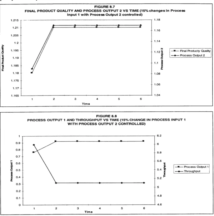
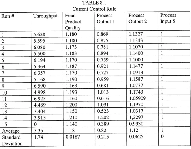
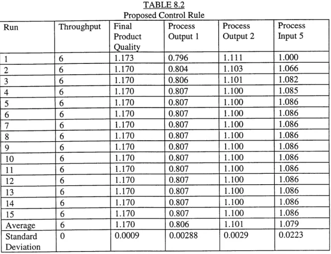
* Kiln Process Output 2 has a higher correlation to final product quality than that of Process Output 1. Furthermore, Process Input 5 significantly affects Process Output 2, is easier to adjust than Process Input 1, and is less disruptive to the process than Process Input 1. Thus, a possible control strategy would be to vary Process Input 5 in response to changes in Process Output 2. The next chapter will further discuss this point.

* The model did not support hypothesis that the differences in the technical features between the European and the North American kilns would affect the sensitivity of the final product quality to variations in the kiln process inputs. For example, the European kiln dimensions and the inlet location of Process

Input 5, which are different for the European kiln from the North American kiln, do not significantly affect the final product quality.

* However, the Process Input 5 inlet location, Process Input 1, Process Input 3, and Equipment Dimension 1 all significantly affect the value of Process Output 3. Since the value of Process Output 3 affects machine downtime, these variables significantly impact the likelihood of machine downtime. * Variations in Dryer Process Inputs 2 and 5 of +/-10% had a statistically

significantly impact on the drying rate.

We will discuss these conclusions in more detail below. We will begin by

discussing the sensitivities of the kiln process inputs to the final product quality. Then, a preliminary investigation of the current control strategy will be completed by using the process input sensitivities. Next, we will discuss the sensitivity of the process outputs to variations in the process inputs. Since final product quality is linked to throughput (low

quality results in low throughput), we can determine the effect of the inputs on throughput. The analysis will be used to learn about the key process inputs and their optimum values.

KILN SENSITIVITY ANALYSIS:

CORRELATION OF PRODUCT QUALITY TO PROCESS INPUTS:

The kiln and dryer models were used to run several half factorial DOEs with four inputs being varied. Each of the inputs was varied among three values (the standard value, high or standard value +10%, and low or standard value -10%) which resulted in 27 runs being made for each half factorial experiment. The data was then regressed

versus different outputs to determine how the inputs affected the outputs. The table below summarizes the regression analysis of the 27 runs.

EFFECT OF PROCESS INPUTS ON PRODUCT QUALITY

Process Input Process Input Process Input Process Input Process Input Process Input Process Input Process Input R2 I coefficient 2 coefficient 3 coefficient 4 coefficient 1 t-ratio 2 t-ratio 3 t-ratio 4 t-ratio

-.000574 .002002 .0296 -.00036 4.57 1.61 4.82 1.90 0.730

These results indicate that Process Inputs 2 and 4 are not significantly related to final product quality with t-ratios of 1.61 and 1.90 respectively (statistical significance was calculated at the 5% level). The coefficients of Process Inputs 1 and 3 have t-ratios greater than 4, which suggest that they are significantly related to final product quality.

CORRELATION BETWEEN FINAL PRODUCT QUALITY AND THE CONTROL VARIABLE:

The model also indicates that product quality is not strongly correlated to the current control variable, Process Output 1. A regression of product quality against Process Output 1 gave an R2 coefficient of only 0.235. This indicates that only 23.5% of the variability in the final product quality is explained by the control variable.

PROCESS OUTPUT 1 CORRELATED TO PRODUCT QUALITY Process Output Process Output R2

1 (the control 1 t-ratio variable)

Coefficient

0.0014815 2.35 0.235

The model also indicates that another process output (Process Output 2) is correlated more strongly to final product quality than Process Output 1. A

regression of product quality against Process Output 2 gives an R2 coefficient of 0.789 and a t-ratio of 8.21. This analysis indicates that controlling to Process Output 2 could be a better control strategy.

PROCESS OUTPUT 2 Process Output 2 Coefficient

0.002061

CORRELATED TO PRODUCT QUALITY Process Output R2

2 t-ratio

8.21 0.789

EFFECT OF PROCESS INPUT 5:

Process Inputs 1, 2, 3, and 5 were varied in a half factorial DOE. The table below gives the coefficient and the t-ratios for the impact of the inputs on Process Output 2. As can be seen from the table, Process Input 5 has a statistically significant effect on Process Output 2. Process Input 5 is easier to vary than the current control variable and has a less disruptive effect on the operations of the process than Process Input 1 (which has a direct effect on throughput). Thus, when devising a control strategy, Process Input 5 could be varied to control Process Output 2. This point will be further discussed in the control strategy chapter.

EFFECT OF PROCESS INPUT 5 ON PROCESS OUTPUT 2

Coefficient Coefficient Coefficient Coefficient t-ratio for t-ratio for t-ratio for t-ratio for for Process for Process for Process for Process Process Input Process Input Process Input Process Input

Input Inut 2 Input 3 Input 5 1 2 3 5

N.A. flows -.2428 1.0319 11.278 -49.778 6.49 2.21 4.82 6.66

and dimensions

SENSITIVITY TO INPUTS WITH DIFFERENT PROCESS EQUIPMENT DIMENSIONS:

There was initially some thought that using the European dimensions of the kiln (e.g. height, radius, etc...) would make the process more robust to variations in process

inputs. The European plant not only uses different equipment dimensions, but also uses different values for the process inputs. First, we will investigate the impact of using the European dimensions while using the North American process inputs values. Then, we will investigate the impact of using the European process input values with the North American dimensions.

As the analysis given below shows, the European dimensions do not reduce the sensitivity of the final product quality to variation in the inputs. The table below gives the results for running the half factorial DOE with the European dimensions. The statistical analysis indicates that each of the process input coefficients impact on product quality is within a standard error of each other in the European dimensions case vs. the North American dimensions case. Therefore, the sensitivities of the process inputs to the final product quality do not change with the European dimensions. Once again, Process Inputs 1 and 3 have a statistically significant impact on the final product quality.

EFFECT OF EUROPEAN AND NORTH AMERICAN DIMENSIONS ON PRODUCT QUALITY

Process Process Process Process Process Process Process Process Input 1 Input 2 Input 3 Input 4 Input 1 t- Input 2 t- Input 3 t- Input 4 t-coefficient coefficient coefficient coefficient ratio ratio ratio ratio N A. -.000574 .002002 .029603 -.00036 -4.57 1.61 4.82 -1.90

dimensions

Euro -.00065 .00203 .02617 -.000269 -4.45 1.57 4.07 -1.31

dimensions

The model ran another scenario that changed only one of the equipment

dimensions to the European value and left the other key dimension at the North American value. The dimension noted as Equipment Dimension 1, is easier to change than

Equipment Dimension 2, so the North American plant could easily change it. The table below summarizes this scenario.

EFFECT OF EQUIPMENT DIMENSIONS ON PRODUCT QUALITY

Process Process Process Process Process Process Process Process Input 1 Input 2 Input 3 Input 4 Input 1 t- Input 2 t- Input 3 t- Input 4 t-coefficient coefficient coefficient coefficient ratio ratio ratio ratio

N.A. -.000574 .002002 .029603 -.00036 -4.57 1.61 4.82 -1.90 Dimensions Euro -.000717 .00159 .030463 -.000195 -4.05 1.02 3.91 -0.78 Dunension I/N A Dimension 2

Once again, each of the differences in the coefficients is less than the standard errors in the coefficients, so there are no statistical differences in the sensitivities between the two cases with respect to the inputs. We concluded that varying the equipment dimensions do not affect the sensitivity of the product quality to variations in the

process inputs.

EFFECT OF EUROPEAN PROCESSING INPUTS:

The effect of the differences between the standard process input values between the European and North American kilns was analyzed using a half factorial DOE. Prior to running the model, we did not know if the different process inputs would interact with the other inputs to change the sensitivities to the inputs. The DOE confirmed that the sensitivity of product quality to Process Inputs 1, 2, and 3 were statistically the same, despite the different values of the process inputs. However, the European values did result in variations to Process Input 4 having less of an impact on final product quality but still having a statistically insignificant impact. The table below compares the results to the current North American case (North American dimensions and North American Process Inputs).

EFFECT OF THE EQUIPMENT DIMENSIONS ON PRODUCT QUALITY Process Process Process Process Process Process Process Process Input 1 Input 2 Input 3 Input 4 Input 1 t- Input 2 t- Input 3 t- Input 4t-ratio

coefficient coefficient coefficient coefficient ratio ratio ratio

N A -.000574 .002002 .029603 -.00036 -4.57 1.61 4.82 -1.90 dimensions Euro -.000558 .00234 .028399 .0000755 -5.53 1.51 4.34 0.30 dimensions with Euro Process Inputs

PROCESS INPUT 5 INLET LOCATION:

One of the European process inputs enters in the middle section of the kiln. The effect of changing this location was investigated. Once again, a half factorial DOE was run in which Process Input 5 inlet location, Equipment Dimension 1, Process Input 1, and Process Input 3 were varied to determine the effect on the kiln operations. A linear regression indicated that the Process Input 5 location had no statistical effect on the final product quality. The coefficients and t-ratios for each of the inputs used in the DOE are given below (R2 for the correlation was 0.891).

EFFECT OF INPUTS ON PRODUCT QUALITY

Coefficient Coefficient Coefficient Coefficient t-ratio for t-ratio for t-ratio for t-ratio for for the for the for Process for Process the Process Equipment Process Input Process Input Process Input Equipment Input 1 Input 3 Input 5 Dimension 1 1 3

5 Location Dimension 1 location

N.A. flows .03074 -.317 -.00083 .0375 1.14 .633 8.31 5.99

and

dimensions

Changing the inputs to the standard European values does affect Process Output 3, which is important because an increase in Process Output 3 increases the likelihood of machine downtime. The table below gives the coefficients and the t-ratios for the effect of the inputs on Process Output 3. (The R2was 0.99 for this regression)

EFFECT OF INPUTS ON PROCESS OUTPUT 3

Coefficient Coefficient Coefficient Coefficient t-ratio for the t-ratio for t-ratio for t-ratio for for the for the for Process for Process Process Input Equipment Process Input Process Input Process Input Equipment Input 1 Input 3 5 Location Dimension 1 1 3

5 location Dimension 1

N.A. 56.56 -580.00 -0.354 19.08 21.34 11.9 36.3 31.33

Process Inputs and

dimensions

As can be seen from the above table, each of these variables is significantly related to this Process Output 3. Thus, these variables can be adjusted to decrease machine downtime.

DRYER SENSITIVITY ANALYSIS:

Now that we have completed the kiln analysis, we will use the models to complete an analysis of the dryer. The dryer model was used to run an L-18 DOE, which

investigated the effect of the inputs on the drying rate. The results indicate that conditions in the drying system where the heat transfer controlled drying region occur have the biggest impact on drying. The process inputs do not have as large of an impact during the conduction/diffusion controlled drying. The statistically significant inputs that impact drying were discovered by completing a sensitivity analysis.

The table given below summarized the results. The drying rate was

significantly affected by variations of +/- 10% from the standard values for Process Inputs 2 and 5. Process Inputs 2 and 5 affect drying in the heat transfer controlled region. The other process inputs which affect the drying conditions in the

conduction/diffusion controlled region of the drying did not have a statistical significant impact on the drying rate. Thus, adjusting the process inputs (except for Process Inputs 2 and 5) will not increase the drying rate.

EFFECT OF THE PROCESS INPUTS ON THE DRYER

Coeffic Coeffic Coeffic Coeffici Coeff Coeffic Coeffic t-ratio t-ratio t-ratio t-ratio t-ratio t-ratio t-ratio

lent for ient for ient for ent for icient lent for ient for for for for for for for for Proces Proces Proces Process for Proces Proces Proces Proces Proces Proces Proces Proces Proces s Input s Input s Input Input 4 Proce s Input s Input s Input s Input s Input s Input s Input s Input s Input

1 2 3 ss 6 7 1 2 3 4 5 6 7

Input

5

Dryer 14.95 -.060 -.001 .0001 .0003 .635 -8.80 1.55 3.05 1.35 0.221 2.08 1.31 0.507

This chapter illustrated the effectiveness of using computer models to complete a sensitivity analysis. This approach enabled us to determine the key process inputs and their interactions with equipment dimensions. Some of the key hypotheses before conducting this analysis were that the European dimensions and process input values decreased the sensitivity of product quality to variations in the inputs, Kiln Process

Output 1 (the control variable) had a high correlation to product quality, and all of the drying process inputs had a significant effect on the drying rate. The use of the model indicated that the sensitivity of product quality to variations in the process inputs was no different with the European Kiln dimensions and process input values than with the North American dimensions and process input values. Furthermore, the results indicate that the correlation between Process Output 1 and product quality is low and that Process Output 2 has a higher correlation with the product quality. Finally, the drying model indicated that optimizing the values of the process inputs that affect the conduction/diffusion controlled drying region will not significantly increase the drying rate. To increase the drying rate, the process inputs that affect the heat transfer controlled region (Process Inputs 2 and 5) must be optimized. In the next chapter, we will use some of these conclusions to develop an alternative control strategy and then the final chapter of the thesis will summarize the key learnings from the entire thesis.