Computational simulation of unsteady flow in transonic compressor rotor

by Philip Ray Owen

GTL Report No. 189 October 1986

This work was sponsored by the Allison Gas Turbine Division of General Motors, and by the Air Force Office of Scientific Research, Multi-Investigator Contract #F49620-85-C-0018, Dr. James D. Wilson Program Manager.

by

PHILIP RAY OWEN

ABSTRACT

The unsteady flow about a section of a modern first stage transonic compressor rotor was simulated using a finite difference approximation to the two-dimensional, Reynolds averaged, unsteady, compressible, viscous Navier-Stokes equations. The computation was performed in both steady

state and time-accurate modes, and the results compared. The time-accurate results were analyzed in some detail. Two frequency regimes were observed. High frequency

unsteadiness due to vortex shedding was found at frequencies varying between 11 KHz and 19 KHz. A low frequency cycle

was also observed at 365 Hz. The low frequency cycle

produced significant variations in blade force and moment. It also modulated the strength and frequency of the vortex shedding.

Arguments were advanced to explain the mechanics of the vortex street formation in terms of a single free shear layer instability. The variations in shedding strength and frequency were related to movement of the separation point. A wholly satisfactory normalization of the frequencies was not found.

The low frequency cycle was analyzed as a quasi-steady sequence of events stemming from movement of a shock wave spanning the blade passage. The possibility was entertained that the cycle was due to purely numerical sources, but no likely mechanism was found.

Abstract . . . . . . .. . . . . .... .. .

... ii

Table of Contents . . . . . . . . . . . . . . . . . . .iii

List of Tables . . . . . . . . . . . . . . . . . . .. . v

List of Figures . . . . . . . . . . . . . . Vi CHAPTER 1 INTRODUCTION . . . . . . . . . . . . . . . . 1

CHAPTER 2 METHOD AND COMPUTATIONAL PROGRAM . . . . . . 3

2.1 Computational Method . . . . . . . . . . . . . . 3

2.1.1 Normalized Equations . . . . . . . . . . . 4

2.1.2 Spatial Discretization and Smoothing . . 6

2.1.3 Time Integration and Stability . . . . . . 8

2.1.4 Boundary Conditions . . . . 9

2.1.5 Handling of Turbulence . . . . . . . . . . 11

2.1.6 Additional Remarks . . . . . . . . . . . . 11

2.2 Method of Investigation . . . . . . . . . . . . 12

CHAPTER 3 AIRFOIL GEOMETRY, HYPOTHETICAL OPERATING CONDITIONS AND COMPUTATIONAL GRID . . . . . 15

3.1 Airfoil Geometry . . . . . . . . . . . . . . .. 15

3.2 Hypothetical Operating Conditions . . . . . . . 16

3.3 Computational Grid . . . . . . . . . . . . . . . 18

CHAPTER 4 STEADY STATE RESULTS . . . . . . . . . . . . 20

4.1 Convergence Behavior . . . . . . . . . . . . . . 20

4.2 Basic Flow Field Characteristics . . . . . . . . 21

4.2.1 Passage Shock

.

.

.

.

.

.

.

.

. .. .. . .

22

4.2.2 Suction Surface Boundary Layer Separation . 23 4.3 Blade Performance . . . . . . . . . . . . . . . 24

5.2 Comparison with Steady State Results . . CHAPTER

6.1

6 HIGH FREQUENCY UNSTEADINESS: VORTEX SHEDDING . . . . . . . . . . .

Strong Shedding

.

.

.

.

.

.

.

.

.

.

.

.

Weak Shedding

.

.

.

.

.

.

.

.

.

.

.

.

.

Frequency Normalization

.

.

.

.

.

.

.

.

Mechanics of Vortex Strength Variation

.

31 36 38

40

Summary

.

.

.

.

42

.

.

.

42

.

.

.

52

.

.

59

.

71

iv

.

Chapter 3

Table 3.1 Summary of NASA Rotor 67 Section 5 Two-Dimensional Meanline Geometry Table 3.2 Hypothetical Operating Conditions

Chapter 4

Table 4.1 Mach Numbers at Cells Along Xsi-Inversion Line 15. Steady State Iteration 2500

Table 4.2 Extent of Shock Smearing Based on Different Shock Start Locations Table 4.3 Overall Blade Performance Averaged 1.6 Trailing Edge Diameters

Downstream of Blade Trailing Edge. Steady State Iteration 2500

Chapter 5

Table 5.1 Time-Accurate Extrema, Time Averages, and Steady State Solution Values

Table 5.2 Time Averages, Total Variations in Time-Accurate Results, and Differences between Steady State and Time Averaged Values Table 5.3 Sensitivity of Adiabatic Efficiency to Small Changes in Total

Pressure and Total Temperature Ratios

Chapter 6

Table 6.1 Sample of Approximate Vortex Core Pressures

Chapter 7

Table 7.1 Distances and Velocities Used in Estimating Extreme Frequencies

Due to Wave Reflection Off the Downstream Computational Boundary Table 7.2 Sample Calculation of Extreme Frequencies Due to Wave Reflection

Off the Downstream Computational Boundary

Chapter 3

Figure 3.1 NASA Rotor 67 Section 5 Blade Shape

Figure 3.2 Pass 45 Grid

Figure 3.3 Pass 45 Grid, Leading Edge Detail

Figure 3.4 Pass 45 Grid, Trailing Edge Detail

Chapter 4

Figure 4.1 Steady State Convergence History Figure 4.2 Steady State Error Locations

Figure 4.3 Mass Flow Variation, Steady State Iteration 2500 Figure 4.4 Mach Number Contours, Steady State Iteration 2500

Figure 4.5 Steady State Shock and Boundary Layer Separation Locations Figure 4.6 Relative Total Pressure vs. Fractional Blade Spacing 1.6 Trailing

Edge Diameters Downstream of Trailing Edge. Steady State Iteration 2500

Chapter 5

Figure 5.1 Segment of Time-Accurate "Convergence" History (Strong Shedding) Figure 5.2 Maximum Change Locations for Convergence History Segment

Presented in Figure 5.1 Figure 5.3 Coefficient of Lift vs. Time

Figure 5.4 Coefficient of Drag vs. Time

Figure 5.5 Coefficient of Moment vs. Time

Figure 5.6 Location of Moment Center Used in Figure 5.5

Figure 5.7 Segment of Time-Accurate "Convergence" History (Weak Shedding) Figure 5.8 Surface Temperature Distributions at Two Different Times

Figure 6.1 Velocity Vectors in the Blade Frame of Reference for Iteration 42500

Figure 6.2 _{Static Pressure Contours from Iteration 42500 Showing} First Pressure Surface Vortex Near Trailing Edge Figure 6.3 Static Pressure Contours from Iteration 42500 Showing

Suction Surface Vortex

Figure 6.4 Static Pressure Contours from Iteration 42500 Showing Second Pressure Surface Vortex

Figure 6.5 Velocity Vectors from Iteration 42500 in Frame of Reference of First Pressure Surface Vortex

Figure 6.6 Velocity Vectors from Iteration 42500 in Frame of Reference of Suction Surface Vortex

Figure 6.7 Velocity Vectors from Iteration 42500 in Frame of Reference of Second Pressure Surface Vortex

Figure 6.8 Locations of All Vortex Centers Found in Solutions Stored from Iterations 42000 through 43500

Figure 6.9 Vortex Core Locations at Iteration 42250 Figure 6.10 Vortex Core Locations at Iteration 42500 Figure 6.11 Vortex Core Locations at Iteration 42750 Figure 6.12 Typical Suction Surface Separation Location

Figure 6.13 Locations of All Vortex Centers Found in Solutions Stored from Iterations 61250 through 62000

Figure 6.14 Vortex Core Locations at Iteration 61250

Figure 6.15 Schematic of Hypothesized Vortex Shedding Mechanics

Figure 6.16 Normalized Frequency Parameter and Actual Shedding Frequencies Figure 6.17 Normalized Frequency Parameter vs. L/6*

Figure 6.18 Schematic of Vortex Strength Variation with Separation Point Location

Figure 6.19 Calculation of Average Local Boundary Layer Vorticity Figure 6.20 Separation Point Location with Regions of Strong and Weak

Vortex Shedding as Shown by Trailing Edge Static Pressure Fluctuations

Figure 7.1 Distances Used in Estimating Extreme Frequencies of Oscillation Due to Wave Reflection Off the Downstream Computational Boundary

Figure 7.2 Xsi-Inversion Lines Examined in Estimating Extreme Frequencies of Oscillation Due to Wave Reflection Off the Downstream Computational Boundary

Figure 7.3 Times Selected in Estimating Extreme Frequencies of Oscillation

Due to Wave Reflection Off the Downstream Computational Boundary (Relative to Airfoil Moment Variation)

Figure 7.4 Relevant Frequencies in Time-Accurate Simulation of Flow in NASA Rotor 67 at 60 Percent Span

Figure 7.5 Axial Velocity Along Xsi-Inversion 5 at Iteration 42500 Figure 7.6 Relative Total Pressure Observed by a Stationary Observer

Downstream of NASA Rotor 67 at Approximately 60 Percent Span. Comparison of Experimental and Computational Results

Figure 7.7 Maximum Mach Numbers Along Xsi-Inversion Lines 5, 15, and 25 Figure 7.8 Extreme Locations of Sonic Line and Separation Point

Figure 7.9 Separation Point and Maximum Mach Number for Xsi-Inversion 5 Figure 7.10 Calculation of Boundary Layer Vorticity Flux in Unsteady Flow Figure 7.11 Vorticity Flux From Suction and Pressure Surfaces

Figure 7.12 Separation Point Velocity and Suction Surface Vorticity Flux

Figure 7.13 Airfoil Circulation and Lift

The flow through the compressor stage of a gas turbine engine is inherently unsteady in the laboratory frame of reference. For the purpose of designing and analyzing these machines, it is traditional (and a tremendous simplification) to assume that the unsteadiness is purely due to the rotation of the compressor rotor, i.e. that the flow relative to the compressor blades themselves is steady. It has become apparent, however, that even in the blade-relative frame there is considerable unsteadiness in the flow. This has been documented especially by Ng in [1.1] and [1.2], and by Gertz in [1.3] by use of high frequency response instrumentation. As the nature of this unsteadiness becomes better understood, it is expected that the time-averaged performance and reliability of gas turbine compressors may potentially be improved by accounting in the design process for the unsteadiness.

The measurements taken to date, however, have given only a limited view of the actual blade-relative flow field. Indeed, it is impossible to fully construct many flow details from information sampled at a single location (or small number of locations) behind a rotating compressor rotor. Ng hypothesized a high frequency vibration of the rotor shock wave as a cause of much of the unsteadiness he observed. Gertz hypothesized the presence of a vortex street in the blade wakes and constructed a model of such a flow which agrees qualitatively (and in several quantitative respects) with his data. Additional information about the validity of these hypotheses and about other flow details is needed in order for a better understanding of blade-relative unsteadiness to be gained and effectively used.

direct measurement of additional unsteady flow phenomena in the turbomachinery environment. For the present, however, resort has been made to computational simulation of the flow fields in question. Time-accurate computational results have been published by Scott in [1.4] and by Scott and Hankey in [1.5]. These efforts have focused on the effects of upstream unsteadiness such as are created by the wakes of stationary guide vanes entering the rotor flow field. The results obtained by Ng and Gertz, however, show blade-relative unsteadiness behind fan rotors the flow upstream of which is steady. The interest in blade-relative unsteadiness for cases in which the upstream flow is steady has led to the present study.

The objective of this work is to numerically simulate the two-dimensional unsteady blade-relative flow field of a modem transonic compressor fan rotor and examine in some detail the nature of the unsteadiness observed. Chapter 2 surveys the computational algorithm used and the general method of investigation. Chapter 3 discusses details relating to the specific case studied. Chapter 4 presents the steady state results for this case. Chapter 5 is an overview of the unsteady results obtained which introduces the two frequency regimes observed. Chapters 6 and 7 discuss in more detail the high and low frequency cycles respectively. The final chapter summarizes the conclusions drawn from this work together with some suggestions for further study.

CHAPTER 2 METHOD AND COMPUTATIONAL PROGRAM

2.1 Computational Method

Chapters 4 and following present results and analysis of results from a numerical simulation of a compressor flowfield. The program used for this simulation is called ANSI2D. It is a discrete iterative approximation to the Reynolds averaged, unsteady, compressible, viscous Navier-Stokes equations in two-dimensions. It is capable of seeking either steady-state or time-accurate solutions. ANSI2D is an explicit algorithm derived from an earlier implicit scheme discussed in [2.1].

Like its implicit predecessor, ANSI2D regards state vectors to be stored at cell centers rather than at grid nodes. This allows for a variety of grid topologies (including sheared grids with imbedded C-grids and/or O-grids) to be conveniently handled by the algorithm. The program calculates discrete differences along lines connecting cell centers, called inversion lines, two of which pass through each grid cell. Cross-passage inversion lines are called eta-inversion lines; the others (which run in a generally streamwise direction) are called xsi-inversion lines. Values at cell faces are obtained by interpolation between the appropriate cell-centered state vectors.

ANSI2D is also like the implicit scheme discussed in [2.1] in its treatment of boundary conditions. A dummy cell is created on the opposite side of the boundary from each interior boundary cell. The flow properties at the boundary are obtained by interpolation between the interior boundary cell and its dummy cell just like values at any interior cell face are obtained. A subroutine for the appropriate boundary type (inflow, outflow, or solid wall) assigns a value to the state vector for each dummy cell such that the properties interpolated

for the boundary satisfy the appropriate boundary conditions.

ANSI2D is fully documented in [2.21 The following sections provide a brief summary of its main features. Where program options are available, emphasis is placed on those options chosen for the present work.

2.1.1 Normalized Equations

The unsteady Navier-Stokes equations are normalize as follows:

x'=x/L y'=y/L t'=tcTO/L

u'=u/cTO v' =v/cTO _IP/1TO

p'I=p/pTO PV=/. TO T =T/TTO

where L is the blade axial chord, cT O is the upstream stagnation speed of sound, and y is the ratio of specific heats. The subscripting () T denotes an upstream stagnation quantity. All quantities are in the blade relative frame.

The bulk viscosity in the Navier-Stokes equations is defined using Stokes' hypothesis that X=-21/3

The resulting equations, expressed in conservation form with primes dropped, are as follows:

U + F + G

where, Pu 2 Pu' +p+o F= PUV+T xy puH+ua x+VT xy +qx ax- 2 yu+L- - 2 Ru x 3Re 3x Dy Re x Pv PUV T YX 2 pv +p+a puH+uT +VcY+ yx yY a _ 211 (_u+v 2p v y -Re x y Re y T =T

xy yx =

_~e

E = + (u2+V2)

Y-1 P 2 H = E + _p = _Y-1 Y-+ _P 2I(U2 +V2

Re is the upstream "stagnation Reynolds number" defined as Re = pTO CTOL/1JTO

Pr is the Prandtl number whose value for liminar and turbulent flow is specified by the user. In this work the laminar Pr is taken as 0.72; the turbulent Pr as 0.90.

The equation of state is the perfect gas law which, with the above normalization, reduces to p = pT/y

Viscosity is calculated using Sutherland's law which normalizes to

T /

= + S

T + S

where S is the normalized Sutherland reference temperature which is specified by P Pu Pv pE and, x

the user. In this work it is taken to be 1990 R/Tro.

2.1.2 Spatial Discretization and Smoothing

The equations of motion given above are integrated over a closed region R producing the following.

- U dA +ff (Fn + Gny) ds = 0

t R _R:

where n, and n, are unit vector components facing outward from the boundary of R. Each grid cell is then regarded as an integration region R.

Discretization is performed by regarding each cell as small enough so that the flux quantities, F and G, may be taken as uniform over the cell face, and the state vector properties at the cell centers taken as uniform throughout the cell. This is known as the finite volume approach. Details are given in [2.21

The discretization is such that all flux properties at a given cell's faces are determined only from state vector properties at that cell and its immediate neighbors. This results in the basic algorithm being unable to detect or damp non-physical "sawtooth" oscillations of flow properties in the solution. Consequently, numerical smoothing must be added to the algorithm to damp these oscillations. Three types of smoothing are available: fourth-order,

second-order, and implicit.

Fourth-order smoothing makes use of information from cells two removed from a given cell and hence is very effective in eliminating sawtooth oscillations. It has been observed by various researchers, however, that in the neighborhood of strong gradients, such as shocks, fourth-order smoothing is undesirable.

Second-order smoothing makes use of information only from a cell's nearest neighbors and is preferable to fourth-order smoothing in the neighborhood of strong gradients.

The smoothing formulation in ANSI2D allows use of both fourth- and second-order smoothing in varying proportions for different spacial locations. In the vicinity of strong pressure gradients such as would be produced by a shock the program automatically decreases the amount of fourth-order smoothing while increasing the amount of second-order smoothing. Again, details are given in [2.2].

For time accurate running, it has been found suitable to eliminate use of second-order smoothing entirely for the present work. Since the flow field does include a shock, this means there is very little smoothing at all applied near the shock. The shock is thus made as clearly defined as possible. No undesirable oscillations have been observed in the solution. Fourth-order smoothing was, by trial and error, set to a value believed to be near the

minimum required for stability of the algorithm.

Implicit smoothing is applied to the discrete time integration step to

inhibit the formation sawtooth oscillations. It is suitable only for steady-state running. It requires the solution of a tri-diagonal system of equations twice for each cell (once for the xsi-inversion line passing through the cell and again for the eta-inversion line). It requires approximately 15

percent more CPU time per iteration, but allows the discrete time step to be increased significantly - by a factor of 5 in the present work. Thus, implicit smoothing was used to advantage (along with minimal fourth-order smoothing) in obtaining steady-state results.

2.1.3 Time Integration and Stability

The spatial discretization outlined above produces a system of ordinary differential equations in time. These may be symbolically written as

d

d (AkUk) + Rk (U) = 0

where the subscript OK indicates cell k, AK is its area, U is the vector defined in section 2.2.1, and R K is a non-linear function of U at cell k and its neighbors corresponding to the spatial flux balance, second-, and fourth-order smoothing.

Two methods are offered in ANSI2D for the discrete integration of these equations. The first, dubbed "second-order Runga-Kutta", is a two-step predictor/corrector. This is the method used for the present work. The second method, a modified "fourth-order Runga-Kutta" is discussed in [2.21

With either method, as for all explicit schemes, there is a limitation on the size of the time step to preserve stability of the algorithm. The physical interpretation of this limitation for the present scheme is as follows. The spatial discretization approximates the flux balance for a given cell only from information at that cell and its nearest neighbors. This flux balance determines the flow properties at the cell at the next time leveL Consequently, information can only be transmitted over the spatial distance of a few cells from one time step to the next. In real flows information is transmitted at a maximum rate of c-+u, the local speed of sound plus the local flow velocity. Thus, the discrete time step must be less than A L/(c+u), where AL is the maximum linear dimension of the cell.

As indicated by the title of [2.21 ANSI2D was originally developed to solve the steady-state Navier-Stokes equations. This was to be done by

integrating only approximately in time. Since the stability requirement is tied to the local cell size, a variable time step was to be used: large time steps for the large cells in the inviscid part of the flow, small time steps for the small cells in the boundary layer. This is, in fact, the steady-state mode of operation, and it was employed to obtain the steady-state results to be presented later.

For time-accurate running, however, it is necessary to use a constant time step throughout the flow field. This limits the size of the time step to that associated with the smallest cell in the grid, a very small value. Consequently, a great number of iterations and a large amount of CPU time have been necessary to obtain the unsteady results to be presented. Approximately

150,000 iterations requiring roughly 1,364 hours (57 days) of CPU time on a Perkin-Elmer 3240 minicomputer have been necessary to simulate about 8 milliseconds of real flow time. The Perkin-Elmer 3240 is roughly equivalent in

speed to a VAX 11/780.

2.1.4 Boundary Conditions

Four types of boundary conditions exist in the present work: those associated with the inflow grid boundary, the outflow grid boundary, the blade surface, and the interblade passage boundaries. These will be discussed separately in the following paragraphs.

The program normalizes most flow properties to values associated with blade-relative stagnation quantities at the inflow boundary (see section 2.2.1) which are taken as uniform along the boundary and constant in time. The user specifies the "stagnation Reynolds number" at the inflow boundary. The flow angle (also uniform and constant in time) is specified as well. The "unique

incidence principle" for supersonic cascades (see [2.3]) precludes the specification of flow angle for supersonic inflow conditions. Thus, in its present form, ANSI2D can be used to simulate subsonic inflow conditions only. This proved to be a significant limitation in the present work, and will be discussed further in Chapter 3. Regions of supersonic flow in the interior of the computational domain pose no problems, and do in fact exist in the results to be presented.

The outflow boundary condition is uniform and time constant static pressure. This value of static pressure is specified by the user. This boundary condition is not physically realistic for individual stages of multistage turbomachines, although a better alternative is difficult to construct. In the present work, the outflow boundary has been placed far enough downstream of the blade trailing edge (about 1 chord) so that it is hoped the uniform static pressure condition does not obscure physical characteristics of the real flow in a turbomachinery environment. As will be discussed later, it is believed that this goal has been achieved.

The boundary condition at the blade surface is the usual no-slip, no-throughflow condition. ANSI2D allows the user to specify the blade surface to be either adiabatic, or to have a specified constant temperature. In the present work the adiabatic condition has been chosen.

ANSI2D models the flow in a cascade of blades though only calculating the flow in a single blade passage. It does so by imposing periodic boundary conditions on the interblade passage boundaries. This affects the applicability of calculated results to real turbomachinery flows because it eliminates all unsteady flows in which there is a blade to blade phase difference in unsteady events. That is, ANSI2D can only predict flows in which time varying events occur exactly in phase for all blades in the cascade. This problem is

unimportant for flows in which blade to blade interactions are small.

2.1.5 Handling of Turbulence

ANSI2D assumes turbulence to be limited to the boundary layers and simulates it by an increase in the coefficient of viscosity. In effect, then, ANSI2D approximates the unsteady Navier-Stokes equations after they have been Reynolds averaged only over the short time scales associated with turbulence.

The turbulent viscosity is approximated by a "zero equation" (algebraic) model discussed briefly in [2.4]. Specific parameter values are given in [2.2].

The user must specify fixed locations on the blade surface where transition to turbulence is taken to occur. The estimated turbulent viscosity is added to the molecular viscosity at and after these specified locations (one for the pressure surface, one for the suction surface). The present code does not allow for user-specified re-laminarization. To avoid non-physical gross separation from separating laminar boundary layers near the leading edge, the transition locations have both been placed very near the leading edge in the present work (less than 1 leading edge diameter downstream of the axial leading edge).

2.1.6 Additional Remarks

Shocks are handled by smearing the change in flow properties over several grid cells. No automated grid adaptation or shock capturing features are present in the scheme. The Rankine-Hugoniot relations are satisfied sufficiently well for most applications. As mentioned in section 2.2.2, a minimum of smoothing was used in the vicinity of the shock allowing it to be as

sharply defined as possible. In the present work, it appears that flow changes corresponding to the shock are smeared over about 5 grid points. This is discussed somewhat further in section 4.2.1.

The presence of numerical smoothing tends to diffuse calculated propagating structures more quickly than would occur in real flows. The smoothing formulation allows roughly stationary regions of strong gradients, such as shocks, to remain undiminished. Other structures involving significant gradients of flow properties, such as shed vortices, are also allowed to form, and are a prominent part of the results to be presented. However, these structures become unrecognizably diffuse within about a 1/4 chord downstream of the blade trailing edge. In real turbomachinery flows, experimental results suggest that such vortices may persist for several chord lengths.

2.2 Method of Investigation

After selecting a compressor airfoil geometry and generating a suitable computational grid (see Chapter 3), ANSI2D was run in steady-state mode until reasonable convergence was obtained (see Chapter 4). The program was then run in time-accurate mode using the steady-state solution as a starting point.

ANSI2D produces two outputs: (1) a new flow field file (solution file) available after each time step (i.e. after each iteration), and (2) a convergence history file (updated after each iteration). The convergence history file contains five pieces of information for each iteration: (1) the iteration number, (2) the root-mean-square (RMS) change in flow properties over the entire spatial domain from the preceding solution to the current one, (3) the largest change in flow properties at any computational cell from the preceding solution to the current one, (4) the location of this largest change,

and (5) the quantity (p , pu, pv, or pE) in which this largest change occurred. In steady-state mode it is expected that the changes in flow properties from one iteration to the next will eventually approach zero. Hence the convergence history file gives the level of error present in the computational simulation after each iteration. In time-accurate mode the program is capable of simulating unsteady flow fields. Hence in this case the convergence history file does not necessarily indicate the error level, but only the level of unsteadiness in the flow simulation. As will be shown later, the time-accurate convergence history is useful in determining the frequency of periodic flow field changes.

It was unnecessary to examine the solution file after every iteration in order to adequately analyze the time-accurate results. Further, saving solution files for every iteration would require prohibitively large storage space. Therefore, solution files were saved after every 250 iterations. This provided adequate time resolution for the analysis.

Time-accurate running of ANSI2D was generally done in segments of 2500 iterations. Each segment required approximately 23 hours of CPU time to complete on a Perkin-Elmer 3240 minicomputer, and saved 10 solution files on disk.

Certain information was extracted from each solution file and appended to other files which remained on disk. Analysis of these files yielded complete time histories of certain flow field properties. The information extracted was

the following:

1. Pressures over the entire surface of the airfoil. From these the force and moment on the blade (neglecting skin friction) could be calculated at each time level.

2. All basic flow properties along specified inflow and outflow boundaries. From this information many things could be calculated including mass averaged and "stream-thrust averaged" quantities at each time level, time averaged quantities along each boundary, and simulated readings from a stationary probe. These calculated quantities could be presented in either the relative frame or in a hypothetical absolute frame of reference.

3. Boundary layer separation point locations, and vorticity flux at selected locations along the blade.

4. Maximum Mach numbers along selected streamwise lines. Since the flow field included a cross-passage shock, this information gave an indication of the time varying shock strength and location.

5. Skin friction, temperature, and temperature gradient normal to the wall over the entire surface of the airfoil.

After this information was extracted from the solution files were copied onto magnetic tape convergence history file was also copied onto tape. these files were then deleted from disk storage iterations initiated.

solution files on disk, the for permanent storage. The To conserve disk space and another segment of 2500

CHAPTER 3

AIRFOIL GEOMETRY, HYPOTHETICAL OPERATING CONDITIONS, AND COMPUTATIONAL GRID

3.1 Airfoil Geometry

The airfoil modeled in the present study is a section of the NASA Low-Aspect-Ratio first stage fan rotor reported on in [3.1]. This rotor will be referred to as NASA Rotor 67. The rotor has a hub-to-tip radius ratio of 0.375

at its inlet and 0.478 at its exit. Its aspect ratio is 1.56. Its design speed is 16042.8 RPM. It has been tested in NASA Lewis's steady-state test rig at 103 percent corrected speed with a mass flow of 34.03 kg/sec (75.0 lbm/sec) and developed a total pressure ratio of 1.686 with an adiabatic efficiency of 0.906. These conditions correspond to a tip relative Mach number of 1.31.

This rotor was chosen because extensive unsteady experimental data have been taken on it by Gertz [3.2]. Most of this data is at a location 60 percent of the blade span from the hub. This location corresponds approximately to blade section 5 in [3.1]. A location such as this, near mid-span, is also the flow region most likely to approximate two-dimensional flow.

Blade section 5 is defined in [3.1] on a shallow cone of inclination -2.073 degrees from horizontal. This approximates a streamline location obtained from a streamline curvature calculation. A cone cannot be exactly unwrapped into two dimensions. This section has been unwrapped in such a way as to preserve the most important geometric parameters. The section is defined by a double circular arc meanline and a thickness distribution. The two-dimensional meanline was constructed by preserving the given inlet angle, outlet angle (hence total geometric turning), axial chord, the ratio of the two radii

describing the meanline, and the fraction of the axial chord at which these radii meet. Since the cone is shallow, all other geometric parameters, including setting angle and total chord, are closely approximated. Table 3.1 summarizes the resulting two-dimensional meanline geometry.

The only thickness information given in [3.1] is the leading edge thickness (diameter of leading edge arc), trailing edge thickness, the difference between the meanline angle and the suction surface angle at the leading edge, the maximum thickness, and the axial location of the maximum thickness. A polynomial fit consistent with these data was used to complete the thickness distribution. The maximum thickness to total chord ratio is 4.55 percent. Figure 3.1 shows the final blade shape.

3.2 Hypothetical Operating Conditions

As implied above, an original goal of this research was to compare computational results with experimental data for similar operating conditions. The inlet relative Mach number at 60 percent span for the conditions reported in [3.2] is approximately 1.17. However, as mentioned in section 2.2.4, ANSI2D is not capable of handling a supersonic inflow condition. To remedy this would have involved formulating a new inflow boundary treatment, writing a new subroutine for ANSI2D, and testing the resulting code on cases in which the physical flows are known. Instead, a direct comparison against the data of [3.2] was forfeited in favor of running ANSI2D unmodified with a high subsonic inflow Mach number.

At a variety of off-design conditions, NASA rotor 67 does operate with subsonic relative Mach numbers at 60 percent span. One such case (at 100 percent speed) was modeled early in the research program. However, the

resulting calculated flow field was complicated by large scale separation from the leading edge. This is probably due to one or both of the following considerations: (1) this flow had a high leading edge incidence angle of about 6 degrees, and (2) the turbulence transition locations for this case were set away from the leading edge at roughly mid-chord. It was decided that a simpler flow field was desirable as a baseline case. The leading edge separation was eliminated by specifying an inlet flow angle giving zero incidence at the leading edge, and by moving the turbulence transition locations very near the leading edge (see section 2.2.5).

ANSI2D normalizes calculated flow quantities to inflow relative stagnation quantities. A particular real flow can be contemplated by assigning values to these reference quantities. Further, the rotor can be imagined to be rotating at a certain speed. Hypothetical absolute conditions can then be found which correspond to the imagined relative stagnation conditions.

This has been done for the calculated results to be presented. The complete hypothetical operating conditions are given in Table 3.2. The inlet quantities are the most significant values in the table, especially the inlet relative total quantities (PT, IT, MUT). It is to these values that quantities calculated by ANSI2D are taken to be normalized to in the chapters that follow. For example, all frequencies to be reported are based on these hypothetical conditions. (When values such as velocities or pressures are reported later with no units given, however, they are normalized values as defined in section 2.1.1.) Notice that the rotor is taken to be running at an atmospheric pressure slightly above sea-level standard (15.056 psi) on a cool day (510.00 - 459.67 = 50.33 degrees F) at 100 percent corrected speed. Prewhirl vanes are imagined to be in front of the rotor which turn the incoming flow through 24.399 degrees so that the relative flow angle is 56.810 degrees. Since the leading edge meanline blade angle is 56.810 degrees, this gives a zero incidence condition. The

relative Mach number is about 0.92. The relative Reynold's number is

6 (

1.17x10 based on the axial chord. Based on the true chord it is 1.83x10

The exit conditions shown in Table 3.2 correspond only approximately to those produced by ANSI2D. They were obtained by satisfying continuity of mass flow from inlet to exit given a value for the loss of relative total pressure (0.97 in this case which is near the value predicted by ANSI2D). If these conditions were actually observed, the rotor section would be operating with a total pressure ratio of 1.29 at an adiabatic efficiency of 88.9 percent.

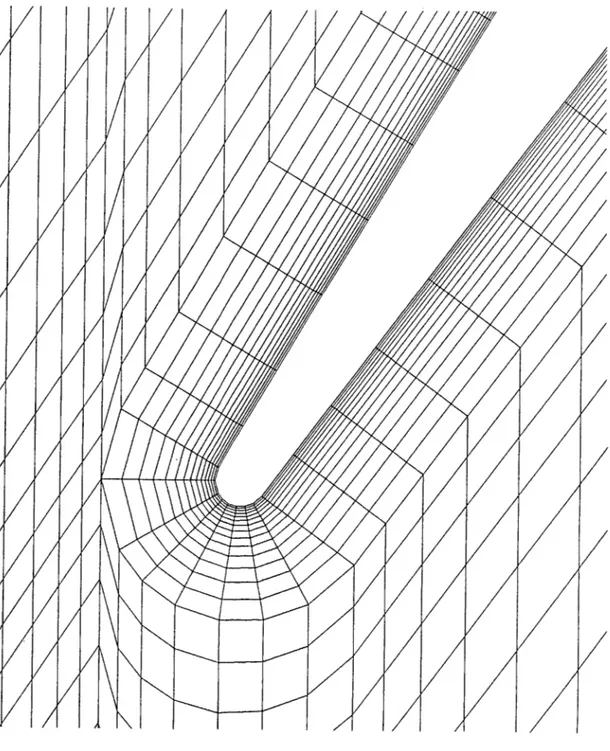
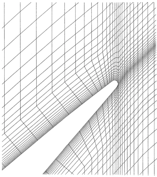
3.3 Computational Grid

The grid used in this work is a sheared grid with a C-grid imbedded to better resolve the blade boundary layers and wake. It is shown in Figure 3.2. Enlargements of the leading edge and trailing edge regions are shown in Figures 3.3 and 3.4. These figures show the grid cells; the inversion lines pass through the centers of these cells.

The outermost line in the C-grid was defined by a crude estimation of the boundary layer growth based on expected operating conditions. Fifteen grid lines (giving 14 xsi-inversion lines) were placed in the C-grid. They are exponentially spaced giving greatest resolution near the blade surface.

The location of the grid boundary layer edge is only significant in the turbulence modeling. The molecular viscosity is augmented by the estimated turbulent viscosity only within the grid boundary layer. The equations of motion solved by ANSI2D are always the Reynolds averaged Navier-Stokes equations; the boundary layer approximation is not employed. In the present work the boundary layer thickness for both surfaces near the trailing edge was

underestimated. In this region the velocity parallel to the blade surface reaches its "free stream" value approximately twice as far from the blade surface as the last inversion line in the C-grid.

The sheared grid fills in the upstream space and the core flow region between the blades and wake. It has 28 streamwise lines (giving 29 xsi-inversion lines) which are also exponentially spaced so as to give the greatest resolution near the boundary layer edges. Care was taken to avoid a large change in cell size at the junction between the sheared grid and the

C-grid.

The cross-passage grid lines (defining the eta-inversion lines) were spaced

so as to adequately resolve the leading and trailing edges and yet keep the

overall number of grid cells reasonable. Exponential spacing was used where needed to provide smooth transitions in cell size.

The final grid (dubbed the "Pass 45 Grid") has 7108 interior cells and 226 boundary cells for a total of 7334 cells. There are a total of 57 xsi-inversion lines running in the streamwise direction within the bladed region: 14 in each boundary layer, 29 in the core. There are a total of 136 eta-inversion lines (running cross-passage), 70 of which are in the bladed region.

CHAPTER 4 STEADY STATE RESULTS

4.1 Convergence Behavior

ANSI2D must always start its iterations toward a solution from a file which approximates the flow field. Usually this is a solution file generated previously by ANSI2D. However, to start the program on a new grid it is necessary to generate the "initial solution" file artificially. The steady state iterations were started from such a file in which the flow conditions were only crudely approximated. The flow direction was made constant throughout the region outside the grid boundary layers. The inlet Mach number and exit Mach number were specified, and interior Mach numbers linearly interpolated from these. An approximate boundary layer velocity profile was generated within the grid boundary layers.

ANSI2D was started in steady state mode (variable time step) from this solution. The local CFL number was specified as 4.0, the second-order smoothing coefficient set at 0.0, the fourth-order smoothing coefficient set at 0.075, and the implicit smoothing coefficient set at 4.0. The use of implicit smoothing allows the large (greater than 1) local CFL number.

Figure 4.1 shows the convergence history for the first 2500 iterations. It is observed that the error reaches a minimum after about 1700 iterations and then fails to converge further. In fact, the error tends to increase after 1700 iterations. Experience has shown that the level of convergence never improves significantly beyond this no matter how many iterations are performed.

Figure 4.2 shows the locations of the maximum errors for the first 2500 iterations. The figure is understood as follows. After each iteration ANSI2D

identifies the cell at which the maximum change in flow properties occurred from the previous iteration. A square symbol is plotted in Figure 4.2 at this cell. The same cell may be the location of the maximum change for other iterations as well. This is indicated in Figure 4.2 by the size of the square symbol. A large square indicates that the cell in question was often the site of maximum error; a small square indicates that the maximum error occurred at the marked cell only a few times. Figure 4.2 is thus a sort of two-dimensional histogram of the steady state error.

There are small symbols scattered throughout the flow field in Figure 4.2, most of them in or near the boundary layer region, which indicate adjustments made to the starting "solution." It is evident, however, that the trailing edge is the site of the vast majority of the error. This is typical of flow fields in which vortex shedding is present. The physical presence of vortex shedding means that the flow is inherently unsteady: the Navier-Stokes equations have no steady state solution for such a flow (or if a mathematical steady state solution exists, it is unstable). Consequently, a steady state approximation to the Navier-Stokes equations will never fully converge, the error locations being predominantly near the shedding location (the blade trailing edge in this case).

The failure of the algorithm to converge in steady state is demonstrated by the variation in mass flow rate through the passage, shown in Figure 4.3. The total variation upstream of the trailing edge is slightly less than two percent. The variation near and downstream of the trailing edge is over three percent. This variation does not decrease to satisfactory levels with more iterations.

4.2 Basic Flow Field Characteristics

nevertheless displays the same basic flow phenomena as are found in the time-accurate solutions. The most important of these are the passage shock and its effect on the suction surface boundary layer.

4.2.1 Passage Shock

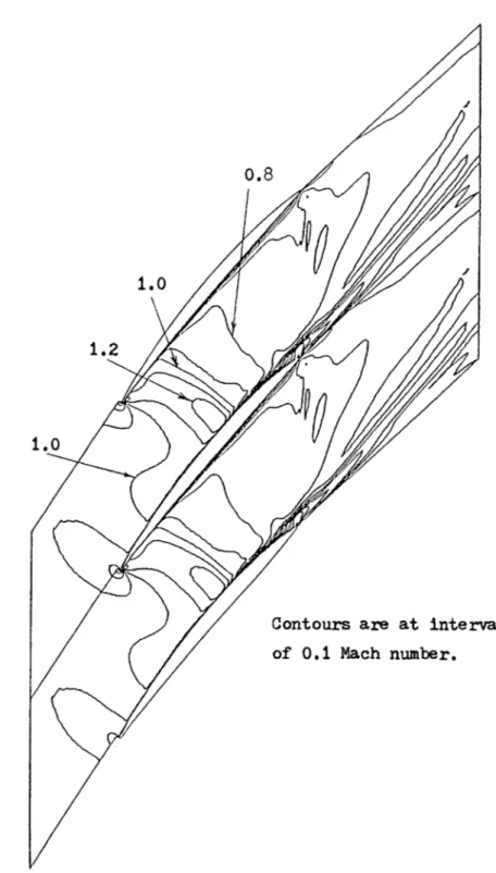
Figure 4.4 is a contour plot of Mach number for iteration 2500. As indicated by the sonic line, a shock extends across the entire passage approximately from the 1/4 chord point on the pressure surface to the 3/4 chord point on the suction surface. The shock may be considered normal to the flow. Its strength varies across the passage being strongest near the suction surface. The maximum pre-shock Mach number there is 1.286 and decreases to 1.207 at mid-passage, and 1.169 near the pressure surface. The complicated nature of the contour lines downstream of the trailing edge is evidence of the lack of full steady state convergence.

The shock arises from the passage area becoming critical (probably due to growth of the boundary layers). Figure 4.4 shows that the flow is sonic or nearly so across the passage at the inlet throat and shocks about 1/4 chord further downstream. It is emphasized that the far upstream flow conditions are subsonic, and thus that the shock is not a bow shock or a swallowed shock as are found in supersonic compressors.

Determining the actual strength of the shock is complicated by its being smeared over several grid cells. The problem will be illustrated by considering the shock at mid-passage. Table 4.1 lists the local Mach numbers at each cell along a segment of xsi-inversion line 15 (the mid-passage streamwise line through cell centers). Suppose the shock is considered to begin at cell 53. Using the normal shock relations, the post-shock flow conditions can be found

based on the Mach number, pressure, and temperature at cell 53. Flow conditions at the cells downstream of cell 53 can then be compared against the expected values until the best match is found. At each cell there will be an error in the Mach number, pressure, and temperature compared to the expected values. The root-mean-square (RMS) of these errors gives an indication of the overall error. The downstream cell at which the RMS error is minimized is considered to be the termination of the shock. This process can be repeated considering cells other than 53 to be the beginning of the shock. The results are shown in Table 4.2.

The normal shock relations are best satisfied by considering the shock to be smeared over five cells from cell 55 to cell 60. This corresponds to a physical normal shock with pre-shock Mach number of 1.164. The shock is smeared over a linear distance of approximately 0.085 blade chords. The difference in flow angle between cells 55 and 60 is 1.4 degrees. This turning would be produced by an oblique shock at an angle of 84.8 degrees. The normal shock approximation is thus considered to be justified.

4.2.2 Suction Surface Boundary Layer Separation

Whereas the pressure surface boundary layer remains attached until the blade trailing edge, the suction surface boundary layer separates. Figure 4.5 shows the location of this separation (as indicated by zero surface shear stress) together with the approximate smeared shock location. The separation occurs slightly downstream of the shock and is thus not properly termed "shock-induced." This is more evident in the time-accurate results in which the movement of the separation point does not follow the movement of the shock. There is little doubt, however, that the shock hastens the boundary layer separation.

4.3 Blade Performance

Average values on which to base statements of overall blade performance have been obtained using two methods. The first is the familiar process of mass averaging. The second will be referred to as "stream-thrust averaging." The fluxes of mass, momentum, and energy are obtained by integrating the non-uniform flow conditions at a given location. A uniform flow is then solved for which has these same fluxes, with pressure differences accounted for in the momentum equations. The average flow thus calculated is what would result if the actual non-uniform flow were to mix out in a constant area duct.

Table 4.3 presents the overall blade performance obtained by both averaging methods applied at an axial location 1.6 trailing edge diameters downstream of the trailing edge. Absolute quantities are based on the hypothetical operating conditions discussed in section 3.2. Depending on the averaging method employed, the blade section produces a total pressure ratio of 1.292 or 1.280. The meanline blade exit angle is 43.24 degrees. Therefore the relative exit flow angle of either 48.59 or 51.84 degrees reflects a deviation angle of 5.4 or 8.6 degrees respectively. The stream thrust averaged efficiency is 90.1 percent, more than two points lower than the mass averaged value of 92.8 percent. This is typical of stream thrust averaging, and tends to more accurately indicate the true performance in an engine environment. The non-averaged variation in relative total pressure at this station is shown in Figure 4.6.

Blade forces and moments (from integration of surface pressures) are also known for the steady state solution. The presentation of these will be delayed, however, because they are more insightful when viewed in comparison with the time-accurate results.

CHAPTER 5 OVERVIEW OF UNSTEADY RESULTS

Time accurate running was initiated from a steady state solution. ANSI2D was allowed to run for a number of iterations corresponding to about two computational domain through-flow times before the time-accurate solutions began to be saved for analysis. The unsteady results to be presented are thus thought to be due to more than merely computational transients from the unconverged steady state starting solution. The starting solution did, however, provide a large perturbation to excite instabilities or natural frequencies in the time-accurate flow.

5.1 General Nature of the Unsteadiness

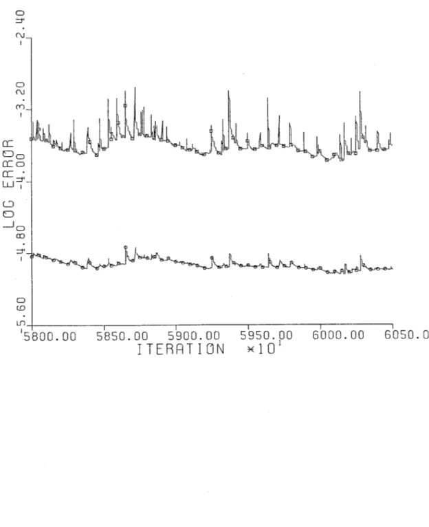
A segment of the time-accurate "convergence" history is shown in Figure

5.1. Unlike the steady state convergence plot, this is not a plot of error level. Figure 5.1 shows the maximum and RMS changes from one iteration to the next. In time-accurate running this is simply an indication of the unsteadiness of the flow. Note that periodicity is evident. The primary usefulness of these plots is in determining from this periodicity the frequencies of the vortex shedding (discussed in Chapter 6). The locations of maximum changes are shown in Figure 5.2. As expected, the greatest unsteadiness is near the blade trailing edge.

The most significant aspect of the time-accurate results to be presented is the presence of two distinct frequency regimes. The high frequency variations are due to vortex shedding. This phenomenon (discussed in detail in Chapter 6) was expected from the experimental data reported in [3.2] and serves to confirm

many of the conclusions drawn in that work. The frequency of the shedding computed by ANSI2D is 11 KHz and higher. The low frequency variation was unexpected, and occurs at approximately 365 Hz. It will be discussed in detail in Chapter 7.

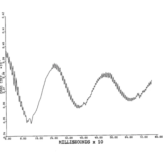
Figures 5.3 through 5.5 present time histories of the blade lift, drag, and moment normalized to the upstream dynamic pressure and the blade axial chord. Lift and drag are calculated in analogy with isolated airfoil theory, lift being defined as the component of force normal to the upstream flow direction, drag parallel to the upstream flow. Figure 5.6 shows the moment center on which Figure 5.5 is based. Several observations may be drawn from these figures, and are discussed in the following paragraphs.

The two frequency regimes are easy to see. The small ripples in these curves are due to the vortex shedding, which is superimposed upon a variation of much lower frequency.

The frequency and character of the vortex shedding are modulated by the low frequency variation. The shedding is strong during part of the low frequency cycle, i.e. its presence is easily seen in the overall blade force and moment. During the other part of the low frequency cycle, the shedding is weak being at times virtually undetectable in the overall force and moment. The strong shedding occurs at lower frequencies than the weak shedding. The total frequency range is approximately 11 KHz to 19 KHz.

The variation in vortex shedding strength is also evident in the convergence history plots. Figure 5.1 is a segment of the convergence history during which the shedding was strong. The periodicity is easy to see and measure. Figure 5.7 is a segment during which the shedding was weak. Periodicity is not obvious. The exact frequency of the weak shedding could not

always be determined.

The frequencies of the vortex shedding observed in the computation are in the range expected from Gertz's data presented in [3.2]. The shedding measured by Gertz was estimated to have a frequency f of approximately 15 KHz. The inlet relative Mach number at 60 percent span in his tests was about 1.17. The inlet relative Mach number in the computation is about 0.92. Assume that the shedding frequency is normalized by a length L and a velocity V. Assume also that the normalized shedding frequency fL/V is approximately the same for both experiment and computation, and that the length L is approximately the same in both cases. The expected shedding frequency for the computation would then be about 11.8 KHz. The average shedding frequency (total number of cycles divided by total time) observed in the computation is 13.8 KHz (17 percent greater than 11.8 KHz). This is considered to be good agreement given the approximate nature of the assumptions made above.

The lift, drag, and moment all vary significantly over the low frequency cycle. The total variation is defined as (maximum value - minimum value) / mean value. The total variation of lift is 5.21 percent, the total variation of drag is 13.13 percent, and the total variation of moment is 31.53 percent.

The flow variations due to the low frequency cycle are much greater than those due to the vortex shedding. Consider the blade moment for example. The largest variation in moment over one vortex shedding cycle is only about 1 percent of the time averaged moment. However, the largest variation due to the low frequency cycle is over 30 percent of the time averaged moment, as mentioned above. As will be discussed later, other gross flow field changes such as shock and separation point movement also occur at the low frequency; they are not seen to vary at the vortex shedding frequencies.

The large variations in blade forces due to the low frequency cycle are potentially important structural concerns. It happens that the frequency of these variations in the present computation (365 Hz) is near the real rotor's first bending frequency.

The low frequency variations of drag and moment appear to be in phase with one another, both lagging the lift by about 90 degrees.

The low frequency variations seem to be damping out. The decrease in the AC components is approximately exponential, the amplitude being multiplied by 1/e about every 4.7 milliseconds. This feature especially raises the question of whether these variations are mere numerical artifacts. The present investigation cannot answer this question conclusively. However, the nature of the low frequency cycle is worth studying seriously for several reasons.

(1) A mechanism whereby these fluctuations might be created by the numerical approximation is not evident at present. Several possibilities are considered in Chapter 7.

(2) A mechanism by which a real fluid dynamical cycle might be artificially damped by the numerical approximation is evident. The damping could be due to the effects of numerical smoothing over a large number of iterations. (Each low frequency cycle requires about 41000 iterations to complete.)

(3) The low frequency cycle is physically realistic. It is similar in many respects to cycles observed in transonic diffusers.

(4) The magnitude of these fluctuations is large enough to make them a significant factor in the design of transonic compressors if in fact they do represent a physical phenomenon.

the blade for two different times in the low frequency cycle. The "surface length" is defined as negative along the pressure surface (with the most negative value being the trailing edge), zero at the leading edge, and positive along the suction surface (ending again at the trailing edge). Recall that the blade surface is given an adiabatic (zero heat transfer) boundary condition in the work presented here. It is clear from Figure 5.8 that the temperature distributions necessary to support the adiabatic boundary condition would lead to significant heat transfer along the surface of the blade itself. In the shock regions, heat fluxes of 13 to 43 KW/mI would exist along the blade surface (taking the blade to be titanium with a thermal conductivity of 9 BTU/hr/ft/ 0F). The temperature distribution continually adjusts itself to maintain zero heat flux between the blade and the fluid. Such an adiabatic condition is very unlikely in a real unsteady flow. Perhaps a better approximate boundary condition is one in which the blade is assumed to have a high enough thermal inertia to maintain a constant temperature distribution. In this case, heat will be transferred from the flow to the blade and vice versa over the course of a time-varying flow cycle.

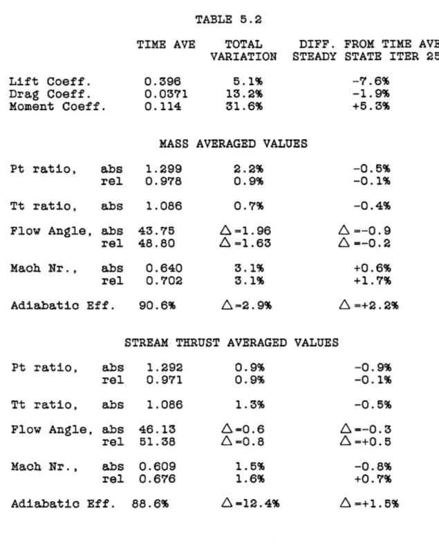
5.2 Comparison with Steady State Results

Table 5.1 presents the maximum range of unsteady values, the time averaged values, and values obtained from steady state iteration 2500 for a number of

quantities of interest.

Table 5.2 is a further analysis of the information presented in Table 5.1.

The total variations are calculated by dividing the difference between the maximum value and the minimum value by the time averaged value. For flow angles and efficiencies only the difference between the maximum and minimum values are tabulated (indicated by the symbol

A ).

subtracting the time averaged value from the steady state value and dividing by the time averaged value. Again, the symbol

A

It may be observed that the steady state solution significantly underpredicts the lift on the airfoil leading to a mild underprediction of the absolute total pressure ratio. It is also noteworthy that regardless of the averaging technique used, the steady state solution significantly overpredicts the adiabatic efficiency.

In this connection, it should be noted that the time-averaged efficiencies presented in Tables 5.1 and 5.2 have been obtained by using the time-averaged total pressure and total temperature ratios in the standard formula; they are not the result of time averaging all the instantaneous efficiencies. As Gertz has shown in [3.2], the instantaneous efficiency is not a good indication of the local instantaneous loss in an unsteady flow. The large difference between the time-averaged and steady state efficiencies is therefore the result of the seemingly small differences in the total temperature and total pressure ratios. The efficiency (and entropy change as well) is quite sensitive to small changes in these ratios, especially in the total temperature ratio, as demonstrated by the sample calculations presented in Table 5.3.

These comparisons have been made against steady state iteration 2500. Because of the lack of convergence, the steady state "solution" changes with the number of iterations. Somewhat different quantitative results would be obtained by examining different steady state solutions, but the qualitative character of the solution and its general relation to the time-accurate solutions is thought to be well represented by iteration 2500 discussed above.