Condition based monitoring and protection in electrical distribution systems

Condition Based Monitoring and Protection in

Electrical Distribution Systems

by

Uzoma Orji

B.S., Electrical Engineering

Massachusetts Institute of Technology (2006)

M.Eng., Electrical Engineering

Massachusetts Institute of Technology (2007)

ARCHWES

NA A SSAHSTS~S~

OF TECHFNOLOGY

ORARIFS

Submitted to the Department of Electrical Engineering and Computer

Science

in partial fulfillment of the requirements for the degree of

Doctor of Philosophy

at the

MASSACHUSETTS INSTITUTE OF TECHNOLOGY

February 2014

©

Massachusetts Institute of Technology 2014. All rights reserved.

Author ... . . ...

Departme

Electrical Engine i

and Computer Science

September 4, 2013

Certified by.

Steven B. Leeb

Professor of Electrical Engineering and Computer Science

Thesis Supervisor

A ccepted by

Leslie A. Kolodziejski

Chairman, Departmental Committee on Graduate Theses

Condition Based Monitoring and Protection in Electrical

Distribution Systems

by

Uzoma Orji

Submitted to the Department of Electrical Engineering and Computer Science on September 16, 2013, in partial fulfillment of the

requirements for the degree of Doctor of Philosophy

Abstract

The U.S. Department of Energy has identified "sensing and measurement" as one of the "five fundamental technologies" essential for driving the creation of a "Smart Grid". Consumers will need "simple, accessible..., rich, useful information" to help manage their electrical consumption without interference in their lives. There is a need for flexible, inexpensive metering technologies that can be deployed in many different monitoring scenarios. Individ-ual loads may be expected to compute information about their power consumption. New utility meters will need to communicate bidirectionally, and may need to compute param-eters of power flow not commonly assessed by most current mparam-eters. These mparam-eters may be called upon to perform not only energy score-keeping, but also assist with condition-based maintenance. They may potentially serve as part of the utility protection gear. And they may be called upon to operate in new environments, e.g., non-radial distribution systems as might be found on microgrids or warships. This thesis makes contributions in three areas of condition-based maintenance and protection in electric distribution systems.

First, this thesis presents a diagnostic tool for tracking non-integer harmonics on the utility. The tool employs a modified algorithm to enhance the capability of the Fast Fourier Transform (FFT) to determine the precise frequency of a newly detected harmonic. The efficacy of the tool is demonstrated with field applications detecting principal slot harmonics for speed estimation and diagnostics. Second, data from nonintrusive monitors have been shown to be valuable for power systems design. This thesis presents a new behavioral mod-eling framework developed for microgrid-style shipboard power system design using power observations from the ship's electrical distribution service. Metering can be used to inform new designs or update maintenance parameters on existing ship power systems. Finally, nonintrusive metering allows for new possibilities for adaptive fault protection. Adaptive thresholding of voltage magnitude, angle and harmonic content will be demonstrated for improving protection schemes currently used in ship electrical distribution systems. Thesis Supervisor: Steven B. Leeb

Acknowledgments

I wish to thank Professor Steven B. Leeb for his guidance and his advising. I am also thankful for the inputs from my thesis readers, Professors James L. Kirtley and Leslie K. Norford.

Thanks are due to the many colllaborators on this research: Warit Wichakool, Chris Schantz, Al-Thaddeus Avestruz, Jim Paris, Bartholomew Sievenpiper, Kather-ine Gerhard, Chad Tidd, Darrin Barber, Christopher Laughman, John Cooley, Zachary Remscrim, Shahriar Khushrushahi, Andrew Paquette, Ashley Fuller, Greg Elkins, Sabrina Neuman, Jeremy Leghorn, Zachary Clifford, Rachel Chaney, Daniel Vickery, John Donnal, Jin Moon, Mark Gillman, Kawin Surabitbovom, Niaja Farve, Arthur Chang, USCGC Escanaba Crew, Jukkrit Noppakunkajorn, and Andrew Carlson.

Finally, I wish to acknowledge the support I have received from my friends and family. Their words of encouragment are deeply appreciated.

This research was supported by the Office of Naval Research (ONR) Structural Acoustics Program led by program manager Debbie Nalchajian and the Grainger Foundation.

Contents

1 Introduction

1.1 Contributions . . . . 1.2 Organization . . . .

2 Nonintrusive Load Monitor (NILM) 2.1 Data Acquisition . . . . 2.2 Preprocessor Module . . . . 2.3 Event Detector Module . . . . 3 Speed Detection Using Slot Harmonics

3.1 Summary of Diagnostic Harmonics . . . 3.1.1 Air-Gap Eccentricity . . . . 3.1.2 Shaft-Speed Oscillation . . . . 3.1.3 Bearings Damage . . . . 3.2 Rotor Slot Harmonics . . . . 3.3 Practical Limitations on Slip . . . . 3.4 Speed Estimation via Slot Harmonics 3.5 Limitations to Proposed Method . 3.6 Airflow Diagnostics Application . . . . . 3.7 Reciprocating Compressors Application . 3.8 NilmDB and Cottage Street School . . . 3.9 Summary . . . . 26 27 28 29 30 32 32 35 . . . . 35 . . . . 36 . . . . 36 . . . . 37 . . . . 37 . . . . 40 . . . . 41 . . . . 50 . . . . 54 . . . . 57 . . . . 59 . . . . 61

4 Vibration Monitoring Using Shaft Speed Oscillation Harmonics

4.1 Current Method . . . . 64

4.2 Shaft Speed Oscillation Harmonics ... 65

4.3 Single Motor Environment ... ... 67

4.4 Multiple Motor Environment ... 70

4.4.1 No Previous Motor . . . . 71

4.4.2 _{Previous Motor . . . . 73}

4.4.3 _{Experiment . . . . 77}

4.4.4 Slip Difference . . . . 82

4.5 Effect of Fan Mounting Stiffness . . . . 84

4.6 _{Sum m ary . . . . 87}

5 Advanced Vibration Monitoring Using The Hilbert Transform 88 5.1 Background . . . . 88

5.2 Extracting Spectral Envelopes With The Hilbert Transform ... 90

5.3 Fan Vibration . . . . 92

5.3.1 Rotor Imbalance . . . . 92

5.3.2 Loose Mounting . . . . 97

5.4 Differentiating Source of Vibration . . . . 97

5.5 ESCANABA Data . . . 100

5.6 Sum m ary . . . 107

6 Behavioral Modeling Framework 108 6.1 Motivation and Background . . . 108

6.1.1 Why Focus on the DDG-51 Class? . . . . 111

6.1.2 DDG-51 Class Ship Introduction . . . . 112

6.2 Electric Plant Load Analysis (EPLA) . . . 115

6.2.1 Load Factor Analysis . . . . 115

6.2.2 Stochastic Load Analysis . . . 118

6.2.3 Modeling and Simulation . . . . 122

6.2.4 Potential Improvements . . . . 123 63

6.3 Sources of Information . . . . 6.3.1 Data Collection and Database Development . . 6.3.2 Machinery Control Message Acquisition System

6.3.3 USS SPRUANCE (DDG-111) Baseline Report

6.3.4 Nonintrusive Load Monitoring 6.4 Updating Existing Methods . . . .

6.4.1 Updating Load Factors . . . . 6.4.2 Updating Stochastic Load Analysis 6.5 Behavioral Modeling of DDG-51 Class . .

6.5.1 Introduction and Motivation . . . . 6.5.2 Ship Operational Concept . . . . . 6.5.3 Model Framework . . . . 6.5.4 Global Inputs . . . . 6.5.5 Modeling Ship System & Subsystem 6.5.6 Load Electrical Modeling . . . . 6.6 Stochastic Models . . . . 6.6.1 Constant . . . . 6.6.2 Uniform . . . . 6.6.3 Normal . . . . 6.6.4 Exponential . . . . 6.6.5 Goodness-of-Fit and Consistency 6.7 Behavioral Model Output and Results

6.7.1 Lighting Center . . . . 6.7.2 AC Plants . . . . 6.7.3 1SA . . . . 6.8 Conclusions and Future Work . . . . . . .

7 Multi-Function Monitor

7.1 Introduction . . . . 7.2 Integrated Protective Coordination System . . . .

Behaviors 124 125 126 127 128 129 130 145 150 151 153 155 158 159 166 172 173 173 173 175 176 178 178 180 182 184 187 187 189

7.2.1 System Information Matrix . . . .1 7.2.2 7.2.3 7.3 7.4 7.5 7.6 7.7 High Speed Relay Algorithm . Topology and Generator Line-7.2.4 Fault Type Determination . . Static Thresholds . . . . Nonintrusive Monitoring in Ring Powe High Impedance Faults . . . . Dynamic Thresholding . . . . Laboratory Experiments . . . . 7.7.1 Experiment I . . . . 7.7.2 Experiment II . . . . 7.7.3 Experiment III . . . . 7.7.4 Experiment IV . . . . 7.7.5 Experiment V . . . . 7.8 Conclusion . . . . . . . . 193 ip Assessment . . . 200 . . . 20 1 . . . 204 r Systems . . . 205 . . . . 207 . . . .. . . . 209 . . . ... . . . . 209 . . . .. . . . 212 . . . .. . . 215 . . . 218 . . . .. . . . .. . . 221 . . . .. . . . . .. . .. . . . . 224 .. . . . .. . . . 226 8 Conclusion and Future Work

A Derivation of Rotor Slot Harmonics A.1 Capacitor-Start Motors . . . . A.2 Capacitor-Run Motors . . . . A.3 Three-Phase Motors . . . . B Optimized Speed Estimation Method

B.1 getOptimalPSH.m . . . . B.2 getfft.m. . . . . . . . . . . . . . . . . Code . . . . . . . . C Vibration Monitoring Code

C.1 stiffnesseffect.m . . . .

D Hilbert Transform Spectral Envelope Code

D.1 getHilbertBands.m. . . . . 227 229 229 236 240 242 242 243 244 244 246 246 190

E Behavioral Modeling Framework Code E.1 mainGUI.m ... E.2 ShipSystem.m ... E.3 ShipComponent.m ... E.4 loadGloballnputs.m ... E.5 loadShipSystems.m ... E.6 loadSimulationParams.m ... E.7 loadPowerTraces.m ... E.8 loadLoadFactors.m ... E.9 mystrip.m ... E.10 carboncopy.m ... E.11 parseCell.m ... E.12 getRandomModelValue.m ... E.13 getOnTimes.m ... E.14 getTimeDependency.m ... E.15 getCurrentModel.m ... E.16 getTimeDependentPowerTrace.m . . . E.17 getFSMPowerTrace.m ... E.18 getSteadyStateVector.m ... E.19 getNormalSteadyState.m . . . . E.20 addTemperatureOffset.m ... E.21 checkModel.m ... E.22 evaluateRule.m ... F Dual-Generators Setup F. 1 Introduction ... F.1.1 Generators ...

F.1.2 Prime Movers (Engine) . . . . F.1.3 Power Supplies ...

F.1.4 Speed Encoder Mounts . . . .

248 . . . . 248 . . . . 258 . . . . 260 . . . . 264 . . . . 269 . . . . 272 . . . . 276 . . . . 279 . . . 283 . . . . 283 . . . . 283 . . . . 284 . . . . 284 . . . . 285 . . . . 286 . . . . 286 . . . . 286 . . . . 287 . . . . 288 . . . . 288 . . . . 289 . . . . 289 291 . . . . 291 . . . . 292 . . . . 293 . . . . 294 . . . . 294

F.1.5 Operational Limits of Generators . . . . F.2 Interfacing and Sensing . . . . F.2.1 Matlab Simulink® with The Real-Time Windows TargetT" F.2.2 PCI-4E-D PCI Interface Card ...

F.2.3 PCI-1710 Multifunction Cards . . . . F.2.4 SCSI Terminal Blocks ... ...

F.2.5 Current and Voltage Sensing ...

F.3 Remote Analog Programming of Power Supplies . . . . F.4 Front Panel F.4.1 Circuit Board . . . . F.5 S-Function Block . . . . F.5.1 Initialization . . . . F.5.2 Start . . . . F.5.3 Outputs . . . . F.5.4 Update . . . . F.5.5 Terminate . . . . F.6 System Identification . . . . F.6.1 One Frequency at a Time F.6.2 Matlab Controller Design F.6.3 Simulink Implementation. F.7 Overall Simulink Model . . . . F.8 Generator Performance... F.9 Conclusion . . . . G Dual Generators Simulink Code

G.1 sys..transferifunctionifinder.m . . . G.2 plant-controller_960PC14E.c... G.3 PlantController-Definitions.h . . . . G.4 PCL.1710_4EComm.c . . . . G.5 PCI4ESpeedFunctionDefinitions.h 295 295 295 296 297 298 298 300 301 302 302 303 303 304 305 305 305 306 310 311 318 318 321 323 323 324 338 339 347 . . . .

G .6 vectorm ath.c . . . . 348 G.7 Front Panel Circuit Board Schematic . . . . 350

List of Figures

2-1 A block diagram of the nonintrusive load monitor (NILM). ... 30 2-2 Schematic of the 60 Hz notch filter circuit. The circuit notches the

60 Hz frequency, amplifies the signal and sends the signal through an antialiasing filter. . . . . 31 2-3 Original nonintrusive transient classifier (NITC) block diagram. The

original NITC main program preprocesses, pattern matches and pro-duces output for three data queues. . . . . 33 2-4 Updated nonintrusive transient classifier (NITC) block diagram. This

version includes the filter and outputs the pre-trigger and post-trigger data. . . . . 34 3-1 Slot harmonics for a motor with the following parameters: f=60, k=1,

R=48, nd=0, s = 1.71% or 1180 rpm. The harmonics shown in the

figure are labeled with the corresponding value of v . . . . 39 3-2 _{Electrical current data stream with transient responses of induction}

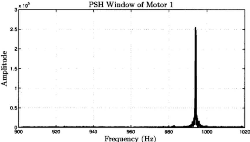
m achines. . . . . 42 3-3 The turn-on transient when Motor 1, labeled Region A in Fig. 3-2. . 42 3-4 Spectral envelope calculation. . . . . 43 3-5 FFT frequency content of the current between 900 Hz and 1020 Hz

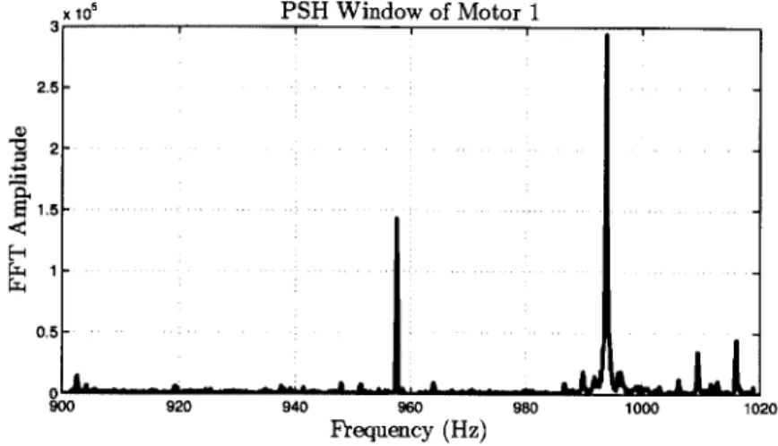
after Motor 1 has turned on and reached steady state. . . . 43 3-6 Current spectrum with with Motor 1 running. The frequency content

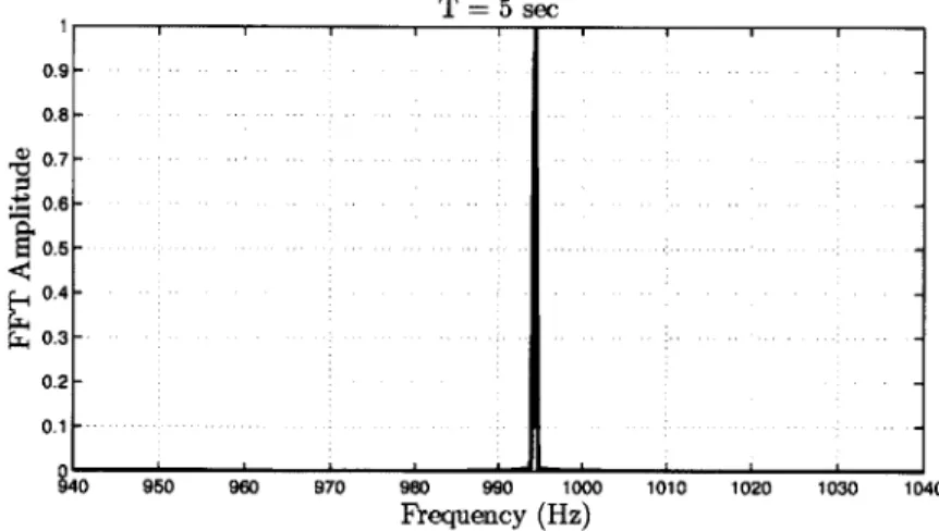
3-7 The FFT spectrum is shown for the sinusoid with a sampling time of

5 seconds. ... ... 44

3-8 The FFT spectrum is shown for a sinusoid with a frequency of 999.34 Hz with a sampling time of 0.5 seconds. As expected, the energy from the sinusoid is spread over multiple bins. . . . . 45 3-9 The FFT spectrum is shown for the sinusoid with a frequency of 999.34

Hz with a sampling time of 0.05 seconds. The frequency resolution is very coarse that a reliable speed estimate based on maximum value would be poor. . . . . 45 3-10 The observed PSH is shown in the solid line. The dotted line is the

FFT of the best-fit sinusoid. The sampling time is 0.5 seconds. ... 47 3-11 The observed PSH is shown in the solid line. The dotted line is the

FFT of the best-fit sinusoid. The sampling time is 0.05 seconds. . . . 47

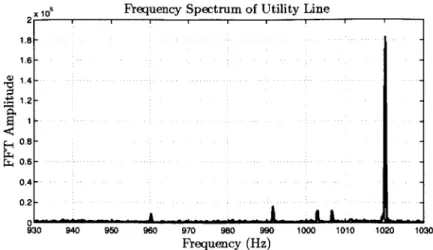
3-12 Frequency spectrum of the voltage from the utility line with inherent distortions. . . . . 49 3-13 The aggregate current spectrum in the PSH window of Motor 2 when

only Motor 1 is running. There are no noticeable features which should make the detection of the PSH of Motor 2 difficult. . . . . 49 3-14 The aggregate current spectrum in the PSH window of Motor 1 when

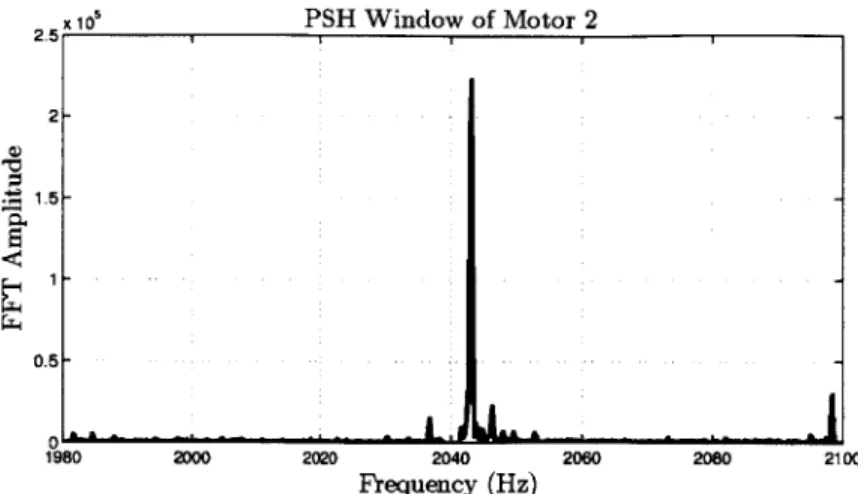
both motors are running. . . . . 50 3-15 The aggregate current spectrum in the PSH window of Motor 2 when

both motors are running. . . . . 51 3-16 Single housing used to enclose two ventilation fans. . . . . 52 3-17 Frequency content of the intake fan current. Its PSH is estimated to

be 2042.100 Hz and the speed is then estimated to be 3497.824 rpm. . 52 3-18 Frequency content of the exhaust fan current. Its PSH is estimated to

3-19 Frequency content of the current when both the intake and exhaust fans are on. The PSHs of both fans have shifted as the loading conditioning have changed. Comparing these PSHs to the PSHs when each motor

was turned on alone becomes challenging . . . . 53

3-20 Schematic diagram and picture of air handler unit. . . . . 55

3-21 Structure of the airflow estimation method . . . . 56

3-22 Illustration of airflow detectability using torque-speed curves that are generated from minimization against the motor current and the torque-speed curve, as collected for each blockage condition. . . . . 57

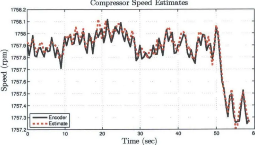
3-23 Speed estimate comparison of a compressor with a steady tank at 70 psi. The solid line is the estimate from the custom mounted encoder and the dotted line is the nonintrusive speed detection estimate. . . . 58

3-24 NILM Manager startup screen. . . . . 59

3-25 Cottage Street Elementary School in Sharon, MA . . . . 60

3-26 NILM install at the Cottage Street School . . . . 60

3-27 Raw current with ventilation fan turn on transient . . . . 60

3-28 Pre-trigger PSH window of ventilation fan . . . . 61

3-29 Post-trigger PSH window of ventilation fan . . . . 61

4-1 Simplified steady-state equivalent circuit model of motor containing only a voltage source and a slip-dependent rotor resistance. The lo-cation of the shaft speed oscillation harmonics can be determined by fully expressing the stator current i,(t). . . . . 65

4-2 Energy content for an HVAC evaporator fan for different amounts of weights. More weight leads to more vibration and more energy content in the shaft speed oscillation harmonic. . . . . 68

4-3 Shaft speed oscillation harmonic energy content for intake ventilation fan. More eccentric weight correlates with more energy content from the shaft speed oscillation harmonic. . . . . 69

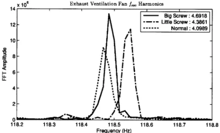
4-4 The shaft speed oscillation harmonic energy content for the exhaust ventilation fan is shown. . . . . 69 4-5 Harmonic content of a single phase, p = 1 ventilation fan near 118 Hz

is show n. . . . . 71 4-6 No harmonic content near 79 Hz. . . . . 72 4-7 Harmonic content of a single phase, p = 1 ventilation fan and a three

phase, p = 3 HVAC motor. The p = 1 ventilation fan has content near

118 H z. . . . . 72 4-8 The p = 3 HVAC fan has its harmonic near 79 Hz . . . . 72 4-9 The three phase, p = 3 HVAC fan has no harmonic content near 118

H z as shown. . . . . 73 4-10 No content near 79 Hz. . . . . 73 4-11 A plot of two sinusoids with frequencies 117.5 and 117.6 Hz with a

phase difference of < = r/7 is shown. . . . . 75 4-12 The sliding window algorithm shows the beat period of the energy

content. ... ... . ... .... .. .. . 76 4-13 Sliding window algorithm of 2 sinusoids with slips of .0412 and .0383.

With a larger absolute difference in slips between the 2 motors, the beat period has decreased. . . . . 77 4-14 When the intake ventilation fan runs by itself, its shaft speed oscillation

harmonic is shown. . . . . 78 4-15 The exhaust ventilation fan is then turned on and both oscillation

harmonics are shown. . . . . 78 4-16 The intake ventilation fan is then turned off and the oscillation

har-monic of the exhaust fan when running by itself is shown . . . . 79 4-17 The principal slot harmonics of the intake and exhaust ventilation fans

with an air filter placed over the intake fan. These harmonics can be used to estimate the speeds of each motor. . . . . 79

4-18 The bottom two traces show the sliding window algorithm results when the intake and exhaust ventilation fans are running by themselves. The top trace shows the sliding window when both fans are on. The harmonic energy content is periodic and the period can be determined from calculating the slips of each fan. . . . . 80 4-19 When the intake ventilation fan runs by itself with a higher slip, its

shaft speed oscillation harmonic is shown. . . . . 81 4-20 The exhaust ventilation fan is then turned on and both oscillation

harmonics are shown. . . . . 81 4-21 The intake ventilation fan is then turned off and the oscillation

har-monic of the exhaust fan when running by itself is shown. . . . . 81 4-22 The principal slot harmonics of the intake and exhaust ventilation fans

with cardboard placed over the intake fan. These harmonics can be used to estimate the speeds of each motor. . . . . 82 4-23 The bottom two traces show the sliding window algorithm results when

the intake and exhaust ventilation fans are running by themselves. The intake fan's airflow is blocked by a piece of cardboard. The top trace shows the sliding window when both fans are on. The harmonic energy content is periodic and the period can be determined from calculating the slips of each fan. . . . . 82 4-24 Duct fan picture . . . . 84 4-25 M odel of duct fan. . . . . 85 4-26 The effect of mounting stiffness on the electric detection metric. It can

be seen that the detection metric is sensitive to the vibration mounting stiffness. . . . . 86 5-1 Laboratory setup with two ventilation fans mounted to a steel frame. 93 5-2 A top view of the intake ventilation fan with no imbalance. . . . . 94 5-3 A screw attached to the fan hub imbalances the motor causing radial

5-4 Spectral content of the ventilation fan for five seconds of steady-state operation under baseline and faulty conditions between 50 and 60 Hz. All of the energy is centered around the frequency corresponding to the rotational speed of the fan. Approximating the energy in this frequency as a single sinusoid allows for the use of the Hilbert transform to easily track the envelope of the underlying sinusoid over time. . . . . 95 5-5 Acceleration levels in the 50 - 60 Hz frequency bands for three different

runs. The baseline test in which the fan has no imbalance gives the lowest amount of vibration. A second test was conducted with a screw added to the fan hub. The last test added a screw and a nut. The vibration levels increase accordingly. . . . . 96 5-6 An intake ventilation fan which is properly mounted to the steel frame. 97 5-7 An intake ventilation fan with loosened mounting screws. . . . . 98 5-8 The acceleration content in the 50-60 Hz frequency band for a

base-line test is shown. A second run was conducted in which the mounting screws are loosened. The acceleration content is also shown. As ex-pected, the readings show an increase in radial vibration. . . . . 98 5-9 Acceleration levels for the intake fan under normal ("baseline")

condi-tions, with a rotor imbalance ("screw"), and with a loose mount. The faulty runs both show an increase in vibration. However, this informa-tion alone is insufficient to differentiate the two flaws. More analysis is needed to diagnose the underlying fault. . . . . 99 5-10 Analysis of the 30-40 Hz frequency band is needed to differentiate

between a rotor imbalance of a loose mount. During turn-off transients, there is more energy in the sub-bands when there is a rotor imbalance. 100

5-11 USCG ESCANABA (WMEC-907). Measurements were taken from

two paired vacuum pumps located above the ship's engine room. . . . 101 5-12 Two vacuum pumps in the engine room on the ESCANABA. The motor

in the foreground will be referred to as Motor A. The motor in the background will be referred to as Motor B. . . . . 101

5-13 Raw acceleration of motor A when turned on. . . . 102

5-14 The acceleration content takes the raw data and computes the enve-lope of the Hilbert transform of the data between 50 and 60 Hz. The acceleration content metric can be computed by taking a region when the motor is in steady-state operation. . . . 102

5-15 Raw acceleration of motor A when motor B is turned on. The ampli-tude of the signals is greater than that in Fig. 5-13. . . . 103

5-16 The acceleration content is similar to that in Fig. 5-14. These metrics can be misleading if no further analysis is done. . . . 104

5-17 The raw acceleration of motor A when both motors A and B are turned on. Visual inspection of the time series shows that there is coupling be-tween the motors as there is a beat frequency present. This observation can be necessary in improving vibration diagnostics. . . . 105

5-18 Raw acceleration of motor A while the ship was at sea with visible acceleration from the rocking of the ship. . . . 106

5-19 The visible decoupled low-frequency rocking. . . . 106

5-20 The actual vibration from motor A. . . . 107

6-1 Electrical Load Growth on Surface Combatants. . . . 109

6-2 NGIPS Technology Development Roadmap . . . 110

6-3 Expected Inventory of Large Surface Combatants for Next 30 Years 111 6-4 ZEDS Electrical Distribution (Switchboards and MFMs Shown). . 114 6-5 Inter-relationship of DDS 310-1 Tasks. . . . 116

6-6 Uniform Distribution PDF and CDF. . . . 119

6-7 Triangular Distribution PDF and CDF. . . . 120

6-8 Discrete Distribution PDF and CDF. . . . 120

6-9 Monte Carlo Simulation Algorithm. . . . 121

6-10 Railgun Electrical Transient. . . . 123

6-11 NILM Power Trace of LBES 2A FOSP. . . . 129

6-33 6-34 6-35 6-36 6-37 6-38 6-39 6-40

Graphical Main Interface Screen . Global Inputs Menu . . . . AC System Relationships . . . . .

Model Ship System Entry . . . .

System Entry Selection Menu . Finite State Machine Example .

Fuel Service System Model . . . .

Load Modeling Selection Screen .

6-13 Fuel Oil Transfer Pump and Purifier Operation . . 6-14 Operation of Potable Water System . . . . 6-15 Fire and Seawater Service Pump Operating Profile 6-16 Detailed View of Fire Pump Switching Transient . 6-17 Fuel Service Pump Flow vs. Ship Speed . . . . 6-18 Shaft RPM vs. Ship Operating Speed . . . . 6-19 GTG At-Sea Operations . . . . 6-20 Comparison of Turbine Cooling Fans . . . . 6-21 Operation of Lube Oil Purifier . . . . 6-22 Operation of Purifier Heater . . . . 6-23 Individual AC Compressor Power Distributions . . 6-24 AC Compressor PDF . . . . 6-25 Average Cumulative Loading of all AC Plants . . . 6-26 Time Series of AC Plant Cumulative Load . . . . . 6-27 PDF of Lube Oil Purifier Heater Operation . . . . 6-28 ISA Loading Profile . . . . 6-29 CONOPS Mission Percentages for OPC. . . . . 6-30 CONOPS Speed-Time Profile for OPC. . . . . 6-31 Method of Creating Power Trace . . . . 6-32 DDG-51 Model Design Process . . . . .

6-41 Example Electrical Operating Data. . . . . 168 6-42 LBES Power Drawn by 2A FOSP During a FOSP Pump Shift Evolution. 170 132 133 134 134 138 139 141 143 144 145 147 147 148 148 150 152 154 155 156 157 160 161 161 162 162 164 165 167

6-43 AC Compressor Power Mean and Standard Deviation . . . 171

6-44 Total Ship Compressor Loading and Temperature Variation . . . 172

6-45 Electrical response of a fuel oil purifier . . . 174

6-46 Histogram of the steady-state region in the electrical response of a fuel oil purifier . . . 174

6-47 Example normal distribution for several values of N. Standard devia-tion decreases as N increases. . . . 177

6-48 Lighting center comparison . . . 179

6-49 Lighting center statistics . . . . 179

6-50 Time Series of AC Plant Cumulative Load . . . . 180

6-51 Model Results for single AC Compressor . . . 181

6-52 Comparison of AC Load Simulation and Actual Profile . . . 182

6-53 ISA Simulation (10 days) . . . 183

6-54 1SA Actual Load (10 Days) . . . 183

6-55 LBES Variation in MLO Pump With Maneuvering Transients. . . . . 186

7-1 DDG-51 Flight IIA ZEDS. This diagram includes the addressing, lo-cations and signal inputs of the MFMs. The defined positive direction of current flow is also shown for each MFM.. . . . 188

7-2 Functional Diagram of MFM. The diagram shows the sensor layout for the MFM. The three phase current and two voltage measurements per channel, the three ethernet communications channels and the shunt trip output to the associated circuit breaker. The shunt trip status input of the circuit breaker is not shown in the diagram. . . . . 189

7-3 Examples of Internal/Downstream Switchboard Faults. . . . 202

7-4 Possible Combinations For Bus-Tie Fault Scenarios. . . . 204

7-5 Example high impedance fault current from Texas A&M University. . 208 7-6 Example arcing current. . . . 208

7-7 Picture of the hardware model of a ship's ACZEDS. . . . . 210

7-9 Picture of the test MFM unit . . . . 211

7-10 Default topology and load configuration for laboratory experiments 211 7-11 Experiment I MFM channel currents . . . . 212

7-12 Total, real and reactive power spectral envelopes . . . . 213

7-13 Voltage distortion for the loads on the LC1B switchboard . . . . 214

7-14 Angle difference for the loads on the LC1B switchboard . . . . 214

7-15 Experiment II setup . . . . 215

7-16 Current drawn by the loads connected to the LC1B switchboard. . . . 216

7-17 Per unit voltage magnitude . . . . 216

7-18 Angle difference between voltage and Park's transformation rotating reference when L1 comes online . . . . 216

7-19 Absolute angle difference . . . . 217

7-20 Fundamental real power in both MFM channel for experiment II . . . 218

7-21 Experiment III setup . . . . 219

7-22 Current drawn by the loads connected to the LC1B switchboard. . . . 219

7-23 Per unit voltage magnitude . . . . 219

7-24 Angle difference between voltage and Park's transformation rotating reference when L1 comes online . . . . 220

7-25 Absolute angle difference . . . . 220

7-26 Fundamental real power in both MFM channel for experiment III . . 221

7-27 High impedance fault schematic . . . . 222

7-28 High impedance fault current . . . . 222

7-29 Experiment IV setup . . . . 222

7-30 Current drawn by the loads connected to the LC1B switchboard. . . . 223

7-31 Total power draw on LC1B switchboard . . . . 223

7-32 Angle difference for the loads on the LC1B switchboard for experiment IV . . . . 224

7-33 Shunt trip signal for MFM unit for experiment IV . . . . 224

7-34 Arcing fault schematic . . . . 224

7-36 Current drawn by the loads connected to the LC1B switchboard. . . . 225 7-37 Third harmonic content in the voltage for experiment V . . . 225 7-38 Shunt trip signal for MFM unit for experiment V . . . 226 A-1 Circuit diagram of a capacitor start motor. . . . 230 A-2 Cartoon sketch of an induction motor with concentrated winding and

the corresponding MMF wave. . . . 230 A-3 Circuit diagram of a capacitor run motor. . . . 237 F-1 Scaled hardware model of a shipboard electrical distribution system. . 291 F-2 Picture of the STC-5 generator. . . . 292 F-3 Coupled permanent magnet DC motors used as prime movers. . . . . 293 F-4 DC power supplies. 150 Vdc and 18 A and 2700 W . . . 294 F-5 Field Coil DC power supplies. 150 Vdc and 7 A and 1050 W . . . 294 F-6 Custom mount with shaft speed encoder. . . . 295 F-7 Interfacing and sensing layer . . . 296 F-8 Picture of the PCI-4E interface card. . . . 296 F-9 PCI-1710 multifunction card. . . . 297 F-10 SCSI terminal blocks are used to connect the PCI-1710 cards with

external components. . . . 298 F-11 Photograph of sense-box . . . 299 F-12 Schematics for the differential pair measurements for the voltages and

currents. . . . 301 F-13 Front panel user interface. . . . 301 F-14 Block diagram of overall system (or plant). . . . 306 F-15 Frequency response for the commanded voltage to monitored voltage.

The measured response is shown with the solid line. The low-order model is shown with the dotted line. . . . .. . . . 307 F-16 Frequency response for the monitored voltage to speed. The measured

response is shown with the solid line. The low-order model is shown with the dotted line. . . . 308

F-17 Frequency response for the commanded voltage to speed. The mea-sured response is shown with the solid line. The low-order model is shown with the dotted line. . . . . 309 F-18 Frequency response for the commanded voltage to field coil voltage.

The measured response is shown with the solid line. The low-order model is shown with the dotted line. . . . . 309 F-19 Overall block diagram of speed controller. . . . . 310 F-20 Inner frequency block within the speed controller. . . . . 312 F-21 Speed controller outer loop block. . . . . 314 F-22 Phase matching controller to parallel generators. . . . . 315 F-23 Inner block within the voltage controller. . . . . 316 F-24 Voltage controller outer loop block. . . . . 317 F-25 Overall Matlab Simulink model . . . . 319 F-26 Top plot shows the state of the parallel switch. The middle plot is the

state for the load switch. The bottom plot is the the angle difference between the voltages. . . . . 320 F-27 Angle difference between the voltages of the two generators. . . . . . 320 F-28 Speed of generators in response to a transient event. . . . . 321 F-29 Real power provided by each generator . . . . 322 F-30 Reactive power provided by each generator . . . . 322 G-1 Front panel circuit board schematic . . . . 351

List of Tables

3.1 _{Maximum Slip for Unambiguous Speed Estimation for Several Values} of R and p . . . . 41 3.2 _{Optimization Routine PSH and Speed Estimates at Different Sampling}

T im es . . . . 48 3.3 Differences in the location of the principal slot harmonics of the intake

and exhaust fans when the loading conditions change over time. . . . 54 3.4 PSH estimation for various lengths of times . . . . 61

4.1 This table lists the normalized energy content for different amount of weight added. This shaft speed oscillation harmonic energy correlates well with vibration reading from a vibration meter. . . . . 67 4.2 Vibration reading and energy content of intake and exhaust ventilation

fans under normal conditions, with a little screw and a big screw. More weight correlates with more vibration and more energy from the shaft speed oscillation harmonic. . . . . 69 4.3 Energy content of 2 sinusoids with various phase angle difference. The

harmonic content energy is a function of this phase difference. .... 74 4.4 Slip changes for the intake and exhaust ventilation fans. As shown, the

slip increases (speed decreases) for each motor when both are turned on. 83 4.5 _{This table shows the energy content of each fan when they are running}

by themselves. It also shows the error between the expected energy content when both are running and the observed. . . . . 83

5.1 Numerical energy levels in the second column for each of the tests con-ducted with the intake ventilation fan. These readings are consistent with those from a handheld vibration meter shown in the last column. 96 5.2 This table shows the numerical energy levels in the second column

for each of the tests conducted with the intake ventilation fan. These readings are consistent with those from a handheld vibration meter

shown in the last column. . . . . 98

6.1 DDG-51 Class Basic Characteristics . . . . 112 6.2 Load Factor Analysis Calculation . . . . 118 6.3 DDGs Visited for Data Analysis . . . . 125 6.4 MCMAS Derived Load Utilization Rates . . . . 136 6.5 Operating Mode Determination of GTM Utilization . . . . 137 6.6 Summary of Load Utilization for Selected Propulsion Components . . 142 6.7 Lube Oil Purification Load Factor . . . . 145 6.8 Ship-Type Definitions of a DDG-51 . . . . 157

7.1 MFM III address/number/location/type assignment . . . . 190 7.2 Possible values of the fault status output of the HSR routine . . . . . 196 7.3 Generator line-up for each possible state . . . . 201 7.4 Thresholds for the IPCS routine . . . . 205 7.5 Loads used in laboratory experiments . . . . 212

F.1 Nameplate data of the STC-5 generator. . . . . 292 F.2 Nameplate data of the permanent magnet DC motors. . . . . 293

Chapter 1

Introduction

When the U.S. Department of Energy identified "sensing and measurement" as one of the "five fundamental technologies" essential for driving the creation of a "Smart Grid", one of the goals included a "deployment of 'smart' technologies ... for meter-ing, communications concerning grid operations and status, and distribution automa-tion." Other goals included "integration of 'smart' appliances and consumer devices" and "development and incorporation of demand response, demand-side resources, and energy-efficiency resources" [1]. The Smart Grid would require "smart" metering de-vices and communication networks to collect and deliver necessary information about the power system for the operation of the power grid to the consumer. Consumers

will need quick, easy access to "simple, accessible ... , rich, useful information" to help manage their electrical consumption without interference in their lives.

There is also a need for flexible, inexpensive metering technologies that can be deployed in many different monitoring scenarios. Such smart devices should be able to provide not only just the total power consumed but could also give diagnostic pa-rameters of loads from the electrical signals. Diagnostic papa-rameters such as the rotor speed of an induction motor and high frequency variation of the power consumption can be extracted by smart meters to provide additional information about the health of these loads.

As these demands become apparent for a smarter grid, new technologies will be needed for efficient control and access to power systems. These include the need for

diagnostic systems to track pathological energy consumption, new design techniques for smaller or "islanded" power systems and new protection schemes. This thesis looks to make contributions in these areas.

1.1

Contributions

Extensive research has been in condition based monitoring by tracking speed, vi-bration, temperature, pressure and other metrics to monitor monitor faults such as broken rotors bars, damaged bearings, rotor eccentricity and shaft speed oscillations. These methods are not only limited for single loads but also may require intrusive installation of external sensors. This thesis will develop methods to track harmonics using power measurements from electrical signals in single loads and will also extend these methods for multiple loads.

Second, data from nonintrusive monitors have been shown to be valuable for power systems design. This thesis presents a new behavioral modeling framework developed for microgrid-style shipboard power system that improves upon existing methods. The framework makes use of using power observations from the ship's electrical distribution service to develop stochastic models used in simulating the total load of a ship. Metering can be used to inform new designs or update maintenance parameters on existing ship power systems.

Finally, nonintrusive metering allows for new possibilities for adaptive fault pro-tection in zonal electrical distributions. Current methods use static threshold levels for fault detection which may be insufficient depending on type of fault or operating condition. This thesis presents an adaptive fault detection which uses the data from nonintrusive for improved fault detection. Adaptive thresholding of voltage mag-nitude, angle and harmonic content will be demonstrated for improving protection schemes currently used in ship electrical distribution systems.

1.2

Organization

A background information on previous work on nonintrusive load monitoring (NILM) is presented in Chapter 2. Hardware improvements were made to NILM to allow for tracking of small harmonics in the electrical signals used for condition-based mainte-nance (CBM) through electrical monitoring.

Chapters 3 and 4 present methods for estimating speed and vibration by tracking harmonics in the electrical signals for loads. Experiments and results are presented to show the results of the methods. The NILM environment allows for CBM for multiple loads as will be explained. Chapter 5 discusses CBM for vibration using acceleration when tracking harmonics in the electrical signals becomes infeasible.

Chapter 6 describes the framework that can be used for future ship for improved reliability of electric distribution systems. A software graphical user interface (GUI) is shown to implement the design of the framework.

Chapter F presents a testbench shipboard dual-generator setup and Chapter 7 describes the implementation of a multi-function monitor in the protection of a test-bench MVAC zonal electrical distribution system. Computer simulation is used to shown the efficacy of the improved algorithm for zonal protection.

Chapter 2

Nonintrusive Load Monitor

(NILM)

The nonintrusive load monitor has been demonstrated [2-5] as an effective tool for evaluating and monitoring electro-mechanical systems through analysis of electrical power data. The power distribution network can be pressed into "dual-use" service, providing not only power distribution but also a diagnostic monitoring capability based on observations of the way in which loads draw power from the distribution service. A key advantage of the nonintrusive approach is the ability to reduce sensor count by monitoring a collections of loads. A pictorial representation of the NILM is shown in Fig. 2-1

Nonintrusive electrical monitoring has been described in [7, 8] and in other pub-lications. The systems that are described in these papers can be split into two broad categories: transient and steady-state approaches. The transient approach [8] finds loads by examining the full detail of their transient behavior. Reference [2] describes a platform for transient-based nonintrusive load monitoring appropriate for many ap-plications. The following sections will discuss the data acquisition, preprocessor and

voltagecurrent

measurementsl measurements

Control inputs

Outputs Status Reports

Fig. 2-1: A block diagram of the nonintrusive load monitor (NILM) [6].

2.1

Data Acquisition

NILM experiments from previous research collect data from a current sensor with only analog filtering for anti-aliasing. There is a large 60 Hz line frequency component that dominates the current signal, making detection of the smaller harmonics in the current discussed in chapters 3 and 4 more difficult. To improve the detectability of the harmonics, a 60 Hz notch filter is implemented to remove the large line frequency component before the data acquisition hardware in the NILM samples the current.

In Fig. 2-2, the stator current signal is sent through a 60 Hz notch filter. The output is amplified by a gain stage and later filtered by a passive antialiasing filter. The output buffer drives the input of the NILM data acquisition hardware. The notch filter stage allows for improved signal detectability of the smaller slot harmonics. By removing the large dominant line frequency, the smaller harmonic signals can then be amplified, increasing the overall signal-to-noise ratio by reducing the effect of quantization noise in the analog-to-digital converter (ADC) of the NILM.

12

I

VlM

A

T

_Box

Fig. 2-2: Schematic of the 60 Hz notch filter circuit. The circuit notches the 60 Hz frequency, amplifies the signal and sends the signal through an antialiasing filter.

50k 50k 100pF 1O88pF 50k 50k UAF42 50k 50k 1008pF 10 8pF ++ 50k 50k UAF42

2.2

Preprocessor Module

The NILM detects the operation of individual loads in an aggregate power measure-ment by preprocessing measured current and voltage waveforms to compute spectral envelopes [9]. Spectral envelopes are short-time averages of the line-locked harmonic content of a signal. For an input signal x(t) of current, the in-phase spectral envelopes

ak of x are

2 ~

ak(t) = - x(r) sin(kw-)cd-, (2.1)

T _{_t-T}

where k is the harmonic index. The quadrature spectral envelopes bk are

2 pt

bk(t) = - x(-r) cos(kw-r)dT. (2.2)

T tT

These spectral envelopes may be recognized as the coefficients of a time-varying Fourier series of the input waveform. For transient event detection on the ac util-ity, the time reference is locked to the line so that fundamental frequency spectral envelopes correspond to real and reactive power in steady state. Higher spectral envelopes correspond to line frequency harmonic content. A high performance tran-sient event detection algorithm [8, 10] is available to disaggregate the fingerprints or spectral envelope signatures of individual loads in the aggregate measurement. This transient event detection is critical for pre-trigger and post-trigger event detection described in §2.3.

2.3

Event Detector Module

By computing line-locked spectral envelopes from input signals, NILM can detect the activation of a motor of interest. Special attention can then be paid to the aggregate current frequency content just before and just after this turn-on transient, as will be shown in Chapters 3 and 4, to identify important frequency content that occurs at frequencies that are not line-locked.

in block diagram form in Fig. 2-3. The relevant parts of the NITC routine are slightly modified for the purposes of this thesis.

v(t) i (t)

Data Collection Hardware

VnI V pin Preprocessing raw envelop Pattern Matching tag data Text es envelope, tag and match data

tag, envelope and raw

Diagnostics

I

Graphics

Fig. 2-3: Original nonintrusive transient classifier (NITC) block diagram. The original NITC main program preprocesses, pattern matches and produces output for three data queues [9].

The updated NITC block diagram is shown in Fig. 2-4.

v(t) i(t)

Notch Filter

Data Collection Hardware

_ IF I__ "I

Transient Event Detector

1

7

pre-trigger post-trigger

Fig. 2-4: Updated nonintrusive transient classifier (NITC) block diagram. This ver-sion includes the filter and outputs the pre-trigger and post-trigger data.

Once the unfiltered data has been collected by the hardware, the data is prepro-cessed to produced the spectral envelopes. The pattern matching routine identifies a trigger event once a motor has turned on. The outputs of this pattern matching routine are now the filtered raw data before and after this trigger event. Once the

pre-trigger and post-trigger data are saved, they can be used to identify frequency

Chapter 3

Speed Detection Using Slot

Harmonics

Harmonic analysis of motor current has been used to track the speed of motors for sensorless control. Algorithms exist that track the speed of a motor given a dedicated stator current measurement, for example [11-15]. Harmonic analysis has also been applied for diagnostic detection of electro-mechanical faults such as damaged bearings and rotor eccentricity [16-27].

Rotor slot harmonics are widely used in nonintrusive speed detection algorithms used in many control applications. The ability to estimate the speed of an electric machine from its electrical signals provides a method that does not require the instal-lation and maintenance of sensors or any other hardware. This chapter discusses the limitations of previous research that use these rotor slot harmonics for speed tracking. The improved method developed in this research provides a routine that can estimate the speed with a reduced number of line cycles for faster updates. This chapter con-cludes with examples that require speed estimation for various applications.

3.1

Summary of Diagnostic Harmonics

Induction motors are vital components of many industrial processes. Extensive re-search is being done to develop techniques to monitor these motors to minimize the

risk of unexpected system failures and reduced motor lifetime. Generally, condition monitoring algorithms have focused on the stator, the rotor or the bearings for sens-ing certain failures. Most of the recent research is now focused on the electrical monitoring of the stator current spectrum of the motor to sense various faults [16] as discussed below.

3.1.1

Air-Gap Eccentricity

Two methods have been proposed for detecting air-gap eccentricity. Reference [26] monitors the sideband frequencies of slot harmonics located at

=S1ot+eCC = f [(kR

+

where

f

0, ±1,... is the order of rotor eccentricity; s is the per unit slip, S is the speed in rotations per minute (rpm), p is the number of pole pairs and v =_ ±, I3, ... is the stator MMF harmonic order [15, 28]. For specific values of k, nd and v, the corresponding slot harmonics can be used to track speed of the induction motor. A speed detection scheme using these harmonics is discussed later in this chapter.

The second method, used in [18], searches for fundamental sidebands of the supply frequency. These eccentricity harmonics are located at

fecc

=

f

where m = 1,2,3,....

3.1.2

Shaft-Speed Oscillation

Shaft-speed oscillation is a mechanical fault that can be enhanced by certain rotor imbalances. An improperly mounted motor or an unbalanced fan can accentuate

shaft-speed oscillation frequencies [18]. The frequencies of interest are predicted by

f

f

Chapter 4 discusses how the shaft-speed oscillation harmonics can be used for vibra-tion analysis.

3.1.3

Bearings Damage

Misalignment of the bearings can produce physical damage of the raceways which house the bearings. The resulting mechanical displacement causes the air gap to vary and the eccentricity harmonics are located at the following frequencies given by

fAng -f ±M I ,, (3.4)

where m = 1,2, 3, ... and

fi,O

io = nfr 1 ± cos , (3.5)

2 pd

where n is the number of bearing balls, fr is the mechanical rotor speed in rotations per second, bd is the ball diameter, pd is the bearing pitch diameter, and 3 is the contact angle of the balls in the raceway [22].

This thesis does not explore diagnostics using these bearings frequencies. The following section discusses the slot harmonics derived from (3.1).

3.2

Rotor Slot Harmonics

Rotor slot harmonics present in the stator current of a motor arise from the inter-action between the permeance of the machine and the magnetomotive force (MMF) of the current in the stator windings. As the motor turns, the rotor slots alter the

effective length of the airgap sinusoidally, thereby affecting the permeance of the ma-chine. This sinusoidal behavior is seen in the flux, which is the product of the MMF and the permeance across the airgap. The odd harmonics present in the stator cur-rent introduce additional harmonics. Static and dynamic eccentricity harmonics also appear in the stator current as the rotor turns irregularly in relation to the stator.

The slot harmonics, including the principal slot harmonic (PSH), are located at frequencies

fh = f R +V =f R +v , (3.6)

p . 3600 _

where f is the supply frequency; R is number of rotor slots; s is the per unit slip,

S is the speed in rotations per minute (rpm), p is the number of pole pairs and

v = i1, ±3, ... _{is the stator MMF harmonic order [15, 28]. These harmonics are}

located in the family of harmonics given by (3.1) for k = 1 and nd = 0. For the data presented in this thesis, there was little rotor imbalance so the most visible slot harmonics are given by (3.6).

When the locations of these speed-dependent harmonics are found, the speed of the electric machine can be calculated rather easily. A full discussion on how these speed-dependent harmonics appear in the stator current can be found in Appendix A.

A substantial amount of literature makes use of (3.6) for speed detection [11-13, 15, 29, 30]. To illustrate, the frequency spectrum of 5 seconds of current from a motor with its slot harmonics (3.6) is shown in Fig. 3-1 for different values of v. The motor used was a three-phase machine with R = 48 rotor slots and p = 3 pole pairs loaded by a dynomometer to run at s = 0.0171 or 1180 rpm. Typically, the slot

harmonics with k = _{1, referring to the fundamental harmonic of the stator current,}

and with nd = 0, referring to the case in which the motor has no eccentricity, are

the most pronounced in the current spectrum [11, 31]. The PSH corresponds to the harmonic with v = 1. For a given nd, the slot harmonics differ exactly by 2f in (3.6).

4. 3. 2. 0. 750 800 850 900 950 1000 1050 1100 1150 Frequency (Hz)

Fig. 3-1: Slot harmonics for a motor with the following parameters: f=60, k=1,

R=48, nd=0, s = 1.71% or 1180 rpm. The harmonics shown in the figure are labeled

with the corresponding value of v.

performance of these approaches can be limited in terms of accuracy, linearity, res-olution, speed range, or speed of response [14]. Any analog filtering can require extremely complex circuitry and any output signal can be corrupted by noise. Dig-ital techniques employing the Fast Fourier Transform (FFT) were developed [12] to overcome the flaws in the analog methods. These FFT methods were limited by the uncertainty principle, i.e. the trade-off between high frequency resolution and the response time to changes of speed that deteriorates with long data records. Para-metric estimations [11, 13, 15] of the current spectrum were used to overcome the limitations of FFT by attempting to model the process that samples the data using

a priori knowledge. However, these estimations require digital filters which make

these methods less robust than the FFT. With a high stator frequency, the longer computations times can reduce any advantage these parametric methods may have over the FFT.

Some research has been done to combine the FFT and parametric estimation methods [11, 15]. In [11], the techniques do a successful job in tracking the slot harmonics in estimating speeds in a controlled environment. The authors make use of the periodicity of the slot harmonics by aliasing the spectrum such that these harmonics line up to increase detectability.

There are certain trade-offs that must be made when deciding on the proper

< 10 01t armonics 5 4-5 - . 3 -5= 2-51

1

JL1

J-

methods for detecting these speed-dependent rotor slot harmonics. The choices are often dictated by the practical setting. In the experiments conducted in this research, it is observed that the principal slot harmonic (PSH) is the most pronounced slot harmonic in the motors. The methods discussed here, therefore, will only search for the PSH, which simplifies the complexity of the algorithm unless otherwise specified. Furthermore, the method combines the powers of the FFT and a search routine to find the best estimate for the true location of the PSH. Moreover, previous work could only estimate the speed of a single motor [11-15]. This method can estimate speed of multiple motors in a multi-motor environment. A full discussion follows below.

3.3

Practical Limitations on Slip

For high-efficiency induction motors, the slip s usually does not exceed 5% and pos-sibly less. This assumption leads to interesting simplifications when searching for the principal slot harmonic (PSH). The PSH refers to the slot harmonic with v = 1,

k = 1, and nd= _{0 in (3.6) and is used in speed detection algorithms since it is often}

the most pronounced [11, 31]. The slot harmonics for different values of v differ by 2f = 120 Hz. If the principal slot harmonic was confined to a frequency window of width 120 Hz under these practical limitations of slip, there would be no ambiguity

in determining the window in which the PSH is located.

For example, Table 3.1 tabulates the maximum slip for different values of R and p for which the PSH would be confined to a 120 Hz wide frequency window. For a motor with R = _{60 and p = 1, a maximum slip of s = 0.033 would need to be}

assumed in order to constrain the PSH to a 120 Hz wide window. This assumption would be unreasonable because it would be possible for the motor to be running with a slip of 0.04. In this situation, there would be some ambiguity in determining in which window the PSH lies.

On the other hand, a motor with R = 48 and p = 3 can have a maximum slip of s = 0.125 to unambiguously determine the window of the PSH. If the motor were running with no slip (s = 0), the principal slot harmonic would be located at 1020 Hz.

Table 3.1: Maximum Slip for Unambiguous Speed Estimation for Several Values of R and p p R 1 2 3 4 16 0.1247 0.2494 0.3742 0.4989 20 0.0997 0.2000 0.3000 0.4000 24 0.0833 0.1667 0.2492 0.3333 28 0.0714 0.1428 0.2142 0.2856 32 0.0622 0.1244 0.1875 0.2489 34 0.0586 0.1172 0.1758 0.2344 40 0.0500 0.1000 0.1500 0.1989 44 0.0453 0.0906 0.1358 0.1811 48 0.0417 0.0833 0.1250 0.1667 52 0.0383 0.0767 0.1150 0.1533 56 0.0356 0.0711 0.1067 0.1422 60 0.0333 0.0667 0.1000 0.1333

If the motor were running with slip (s = 0.125), the principal slot harmonic would be located at 900 Hz. Therefore, it can be assumed that the principal slot harmonic will be located in the 120 Hz window between 900 Hz and 1020 Hz. This slip satisfies any reasonable low-slip assumptions.

3.4

Speed Estimation via Slot Harmonics

Using a "low-slip" assumption in which the PSH is restricted to a single 120 Hz wide frequency window, this section will describe the application of the slot harmonics in determining speed of operation just after startup in a multi-load/multi-motor envi-ronment. All Matlab code for this optimized speed estimation method is shown in

Appendix B. To demonstrate the effectiveness of the algorithm, the speed estimation method was conducted with the following two motors. The first motor (Motor 1) was a three-phase motor from an HVAC evaporator in an air-handling unit. Motor 1 had R = 48 rotor slots and p = 3 pole pairs. The second motor (Motor 2) is a single-phase line-to-line machine from a fresh-air ventilation unit with R = 34 rotor slots and p = 1 pole pairs.