HAL Id: hal-01181205
https://hal.inria.fr/hal-01181205
Submitted on 30 Jul 2015
HAL is a multi-disciplinary open access
archive for the deposit and dissemination of
sci-entific research documents, whether they are
pub-lished or not. The documents may come from
teaching and research institutions in France or
abroad, or from public or private research centers.
L’archive ouverte pluridisciplinaire HAL, est
destinée au dépôt et à la diffusion de documents
scientifiques de niveau recherche, publiés ou non,
émanant des établissements d’enseignement et de
recherche français ou étrangers, des laboratoires
publics ou privés.
Copyright
A Network-Aware Approach for Searching As-You-Type
in Social Media
Paul Lagrée, Bogdan Cautis, Hossein Vahabi
To cite this version:
Paul Lagrée, Bogdan Cautis, Hossein Vahabi. A Network-Aware Approach for Searching As-You-Type
in Social Media. 24th ACM International Conference on Information and Knowledge Management
-CIKM 2015, Oct 2015, Melbourne, Australia. �hal-01181205�
A Network-Aware Approach for Searching
As-You-Type in Social Media
Paul Lagrée
Inria Saclay and UniversitéParis-Sud Orsay, France
[email protected]
Bogdan Cautis
Inria Saclay and UniversitéParis-Sud Orsay, France
[email protected]
Hossein Vahabi
Yahoo Labs Barcelona, Spain[email protected]
ABSTRACT
We present in this paper a novel approach for as-you-type top-k keyword search over social media. We adopt a natural “network-aware” interpretation for information relevance, by which informa-tion produced by users who are closer to the seeker is considered more relevant. In practice, this query model poses new challenges for effectiveness and efficiency in online search, even when a com-plete query is given as input in one keystroke. This is mainly be-cause it requires a joint exploration of the social space and classic IR indexes such as inverted lists. We describe a memory-efficient and incremental prefix-based retrieval algorithm, which also ex-hibits an anytime behavior, allowing to output the most likely an-swer within any chosen running-time limit. We evaluate it through extensive experiments for several applications and search scenar-ios, including searching for posts in micro-blogging (Twitter and Tumblr), as well as searching for businesses based on reviews in Yelp. They show that our solution is effective in answering real-time as-you-type searches over social media.
Categories and Subject Descriptors
H.3.3 [Information Search and Retrieval]General Terms
Algorithms, Theory
Keywords
As-you-type search; network-aware search; social networks; mi-croblogging applications.
1.
INTRODUCTION
Information access on the Web, and in particular on the social Web, is, by and large, based on top-k keyword search. While we witnessed significant improvements on how to answer keyword queries on the Web in the most effective way (e.g., by exploiting the Web structure, user and contextual models, user feedback, se-mantics, etc), answering information needs in social applications requires often a significant departure from socially-agnostic ap-proaches, which generally assume that the data being queried is decoupled from the users querying it. The rationale is that social links can be exploited in order to obtain more relevant results, valid not only with respect to the queried keywords but also with respect to the social context of the user who issued them.
While progress has been made in recent years to support this novel, social and network-aware, query paradigm – especially to-wards efficiency and scalability – more remains to be done in order
to address information needs in real applications. In particular, pro-viding the most accurate answers while the user is typing her query, almost instantaneously, can be extremely beneficial, in order to en-hance the user experience and to guide the retrieval process.
In this paper, we adapt and extend to the as-you-type search sce-nario – one by now supported in most search applications, includ-ing Web search – existinclud-ing algorithms for top-k retrieval over so-cial data. Our solution, called TOPKS-ASYT (for TOP-k Soso-cial- Social-aware search AS-You-Type), builds on the generic network-Social-aware search approach of [21, 25] and deals with three systemic changes: 1. Prefix matching: answers must be computed following a query interpretation by which the last term in the query se-quence can match tag / keyword prefixes.
2. Incremental computation: answers must be computed in-crementally, instead of starting a computation from scratch. For a query representing a sequence of terms (keywords) Q = [t1, . . . , tr], we can follow an approach that exploits what has already been computed in the query session so far, i.e., for the query Q0 = [t1, . . . , tr−1, t0r], with t
0
rbeing a
one character shorter prefix of the term tr.
3. Anytime output: answers, albeit approximate, must be ready to be outputted at any time, and in particular after any given time lapse (e.g., 50 − 100ms is generally accepted as a rea-sonable latency for as-you-type search).
We consider a generic setting common to a plethora of social ap-plications, where users produce unstructured content (keywords) in relation to items, an activity we simply refer to as social tagging. More precisely, our core application data can be modelled as fol-lows: (i) users form a social network, which may represent relation-ships such as similarity, friendship, following, etc, (ii) items from a public pool of items (e.g., posts, tweets, videos, URLs, news, or even users) are “tagged” by users with keywords, through various interactions and data publishing scenarios, and (iii) users search for some k most relevant items by keywords.
We devise a novel index structure for TOPKS-ASYT, denoted CT-IL, which is a combination of tries and inverted lists. While basic trie structures have been used in as-you-type search scenarios in the literature (e.g., see [18] and the references therein), ranked access over inverted lists requires an approach that performs ranked completion more efficiently. Therefore, we rely on a trie structure tailored for the problem at hand, offering a good space-time trade-off, namely the completion trie of [11], which is an adaptation of the well-known Patricia trie using priority queues. This data struc-ture is used as the access layer over the inverted lists, allowing us to read in sorted order of relevance the possible keyword comple-tions and the items for which they occur. Importantly, we use the completion trie not only as an index component over the database,
but also as a key internal component of our algorithm, in order to speed-up the incremental computation of results.
In this as-you-type search setting, it is necessary to serve in a short (fixed) lapse of time, with each keystroke and in social-aware manner, top-k results matching the query in its current form, i.e., the terms t1, . . . , tr−1, and all possible completions of the term tr. This must be ensured independently of the execution configu-ration, data features, or scale. This is why we ensure that our al-gorithms have also an anytime behaviour, being able to output the most likely result based on all the preliminary information obtained until a given time limit for the TOPKS-ASYT run is reached.
Our algorithmic solution is validated by extensive experiments for effectiveness, feasibility, and scalability. Based on data from the Twitter and Tumblr micro-blogging platforms, two of the most popular social applications today, we illustrate the usefulness of our techniques for keyword search for microblogs. Based on reviews from Yelp, we also experiment with keyword search for businesses. The paper is organised as follows. In Section 2 we discuss the main related works. We lay out our data and query model in Sec-tion 3. Our technical contribuSec-tion is described in SecSec-tion 4 and is evaluated experimentally in Section 5. We conclude and discuss follow-up research in Section 6. For space reasons, more experi-ments and discussions can be found in a technical report [15].
2.
RELATED WORK
Top-k retrieval algorithms, such as the Threshold Algorithm (TA) and the No Random Access algorithm (NRA) [8], which are early-termination, have been adapted to network-aware query mod-els for social applications, following the idea of biasing results by the social links, first in [31, 25], and then in [21] (for more de-tails on personalized search in social media we refer the interested readers to the references within [21, 25]).
As-you-type (or typeahead) search and query auto-completion are two of the most important features in search engines today, and could be seen as facets of the same paradigm: providing accurate feedback to queries on-the-fly, i.e., as they are being typed (possi-bly with each keystroke). In as-you-type search, feedback comes in the form of the most relevant answers for the query typed so far, allowing some terms (usually, the last one in the query sequence) to be prefix-matched. In query auto-completion, a list of the most rel-evant query candidates is to be shown for selection, possibly with results for them. We discuss each of these directions separately.
The problem we study in this paper, namely top-k as-you-type search for multiple keywords, has been considered recently in [18], in the absence of a social dimension of the data. There, the authors consider various adaptations of the well-known TA/NRA top-k al-gorithms of [8], even in the presence of minor typing errors (fuzzy search), based on standard tries. A similar fuzzy interpretation for full-text search was followed in [12], yet not in a top-k setting. The techniques of [17] rely on precomputed materialisation of top-k re-sults, for values of k known in advance. In [2, 3], the goal is finding all the query completions leading to results as well as listing these results, based on inverted list and suffix array adaptations; however, the search requires a full computation and then ranking of the re-sults. For structured data instead of full text, type-ahead search has been considered in [9] (XML) and in [16] (relational data).
Query auto-completion is the second main direction for instant response to queries in the typing, by which some top query comple-tions are presented to the user (see for example [27, 26, 4] and the references therein). This is done either by following a predictive approach, or by pre-computing completion candidates and storing them in trie structures. Probably the best known example today is the one of Google’s instant search, which provides both query
pre-dictions (in the search box) and results for the top prediction. Query suggestion goes one step further by proposing alternative queries, which are not necessarily completions of the input one (see for in-stance [29, 13]). In comparison, our work does not focus on queries as first-class citizens, but on instant results to incomplete queries.
Person (or people) search represents another facet of “social search”, related to this paper, as the task of finding highly relevant persons for a given seeker and keywords. Usually, the approach used in this type of application is to identify the most relevant users, and then to filter them by the query keywords [24, 1]. In this area, [6] describes the main aspects of the Unicorn system for search over the Facebook graph, including a typeahead feature for user search. A similar search problem, finding a sub-graph of the social network that connects two or more persons, is considered under the instant search paradigm in [30].
Several space-efficient trie data structures for ranked (top-k) completion have been studied recently in [11], offering various space-time tradeoffs, and we rely in this paper on one of them, namely the completion trie. In the same spirit, data structures for the more general problem of substring matching for top-k retrieval have been considered in [10].
3.
MODEL
We adopt in this paper a well-known generic model of social rel-evance for information, previously considered among others in [19, 21, 31, 25]. In short, the social bias in scores reflects the social proximity of the producers of content with respect to the seeker (the user issuing a search query), where proximity is obtained by some aggregation of shortest paths (in the social space) from the seeker towards relevant pieces of information.
We consider a social setting, in which we have a set of items (could be text documents, blog posts, tweets, URLs, photos, etc) I = {i1, . . . , im}, each tagged with one or more distinct tags
from a tagging vocabulary T = {t1, t2, . . . , tl}, by users from
U = {u1, . . . , un}. We denote our set of unique triples by
T agged(v, i, t), each such triple saying that a user v tagged the item i with tag t. T agged encodes many-to-many relationships: in particular, any given item can be tagged by multiple users , and any given user can tag multiple items. We also assume that a user will tag a given item with a given tag at most once.
We assume that users form a social network, modeled for our purposes as an undirected weighted graph G = (U , E, σ), where nodes are users and the σ function associates to each edge e = (u1, u2) a value in (0, 1], called the proximity (social) score
be-tween u1and u2. Proximity may come either from explicit social
signals (e.g., friendship links, follower/followee links), or from im-plicit social signals (e.g., tagging similarity), or from combinations thereof. (Alternatively, our core social data can be seen as a tripar-tite tagging graph, superposed with an existing friendship network.) In this setting, the classic keyword search problem can be for-mulated as follows: given a seeker user s, a keyword query Q = {t1, . . . , tr} (a set of r distinct terms/keywords) and a result size k, the top-k keyword search problem is to compute the (possibly ranked) list of the k items having the highest scores with respect to s and the query Q. We rely on the following model ingredients to identify query results.
We model by score(i | s, t), for a seeker s, an item i, and one tag t, the relevance of that item for the given seeker and query term t. Generally, we assume
score(i | s, t) = h(f r(i | s, t)), (1)
where f r(i | s, t) is the frequency of item i for seeker s and tag t, and h is a positive monotone function (e.g., could be based on
inverse term frequency, BM25, etc).
Given a query Q = (t1, . . . , tr), the overall score of i for seeker s and Q is simply obtained by summing the per-tag scores:
score(i | s, Q) = X
tj∈Q
score(i | s, tj). (2)
(Note that this reflects an OR semantics, where items that do not necessarily match all the query tags may still be selected.)
Social relevance model.
In an exclusively social interpreta-tion, we can explicitate the f r(i | s, t) measure by the socialfre-quencyfor seeker s, item i, and one tag t, denoted sf (i | s, t).
This measure adapts the classic term frequency (tf) measure to ac-count for the seeker and its social proximity to relevant taggers. We consider that each tagger brings her own weight (proximity) to an item’s score, and we define social frequency as follows:
sf (i | s, t) = X
v∈{v | T agged(v,i,t))}
σ(s, v). (3)
Note that, under the frequency definition of Eq. (1), we would fol-low a ranking approach by which information that may match the query terms but does not score on the social dimension (i.e., is dis-connected from the seeker) is deemed entirely irrelevant.
Network-aware relevance model.
A more generic relevance model, which does not solely depend on social proximity but is network-aware, is one that takes into account textual relevance scores as well. For this, we denote by tf (t, i) the term frequency of t in i, i.e., the number of times i was tagged with t, and IL(t) is the inverted list of items for term t, ordered by term frequency.The frequency score f r(i | s, t) is defined as a linear combi-nation of the previously described social relevance and the textual score, with α ∈ [0, 1], as follows:
f r(i | s, t) = α × tf (t, i) + (1 − α) × sf (i | s, t). (4)
(This formula thus combines the global popularity of the item with the one among people close to the seeker.)
Remark.
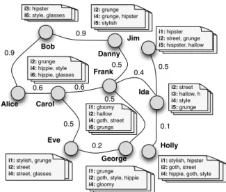
We believe that this simple model of triples for social data is the right abstraction for quite diverse types of social me-dia. Consider Tumblr [5]: one broadcasts posts to followers and rebroadcasts incoming posts; when doing so, the re-post is often tagged with chosen tags or short descriptions (hashtags). We can thus see a post and all its re-posted instances as representing one informational item, which may be tagged with various tags by the users broadcasting it. Text appearing in a blog post can also be in-terpreted as tags, provided either by the original author or by those who modified it during subsequent re-posts; it can also be exploited to uncover implicit tags, based on the co-occurrence of tags and keywords in text. Furthermore, a post that is clicked-on in response to a Tumblr search query can be seen as being effectively tagged (relevant) for that query’s terms. All this data has obviously a so-cial nature: e.g., besides existing follower/followee links, one can even use similarity-based links as social proximity indicators.EXAMPLE 1. We depict in Figure 1 a social network and the
tagging activity of its users, for a running example based on popu-lar tags from the fashion domain in Tumblr. There, for seeker Alice,
we have for instance, forα = 0.2, tf (glasses, i6) = 2,
sf (i6 | Alice, glasses) = σ(Alice, Bob) + σ(Alice, Carol)
= 0.9 + 0.6 = 1.5
f r(i6 | Alice, glasses) = 0.8 × 1.5 + 0.2 × 2
Extended proximity.
The model described so far takes into ac-count only the immediate neighbourhood of the seeker (the users iti3: hipster i6: style, glasses
i2: grunge i4: grunge, hipster i5: stylish
i2: grunge i4: hippie, style i6: hippie, glasses
i1: gloomy i2: hallow i4: goth, street i6: grunge
i1: hipster i2: street, grunge i5: hispster, hallow
i1: stylish, grunge i2: street
i4: street, glasses i1: grunge i2: goth, style, hippie i4: gloomy
i1: stylish, hipster i2: goth, street i4: hippie, goth, style
i2: street i3: hallow, h i4: style i5: grunge Alice Bob Carol Danny Eve Frank George Holly Ida Jim 0.9 0.6 0.5 0.6 0.9 0.5 0.5 0.5 0.2 0.1 0.4
Figure 1:Running example: social proximity & tagging. connects to explicitly). In order to broaden the scope of the query and go beyond one’s vicinity in the social network, we also account for users that are indirectly connected to the seeker, following a natural interpretation that user links and the query relevance they induce are (at least to some extent) transitive. To this end, we
de-note by σ+ the resulting measure of extended proximity, which is
to be computed from σ for any pair of users connected by at least
one path in the network. Now, σ+can replace σ in the definition
of social frequency Eq. (3).
For example, one natural way of obtaining extended proximity scores is by (i) multiplying the weights on a given path between the two users, and (ii) choosing the maximum value over all the
possible paths. Another possible definition for σ+ can rely on an
aggregation that penalizes long paths, in a controllable way, via an exponential decay factor, in the style of the Katz measures for social proximity [14]. More generally, any aggregation function that is monotonically non-increasing over a path, can be used here. Under this monotonicity assumption, one can browse the network of users on-the-fly (at query time) and “sequentially”, i.e., visiting them in the order of their proximity with the seeker.
Hereafter, when we talk about proximity, we refer to the ex-tended one, and, for a given seeker s, the proximity vector of s is the list of users with non-zero proximity with respect to it, or-dered decreasingly by proximity values (we stress that this vector is not necessarily known in advance).
EXAMPLE 2. For example, for seeker Alice, when extended
proximity between two users is defined as the maximal product of scores over paths linking them, the users ranked by
proxim-ity w.r.t. Alice are in orderBob : 0.9, Danny : 0.81, Carol :
0.6, F rank : 0.4, Eve : 0.3, George : 0.2, Ida : 0.16, J im : 0.07, Holly : 0.01.
The as-you-type search problem.
We consider in this pa-per a more useful level of search service for practical purposes, in which queries are being answered as they are typed. Instead of assuming that the query terms are given all at once, a more realistic assumption is that input queries are sequences of terms Q = [t1, . . . , tr], in which all terms but the last are to be matched exactly, whereas the last term tris to be interpreted as a tag poten-tially still in the writing, hence matched as a tag prefix.We extend the query model in order to deal with tag prefixes p by defining an item’s score for p as the maximal one over all possible
[4] ε [1] ε [2] ip [2] h [3] g [2] l [1] oomy [2] ster [2] pie [2] asses [2] oth [1] allow [4] st [3] y [2] lish [3] le [3] runge [4] reet (i4, 2) (i2, 1) (i6, 1) (i3, 1) (i2, 4) (i4, 2) (i2, 1) (i3, 1) (i5, 1) (i1, 2) (i3, 1) (i4, 1) (i5,1) (i1, 1) (i4, 1) (i6, 2) (i4, 1) (i2,2) (i4, 1) (i2, 3) (i1,2) (i4, 1) (i5,1) (i6,1) (i1, 2) (i5, 1) (i4, 3) (i2, 1) (i6, 1) IL(hipster) (i2, street, 4) (i4, style, 3) (i1, stylish, 2) (i5, stylish, 1) (i6, style, 1) virtual IL(st)
Figure 2:The CT-IL index.
completions of p:
sf (i | s, p) = max
t∈{p0s completions}sf (i | s, t) (5)
tf (p, i) = max
t∈{p0s completions}tf (t, i) (6)
(Note that when we compute the importance of an item, we might consider two different tag completions, for the social contribution and for the popularity one.)
EXAMPLE 3. If Alice’s query is hipster g, as g matches the
tags gloomy, glasses, goth and grunge, we have
sf (i4 | Alice, g) = max
t∈{g completions}sf (i4 | Alice, t)
= max[sf (i4 | Alice, gloomy),
sf (i4 | Alice, glasses), sf (i4 | Alice, grunge), sf (i4 | Alice, goth)]
= max[0.2, 0.3, 0.81, 0.41] = 0.81
4. AS-YOU-TYPE SEARCH ALGORITHMS
We revisit here the network-aware retrieval approach of [21, 25], which belongs to the family of early termination top-k al-gorithms known as threshold alal-gorithms, of which [8]’s TA (the Threshold Algorithm) and NRA (No Random-access Algorithm) are well-known examples.In the social-aware retrieval setting, when social proximity de-termines relevance, the data exploration must jointly consider the network (starting from the seeker and visiting users in descend-ing proximity order), the per-user/personal taggdescend-ing spaces, and all available socially-agnostic index structures such as inverted lists. It is thus important for efficiency to explore the social network by order of relevance/proximity to the seeker, as to access all the nec-essary index structures, in a sequential manner as much as possible. We favor such an approach here, instead of an incomplete “one di-mension at a time” one, which would first rely on one didi-mension to identify a set of candidate items, and then use the scores for the other dimension to re-rank or filter out some of the candidates.
4.1
Non-incremental algorithm
We first describe the TOPKS-ASYT approach for exclusively social relevance (α = 0) and without incremental computation, namely when the full sequence of terms is given in one keystroke, with the last term possibly a prefix, as Q = [t1, . . . , tr]. We fol-low an early-termination approach that is “user-at-a-time”: its main loop step visits a new user and the items that were tagged by her with query terms. Algorithm 1 gives the flow of TOPKS-ASYT.
Main inputs.
For each user u and tag t, we assume a precom-puted selection over the Tagged relation, giving the items tagged by u with t; we call these the personal spaces (in short, p-spaces). No particular order is assumed for the items appearing in a user list.We also assume that, for each tag t, we have an inverted list IL(t) giving the items i tagged by it, along with their term
fre-quencies tf (t, i)1, ordered descending by them. The lists can be
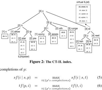
seen as unpersonalized indexes. A completion trie over the set of tags represents the access layer to these lists. As in Patricia tries, a node can represent more than one character, and the scores corre-sponding to the heads of the lists are used for ranked completion: each leaf has the score of the current entry in the corresponding inverted list, and each internal node has the maximal score over its children (see example below). This index structure is denoted hereafter the CT-IL index.
EXAMPLE4 (CT-ILINDEX). We give in Figure 2 an
illus-tration of the main components of CT-IL, for our running
exam-ple. Each of the tags has below it the inverted list (the one of the
hippietag is explicitly indicated). The cursor positions in the
lists are in bold. By storing the maximal score at each node (in brackets in Figure 2), the best (scoring) completions of a given pre-fix can be found by using a priority queue, which is initialized with the highest node matching that prefix. With each pop operation, ei-ther we get a completion of the prefix, or we advance towards one, and we insert in the queue the children of the popped node.
For comparison, we also illustrate in Figure 3 theCT-IL
in-dex that would allow us to process efficiently Alice’s top-k queries, without the need to resort to accesses in social network and p-spaces. Obviously, building such an index for each potential seeker would not be feasible.
While leaf nodes in the trie correspond to concrete inverted lists, we can also see each internal node of the trie and the corresponding keyword prefix as described by a “virtual inverted list”, i.e., the ranked union of all inverted lists below that node. As defined in Eq. (6), (5), for such a union, for an item appearing in entries of several of the unioned lists, we keep only the highest-scoring entry.
In particular, for the term tr of the query, by IL(tr) we refer to
the virtual inverted list corresponding to this tag prefix. There is one notable difference between the concrete inverted lists and the virtual ones: in the former, entries can be seen (and stored) as pairs (item, score) (the tag being implied); in the latter, entries must be the form (item, tag, score), since different tags (completions) may appear in such a list.
For each t ∈ {t1, . . . , tr}, we denote by top_item(t) the item present at the current (unconsumed) position of IL(t), we use top_tf (t) as short notation for the term frequency associated with this item, and, for IL(tr), we also denote by top_tag(tr) the tr completion in the current entry.
EXAMPLE5 (VIRTUAL LISTS). The virtual inverted list for
the prefix st is given in Fig. 2. Thetop_tag(st) is street, for
top_item(st) being i2, for its entry scored 4 dominates the one scored only2, hence with a top_tf (st) of 4. A similar one, for the
“personalized”CT-IL index for seeker Alice is given in Fig. 3.
Candidate buffers.
For each tag t ∈ {t1, . . . , tr−1}, we keepa list Dtof candidate items i, along with a sound score range: a
lower-bound and an upper-bound for sf (i | s, t) (to be explained hereafter). Similarly, in the case of tr, for each completion t of tr already encountered during the query execution in p-spaces (i.e., by triples (u, i, t) read in some u’s p-space), we record in a Dtlist
1
Even when α = 0, although social frequency does not depend directly on tf scores, we will exploit the inverted lists and the tf scores by which they are ordered, to better estimate score bounds.
[4] ε [1] ε [2] ip [2] h [3] g [2] l [1] oomy [2] ster [2] pie [2] asses [2] oth [1] allow [4] st [3] y [2] lish [3] le [3] runge [4] reet (i4,0.61) (i6,0.6) (i2,0.2) (i3,0.16) (i4,0.7) (i2,0.54) (i2,0.4) (i3,0.16) (i5,0.07) (i3,0.9) (i4,0.81) (i1,0.08) (i5,0.07) (i1,0.4) (i4,0.2) (i6,1.5) (i4,0.3) (i4,0.4) (i2,0.21) (i2,1.48) (i4,0.81) (i1,0.5) (i6,0.4) (i5,0.16) (i5,0.81) (i1,0.31) (i6,0.9) (i4,0.77) (i2,0.2) IL(hipster) (i6, style, 0.9) (i5, stylish, 0.81) (i4, style, 0.77) (i2, street, 0.54) (i1, stylish, 0.31) virtual IL(st)
Figure 3:Alice’s personalized CT-IL index.
the candidate items and their score ranges. Candidates in these D-buffers are sorted in descending order by their score lower-bounds. An item becomes candidate and is included in D-buffers only when it is first met in a T agged triple matching a query term.
For uniformity of treatment, a special item ∗ denotes all the yet unseen items, and it implicitly appears in each of the D-lists; note that, in a given Dtbuffer, ∗ represents both items which are not yet candidates, but also candidate items which may already be candi-dates but appear only in other D-buffers (for tags other than t).
Main algorithmic components.
When accessing the CT-IL index, inverted list entries are consumed in some IL(t) only when the items they refer to are candidates (they appear in at least one Dt0 buffer, which may not necessarily be Dtitself)2. We keep inlists called CILt(for consumed IL entries) the items read (hence
known candidates) in the inverted lists (virtual or concrete), for t being either in {t1, . . . , tr−1} or a completion of tr for which a triple (item, t, score) was read in the virtual list of tr. We also
record by the set C all tr completions encountered so far in
p-spaces. We stress that the trcompletions encountered in p-spaces
may not necessarily coincide with those encountered in IL(tr). For each t being either in {t1, . . . , tr−1} or a completion of tr already in C, by unseen_users(i, t) we denote the maximal num-ber of yet unvisited users who may have tagged item i with tag t. This number is initially set to the maximal possible term frequency of t over all items. unseen_users(i, t) then reflects at any mo-ment during the run of the algorithm the difference between the number of taggers of i with t already visited and one of either
• the value tf (t, i), if this term frequency has been read al-ready by accessing CT-IL, or otherwise
• the value top_tf (t), if t ∈ {t1, . . . , tr−1}, or • the value top_tf (tr), if t is instead a completion of tr. During the algorithm’s run, for known candidates i of some Dt, we accumulate in sf (i | s, t) the social score (initially set to 0).
Each time we visit a user u having a triple (u, i, t) in her p-space (Algorithm 2), we can
1. update sf (i | s, t) by adding σ+(s, u) to it, and
2. decrement unseen_users(i, t); when this value reaches 0, the social frequency value sf (i | s, t) is final.
The maximal proximity score of yet to be visited users is denoted max_proximity. With this proximity bound, a sound score range
for candidates i in Dtbuffers is computed and maintained as
• a score upper-bound (maximal score) MAXSCORE(i | s, t),
by max_proximity × unseen_users(i, t) + sf (i | s, t). 2
The rationale is that our algorithm does not make any “wild guesses”, avoiding reads that may prove to be irrelevant and thus leading to sub-optimal performance.
Algorithm 1 TOPKS-ASYT (non-incremental, for α = 0) Require: seeker s, query Q = (t1, . . . , tr)
1: for all users u do
2: σ+(s, u) = −∞
3: end for
4: for all tags t ∈ {t1, . . . , tr−1} do
5: sf (i | s, t) = 0
6: Dt= ∅, CILt= ∅
7: setIL(t) position on first entry
8: end for
9: setIL(tr) position on first entry
10: σ+(s, s) = 0;
11: C = ∅ (trcompletions)
12: H ← priority queue on users; init. {s}, computed on-the-fly
13: while H 6= ∅ do
14: u=EXTRACT_MAX(H); 15: PROCESS_P_SPACE(u); 16: PROCESS_CT-IL;
17: if termination condition then
18: break
19: end if
20: end while
21: return top-k items
• a score lower-bound (minimal score), MINSCORE(i | s, t),
by assuming that the current social frequency sf (i | s, t) is the final one (put otherwise, all remaining taggers u of i with t, which are yet to be encountered, have σ+(s, u) = 0). The interest of consuming the inverted list entries (Algorithm 3) in CT-IL, whenever top items become candidates, is to keep as accurate as possible the worst-case estimation on the number of unseen taggers. Indeed, when such a tuple (i, t, score) is accessed, we can do some adjustments on score estimates:
1. if i ∈ Dt, we can mark the number of unseen taggers of i with t as no longer an estimate but an exact value; from this point on, the number of unseen users will only change whenever new users who tagged i with t are visited, 2. by advancing to the next best item in IL(t), for t ∈
{t1, . . . , tr−1}, we can refine the unseen_users(i0 , t) es-timates for all candidate items i0for which the exact number of users who tagged them with t is yet unknown,
3. by advancing to the next best item in IL(tr), with some t = top_tag(tr) completion of tr, if t ∈ C, we can refine the
estimates unseen_users(i0, t) for all candidate items i0 ∈
Dt for which the exact number of users who tagged them
with t is yet unknown.
Termination condition.
From the per-tag Dtbuffers, we can infer lower-bounds on the global score w.r.t. Q for a candidate item (as defined in Eq. (2)) by summing up its score lower-boundsfrom Dt1, . . . , Dtr−1 and its maximal score lower-bound across
all Dt lists, for completions t of tr. Similarly, we can infer an
upper-bound on the global score w.r.t. Q by summing up score
upper-bounds from Dt1, . . . , Dtr−1and the maximal upper-bound
across all Dtlists, for completions t.
After sorting the candidate items (the wildcard item included) by their global score lower-bounds, TOPKS-ASYT can terminate whenever (i) the wildcard item is not among the top-k ones, and (ii) the score upper-bounds of items not among the top-k ones are less than the score lower-bound of the kth item in this ordering (we know that the top-k can no longer change).
As in [21], it can be shown that TOPKS-ASYT visits users who may be relevant for the query in decreasing proximity order and, importantly, that it visits as few users as possible (it is instance optimalfor this aspect, in the case of exclusively social relevance).
EXAMPLE 6. Revisiting our running example, let us assume
Algorithm 2 SUBROUTINE PROCESS_P_SPACE(u)
1: for all tags t ∈ {t1, . . . , tr−1}, triples T agged(u, i, t) do
2: if i 6∈ Dtthen 3: addi to Dt 4: sf (i | s, t) ← 0 5: unseen_users(i, t) ← top_tf (t) 6: end if 7: unseen_users(i, t) ← unseen_users(i, t) − 1 8: sf (i | s, t) ← sf (i | s, t) + σ+(s, u) 9: end for
10: for all tags t completions of tr, triplesT agged(u, i, t) do
11: if t 6∈ C then 12: addt to C, Dt= ∅ 13: end if 14: if i 6∈ Dtthen 15: addi to Dt 16: sf (i | s, t) ← 0 17: unseen_users(i, t) ← top_tf (t) 18: end if 19: unseen_users(i, t) ← unseen_users(i, t) − 1 20: sf (i | s, t) ← sf (i | s, t) + σ+(s, u) 21: end for
Algorithm 3 SUBROUTINE PROCESS_CT-IL
1: while ∃t ∈ Q s.t. i = top_item(t) ∈S
xDxdo
2: if t 6= trthen
3: tf (t, i) ← top_tf (t) (t’s frequency in i is now known)
4: advanceIL(t) one position
5: ∆ ← tf (t, i) − top_tf (t) (the top_tf drop)
6: addi to CILt
7: for all items i0∈ Dt\ CILtdo
8: unseen_users(i0, t) ← unseen_users(i0, t) − ∆
9: end for
10: end if
11: if t = trthen
12: t0← top_tag(tr) (some trcompletion t0)
13: tf (t0, i) ← top_tf (tr) (t0’s frequency in i known)
14: advanceIL(tr) one position
15: ∆ ← tf (t0, i) − top_tf (tr) (the top_tf drop)
16: addi to CILt0or setCILt0to {i} if previously empty
17: for all t00∈ C and items i0∈ D
t00\ CILt00do
18: unseen_users(i0, t00) ← unseen_users(i0, t00) − ∆
19: end for
20: end if
21: end while
(α = 0). The first data access steps of TOPKS-ASYT are as fol-lows: at the first execution of the main loop step, we visitBob, get
his p-space, addingi6 both to the Dstylebuffer and to aDglasses
one. There may be at most two other taggers ofi6 with style
(unseen_users(i6, style)), and at most one other tagger of i6 with glasses (unseen_users(i6, glasses)). No reading is
done inIL(style), as its current entry gives the non-candidate
itemi4, but we can advance with one pop in the virtual list of the
glprefix, for candidate itemi6. This clarifies that there is exactly
one other tagger with glasses fori6. After this read in the
vir-tual list of gl, we havetop_item(gl) = i1 (if we assume that
items are also ordered by their ids). At this pointmax_proximity
is0.81. Therefore, we have
MAXSCORE(i6 | Alice, style) = 0.81 × 2 + 0.9
MINSCORE(i6 | Alice, style) = 0.9
MAXSCORE(i6 | Alice, glasses) = 0.81 × 1 + 0.9
MINSCORE(i6 | Alice, glasses) = 0.9
We thus have thatscore(i6|Alice, Q) is between 1.8 and 4.23.
At the second execution of the main loop step, we visitDanny,
whose p-space does not contain relevant items forQ. A side-effect
of this step is thatmax_proximity becomes 0.6, affecting the
upper-bound scores above: score(i6 | Alice, Q) can now be
es-timated between1.8 and 3.6.
At the third execution of the main loop step, we visitCarol, and
find the relevant p-space entries fori4 (with tag style) and i6
(with tag glasses). Nowmax_proximity becomes 0.4. Also,
we can advance with one pop in the inverted list of style. This
clarifies that there areexactly 2 other taggers with style on i4,
and now we havetop_item(gl) = i1 and top_item(style) =
2. This makes score(i6 | Alice, Q) to be known precisely at 2.4, score(i4 | Alice, Q) to be estimated between 0.6 and 0.6 + 3 × 0.4 = 1.8, and score(∗ | Alice, Q) is at most 0.8.
4.2
Adaptations for the network-aware case
Due to lack of space, we only sketch in this section the neces-sary extensions to Algorithm 1 for arbitrary α values, hence for any textual-social relevance balance. When α ∈ [0, 1], at each iter-ation, the algorithm can alternate between two possible execution branches: the social branch (the one detailed in Algorithm 1) and a textual branch, which is a direct adaptation of NRA over the CT-IL structure, reading in parallel in all the query term lists (concrete or virtual). Now, items can become candidates even without being en-countered in p-spaces, when read in inverted lists during an execu-tion of the textual branch. As before, each read from CT-IL is asso-ciated with updates on score estimates such as unseen_users. For a given item i and tag t, the maximal possible f r-score can be ob-tained by adding to the previously seen maximal possible sf -score (weighted now by 1−α) the maximal possible value of tf (t, i); the latter may be known (if read in CT-IL), or estimated as top_tf (t) otherwise. Symmetrically, the minimal possible value for tf (t, i) is used for lower bounds; if not known, this can be estimated as the number of visited users who tagged i with t.
The choice between the two possible execution branches can rely on heuristics which estimate their utility w.r.t approaching the final result. Two such heuristics are explained in [21, 25], guiding this choice either by estimating the maximum potential score of each branch, or by choosing the branch that is the most likely to refine the score of the item outside the current top-k which has the highest estimated score (a choice that is likely to advance the run of the algorithm closer to termination).
4.3
Adaptations for incremental computation
We extended the approach described so far to perform the as-you-type computation incrementally, as follows:
1. when a new keyword is initiated (i.e., tr is one character
long), we take the following steps in order:
(a) purge all Dtbuffers for t ∈ C, except for Dtr−1(tr−1
is no longer a potential prefix, but a complete term), (b) reinitialize C to the empty set,
(c) purge all CILtbuffers for t 6∈ {t1, . . . , tr−1}, (d) reinitialize the network exploration (the queue H) to
start from the seeker, in order to visit again p-spaces looking for triples for the new prefix, tr. (This amounts to the following changes in Algorithm 1: among its ini-tialisation steps (1-12), the steps (4-8) are removed, and new steps for points (a) and (c) above are added.)
2. when the current tris augmented with one additional
char-acter (so tr is at least two characters long), we take the fol-lowing steps in order:
(a) purge Dtbuffers for t ∈ C s.t. t is not a trcompletion (b) remove from C all ts which aren’t completions for tr, (c) purge all CILtbuffers for t 6∈ {t1, . . . tr−1} ∪ C,
(d) resume the network exploration.
(This amounts to the following changes in Algorithm 1: among its initialisation steps (1-12), the steps (4-8) and (10-12) are removed, and new steps for points (a), (b), and (c) above are added.)
Note that, in the latter case, we can efficiently do the filtering op-erations by relying on a simple trie structure for directly accessing the data structures (D-lists, CIL-lists, the C subset) that remain valid for the new prefix.
4.4
Finding the most likely top-
kanytime
As argued before, we also see as crucial for the as-you-type search approach to have an anytime behaviour, in the following sense: it should explore the social space and existing data struc-tures / indexes in the most efficient manner, maintaining the candi-date buffers, until a time limit is met or an external event occurs. In-deed, in practice, we can expect that most searches will not meet the termination condition within the imposed time limit; when this hap-pens, we must output the most likely top-k result. In our case, this can be easily obtained from the intermediate result at any step in the TOPKS-ASYT computation, in particular the D-buffers, e.g., by adapting the more general SR-TA procedure (for Score-Ranges Threshold Algorithm) of [20], especially for the fact that we may have many D-buffers (if C is large). This calls for a different orga-nization, which is “per-item” instead of “per-tag”, for information in buffers Dtfor t ∈ C. In short, for each item i, we can keep in a trie structure the trcompletions t for which triples (user, i, t) have been encountered in p-spaces so far, with each leaf providing the score range for that item-tag pair. Further details are omitted here.
5.
EXPERIMENTS
We evaluate in this section the effectiveness, scalability and ef-ficiency of the TOPKS-ASYT algorithm. We used a Java imple-mentation of our algorithms, on a low-end Intel Core i7 Linux ma-chine with 16GB of RAM. We performed our experiments in an all-in-memory setting, for datasets of medium size (10-30 millions of tagging triples). We describe first the applications and datasets we used for evaluation.
5.1
Datasets
We used several popular social media platforms, namely Twitter, Tumblr, and Yelp, from which we built corresponding sets of (user, item, tag) triples. Table 1 reports some statistics about each dataset.
Twitter Tumblr Yelp
Number of unique users 458, 117 612, 425 29, 293
Number of unique items 1.6M 1.4M 18, 149
Number of unique tags 550, 157 2.3M 177, 286
Number of triples 13.9M 11.3M 30.3M
Avg number of tags per item 8.4 7.9 685.7
Avg tag length 13.1 13.0 6.5
Table 1: Statistics on the datasets we used in our experiments.
Twitter.
We used a collection of tweets extracted during Aug. 2012. As described in Section 3, we see each tweet and its re-tweet instances as one item, and the authors of the re-tweets/re-re-tweets as its taggers. We include both the text and the hashtags as tags.Tumblr.
We extracted a collection of Tumblr posts from Oct.-Nov. 2014, following the same interpretation on posts, taggers, and tags as in Twitter. Among the 6 different types of posts within Tum-blr, we selected only the default type, which can contain text plus images. Moreover, in the case of Tumblr, we were able to accessthe follower-followee network and thus we extracted the induced follower-followee network for the selected taggers.
Yelp.
Lastly, we considered a publicly available Yelp dataset, con-taining reviews for businesses and the induced follower-followee network.3 In this case, in order to build the triples, we considered the business (e.g., restaurant) as the item, the author of the review as the tagger, and the keywords appearing in the review as the tags. On Twitter and Tumblr datasets, in order to enrich the set of keywords associated to an item, we also expand each tag by the at most 5 most common keywords associated with it by a given user, i.e., by the tag-keyword co-occurrence. Finally, from the resulting sets of triples, we removed those corresponding to (i) items that were not tagged by at least two users, or (ii) users who did not tag at least two items.To complete the data setting for our algorithm, we then con-structed the user-to-user weighted networks that are exploited in the social-aware search. For this, we first used the underlying so-cial network (when available). Specifically, for each user pair in Tumblr or Yelp, we computed the Dice coefficient corresponding to the common neighbors in the social network. To also study sit-uation when such a network may not be available (as for Twitter), exploiting a thematic proximity instead of a social one, we built two other kinds of user similarity networks, based on the Dice co-efficient over either (i) the item-tag pairs of the two users, or (ii) the tags of the two users. We considered the filtering of “noise” links, weighted below a given threshold (as discussed in Section 5.2).
5.2
Experimental results: effectiveness
We present in this section the results we obtained in our exper-iments for effectiveness, or “prediction power”, with the purpose of validating the underlying as-you-type query model and the fea-sibility of our approach. In this framework, for all the data con-figurations we considered for effectiveness purposes, we imposed wall-clock time thresholds of 50ms per keystroke, which we see as appropriate for an interactive search experience.
To measure effectiveness, we followed an assumption used in recent literature, e.g. in [23, 21], namely that a user is likely to find his items – belonging to him or re-published by him – more interesting than random items from other users. For testing effec-tiveness, we randomly select triples (u,i,t) from each dataset. For each selected triple, we consider u as the seeker and t as the key-word issued by this user. The aim is to “get back” item i through search. The as-you-type scenario is simulated by considering that the user issues t one letter at a time. Note that an item may be re-trieved back only if at least one user connected to the seeker tagged it. We picked randomly 800 such triples (we denote this selection as the set D), for tags having at least three letters. For each indi-vidual measurement, we gave as input a triple (user, item, tag) to be tested (after removing it from the dataset), and then we observed the ranking of item when user issues a query that is a prefix of tag. Note that we tested effectiveness using single-word search for Twitter and Tumblr. On the contrary, for Yelp, due to its distinct features of having many triples per user, we did two-word search:
given a query q = (w1, w2), we first filtered items tagged by w1,
we then processed the remaining triples with query w2in the same
manner as we did for Twitter and Tumblr.
We define the precision P @k for our selected set D as
P @k =#{triple | ranking < k, triple ∈ D}
#D
Since this precision can be seen as a function of the main parame-ters of our system, our goal was to understand how it is influenced
3
1 2 3 4 5 6 7 8 l 0.0 0.1 0.2 0.3 0.4 0.5 0.6 0.7 0.8 P@5 Twitter item-tag α 0 0.01 0.1 0.4 1 1 2 3 4 5 6 7 8 l 0.0 0.1 0.2 0.3 0.4 0.5 0.6 0.7 P@5 Twitter tag α 0 0.01 0.1 0.4 1 1 2 3 4 5 6 7 8 l 0.0 0.1 0.2 0.3 0.4 0.5 0.6 0.7 0.8 0.9 P@5 Tumblr item-tag α 0 0.01 0.1 0.4 1 1 2 3 4 5 6 7 8 l 0.0 0.1 0.2 0.3 0.4 0.5 0.6 0.7 0.8 P@5 Tumblr tag α 0 0.01 0.1 0.4 1 1 2 3 4 5 6 7 8 l 0.0 0.1 0.2 0.3 0.4 0.5 0.6 P@5
Tumblr social network
α 0 0.01 0.1 0.4 1 1 2 3 4 5 6 7 8 l 0.00 0.05 0.10 0.15 0.20 0.25 P@5 Yelp item-tag α 0 0.01 0.1 0.4 1 1 2 3 4 5 6 7 8 l 0.00 0.05 0.10 0.15 0.20 0.25 P@5 Yelp tag α 0 0.01 0.1 0.4 1 1 2 3 4 5 6 7 8 l 0.00 0.05 0.10 0.15 0.20 0.25 0.30 0.35 0.40 P@5
Yelp social network
α 0 0.01 0.1 0.4 1
Figure 4:Impact of α on precision.
by these parameters. We describe below the different parameters we took into account here.
• l, length of the prefix in the query (number of characters). • θ, the threshold used to filter similarity links keeping only
those having a score above.
• α, the social bias (α = 0 for exclusively social score, α = 1 for exclusively textual score).
• ηi(u), the number of items tagged by user u, a user active-ness indicator (for simplicity, hereafter referred to as ηi). • ηu(i), number of users who tagged item i, an item popularity
indicator (ηu).
We present next the results we obtained for this experiment. (For space reasons, we only report here on P @5, but we performed test with P @1 and P @20 as well, which showcase similar evo-lution and improvement ratios, in the case of the latter, most often reaching precision levels of around 0.8-0.9.) When parameters are not variables of a figure, they take the following default values: α = 0 (fully social bias), θ is assigned the lowest value of the tested dataset, ηiand ηuare associated to active users and popular
items (ηi≥ 3 and ηu≥ 10).
1 2 3 4 5 6 7 8 l 0.1 0.2 0.3 0.4 0.5 P@5
Tumblr social network
θ 0.250 0.286 0.348 1 2 3 4 5 6 7 8 l 0.05 0.10 0.15 0.20 0.25 P@5 Yelp item-tag θ 0.050 0.060 0.078 1 2 3 4 5 6 7 8 l 0.00 0.05 0.10 0.15 0.20 0.25 P@5 Yelp tag θ 0.350 0.364 0.385 1 2 3 4 5 6 7 8 l 0.00 0.05 0.10 0.15 0.20 0.25 0.30 0.35 0.40 P@5
Yelp social network
θ
0.200 0.286 0.333
Figure 5:Impact of θ on precision.
Impact of
α.
As shown in Figure 4, α can have a major impact on precision. With a fully social bias (α = 0), we obtained the best results for the three datasets and all the available similarity networks. Moreover, typing new characters to complete the prefix increases the precision. However, the evolution for α = 0 can be quite slow, with the Tumblr or Yelp item-tag similarity network for witness. In this case, one likely reason is that these networks are quite rich in information, and the neighbors of the seeker are very likely to have the searched item, with the right tag, due to the way this network was built. This can also explain why the precision for the item-tag networks is higher in the case of Tumblr than those for tag and social similarity networks. The precision for the social similarity network is the lowest for Tumblr, while in the case of Yelp dataset the best results are obtained using the social network. Indeed, the tag and item-tag networks were built based on the same content we were testing on, whereas the social similarity network only uses the links between users to infer distances between them. Yelp exhibits lower precision levels overall, unsurprisingly, since it is a much denser dataset (number of triples per user).Interestingly and supporting our thesis for social bias, we obtain good precisions levels with such networks of similarity in social links (the highest in the case of Yelp). For example, in the case of Tumblr, we can reach P @5 of around 0.82 for the item-tag simi-larity network, 0.7 for the tag one, and still 0.5 for the social one. This indicates that we can indeed find relevant information using a content-agnostic network using TOPKS-ASYT. Importantly, it also indicates that we can always search with the same social sim-ilarity network, even when the content evolves rather rapidly, with the same precision guarantees.
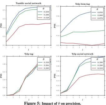
Impact of
θ.
In Figure 5, we can observe the impact of θ on the quality of results. We mention that the two highest θ values lead to 33% and 66% cuts on the total number of edges obtained with the lowest θ value. Unsurprisingly, removing connections between users decreases the precision. When using the similarity network filtered by the lowest θ value, the seeker is almost always connected to the network’s largest connected component, and we can visit many users to retrieve back the targeted item. With higher θ val-ues, the connectivity for certain seekers we tested with is broken, making some of the tested items unreachable.1 2 3 4 5 6 7 8 l 0.0 0.1 0.2 0.3 0.4 0.5 0.6 P@5
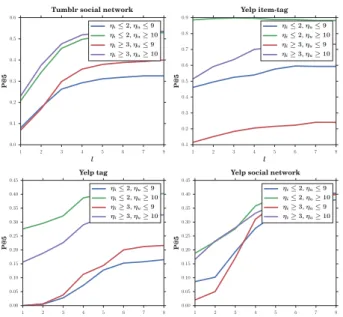
Tumblr social network
ηi≤ 2, ηu≤ 9 ηi≤ 2, ηu≥ 10 ηi≥ 3, ηu≤ 9 ηi≥ 3, ηu≥ 10 1 2 3 4 5 6 7 8 l 0.1 0.2 0.3 0.4 0.5 0.6 0.7 0.8 0.9 P@5 Yelp item-tag ηi≤ 2, ηu≤ 9 ηi≤ 2, ηu≥ 10 ηi≥ 3, ηu≤ 9 ηi≥ 3, ηu≥ 10 1 2 3 4 5 6 7 8 l 0.00 0.05 0.10 0.15 0.20 0.25 0.30 0.35 0.40 0.45 P@5 Yelp tag ηi≤ 2, ηu≤ 9 ηi≤ 2, ηu≥ 10 ηi≥ 3, ηu≤ 9 ηi≥ 3, ηu≥ 10 1 2 3 4 5 6 7 8 l 0.00 0.05 0.10 0.15 0.20 0.25 0.30 0.35 0.40 0.45 P@5
Yelp social network
ηi≤ 2, ηu≤ 9 ηi≤ 2, ηu≥ 10 ηi≥ 3, ηu≤ 9 ηi≥ 3, ηu≥ 10
Figure 6:Precision for various types of users and items.
Impact of popularity / activeness.
We show in Figure 6 the effects of item popularity and user activity for Yelp and Tumblr. For all similarity networks, the precision is better for popular items (high ηu). This is to be expected, as a popular item is more likely to be found when visiting the graph, as it is expected that it will score high since it has many taggers. Along with item popularity, we can observe that user activeness has a different effect in both content-based and the social similarity networks. Active users yield a better precision score when similarity comes from social links, whereas it is the opposite with content-based similarity networks. Reasonably, retrieving back an item for a non-active seeker in a content-based network is easier since his similarity with neighbours is stronger (Dice coefficient computed on less content).5.3 Experimental results: efficiency&scalability
In Figure 7, we display the evolution of NDCG@20 vs. time, for the densest dataset (Yelp), for different α values (where α is nor-malized to have similar social and textual scores in average). The NDCG is computed w.r.t. the exact top-k, that would be obtained running the algorithm on the entire similarity graph. This measure is an important indicator for the feasibility of social-aware as-you-type search, illustrating the accuracy levels reached under "typing latency”, even when the termination conditions are not met. In this plot, we fixed the prefix length size to l = 4. The left plot is when a user searches with a random tag (not necessarily used by her previ-ously), while the right plot follows the same selection methodology as in Section 5.2. Importantly, with α corresponding to an exclu-sively social or textual relevance, we reach the exact top-k faster than when combining these two contributions (α = 0.5). Note also that this trend holds even when the user searches with random tags. In Figure 8, similarly to the previous case, we show the evolution of NDCG@20 vs. time in Yelp, for different prefix lengths. (the left plot is for random tags). Results shows that with lower values of l we need more time to identify the right top-k. The reason is that shorter prefixes can have many potential (matching) items, therefore the item discrimination process evolves more slowly.In Figure 9 we show the evolution of NDCG@20 when visiting a fixed number number of users. We show results for l = 2, 4, 6. As expected, the more users we visit the higher NDCG we reach. For longer prefixes, it is necessary to visit more users. For instance, when l = 6, after visiting 500 users, we reach an NDCG of 0.8 while for l = 2 the NDCG after 500 visits is 0.9.
0 5 10 15 20 25 30 35 40 t(ms) 0.0 0.2 0.4 0.6 0.8 1.0 NDCG@20
Yelp social network
α 0.0 0.5 1.0 0 5 10 15 20 25 30 35 40 t(ms) 0.0 0.2 0.4 0.6 0.8 1.0 NDCG@20
Yelp social network
α 0.0 0.5 1.0
Figure 7:Impact of α on NDCG vs time for random search (left) and
personal search (right).
0 5 10 15 20 25 30 35 40 t(ms) 0.0 0.2 0.4 0.6 0.8 1.0 NDCG@20
Yelp social network
l 2 4 6 0 5 10 15 20 25 30 35 40 t(ms) 0.0 0.2 0.4 0.6 0.8 1.0 NDCG@20
Yelp social network
l 2 4 6
Figure 8:Impact of l on NDCG vs time for random search (left) and
personal search (right).
0 100 200 300 400 500
Number of visited users
0.0 0.2 0.4 0.6 0.8 1.0 NDCG@20
Yelp social network
l 2 4 6
0 100 200 300 400 500
Number of visited users
0.0 0.2 0.4 0.6 0.8 1.0 NDCG@20
Yelp social network
l 2 4 6
Figure 9:Impact of l on NDCG vs number of visited users for random
search (left) and personal search (right).
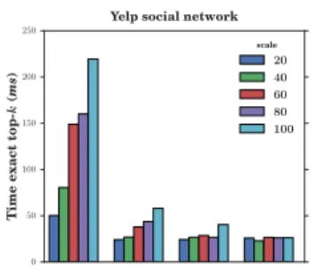
Finally, in the experiment illustrated in Figure 10 we observed the time to reach the exact top-k for different dataset sizes. For that, we partitioned the Yelp triples sorted by time into five consec-utive (20%) chunks. For each dataset we perform searches using prefixes of l = 2, 3, 4, 5. While the time to reach the exact top-k increases with bigger datasets and shorter prefixes, the algorithm scales adequately when l is more than 2. For instance, for l = 3, the time to reach the result over the complete dataset is just twice the time when considering only 20% of this dataset.
Main-memory vs. secondary memory considerations.
We emphasize here that we performed our experiments in an all-in-memory setting, for datasets of medium size (tens of millions of tagging triples), in which the advantages of our approach may not be entirely observed. In practice, in real, large-scale applications such as Tumblr, one can no longer assume a direct and cheap access to p-spaces and inverted lists, even though some data dimensions such as the user network and the top levels of CT-IL – e.g., the trie layer and possibly prefixes of the inverted lists – could still reside in main memory. In practice, with each visited user, the search might require a random access for her personal space, hence the interest for the sequential, user-at-a-time approach. Even when p-spaces may reside on disk, our last experiment shows that by retrieving a small number of them, less than 100, we can reach good precision levels; depending on disk latency, serving results in, for example, under 100ms seems within reach. One way to further alleviate such
2 3 4 5 l 0 50 100 150 200 250 T ime exact top-k (ms )
Yelp social network scale 20 40 60 80 100
Figure 10:Time to exact top-k for different dataset sizes. costs may be to cluster users having similar proximity vectors, and choose the layout of p-spaces on disk based on such clusters; this is an approach we intend to evaluate in the future, at larger scale.
6.
CONCLUSION
We study in this paper as-you-type top-k retrieval in social tag-ging applications, under a network-aware query model by which information produced by users who are closer to the seeker can be given more weight. We formalize this problem and we describe the TOPKS-ASYT algorithm to solve it, based on a novel trie data structure, CT-IL, allowing ranked access over inverted lists. In sev-eral application scenarios, we perform extensive experiments for efficiency, effectiveness, and scalability, validating our techniques and the underlying query model. As a measure of efficiency, since as-accurate-as-possible answers must be provided while the query is being typed, we investigate how precision evolves with time and, in particular, under what circumstances acceptable precision lev-els are met within reasonable as-you-type latency (e.g., less than 50ms). Also, as a measure of effectiveness, we analyse thoroughly the “prediction power” of the results produced by TOPKS-ASYT. We see many promising directions for improving the TOPKS-ASYT algorithm. First, for optimising query execution over the CT-IL index structure, we intend to study how CT-IL can be en-riched with certain pre-computed unions of inverted lists (materi-alised virtual lists). Assuming a fixed memory budget, this would be done for chosen nodes (prefixes) in the trie, in order to speed-up the sorted access time, leading to a memory-time tradeoff. While similar in spirit to the pre-computation of virtual lists of [18], a ma-jor difference for our setting is that we can rely on a materialization strategy guided by the social links and the tagging activity, instead of one guided by a known query workload. Also, one difficult case in our as-you-type scenario is the one in which tris the initial char-acter, following a number of already completed query terms. One possible direction for optimisation in TOPKS-ASYT is to avoid revisiting users, by recording the accessed p-spaces for future ref-erence. In short, within the memory budget, a naïve solution would be to keep these p-spaces as such (one per user). However, in or-der to speed-up the ranked retrieval, a more promising solution is to organise the p-spaces in a completion trie as well, which would allow us to access their entries by order of relevance.
Acknowledgements
This work was partially supported by the French research project ALICIA (ANR-13-CORD-0020) and by the EU research project LEADS (ICT-318809).
7.
[1] B. Bahmani and A. Goel. Partitioned multi-indexing: bringing orderREFERENCES
to social search. In WWW, 2012.
[2] H. Bast, C. W. Mortensen, and I. Weber. Output-sensitive autocompletion search. Inf. Retr., 11(4):269–286, 2008. [3] H. Bast and I. Weber. Type less, find more: Fast autocompletion
search with a succinct index. In SIGIR, 2006.
[4] F. Cai, S. Liang, and M. de Rijke. Time-sensitive personalized query auto-completion. In CIKM, 2014.
[5] Y. Chang, L. Tang, Y. Inagaki, and Y. Liu. What is Tumblr: A statistical overview and comparison. SIGKDD Expl., 16(1), 2014. [6] M. Curtiss, I. Becker, T. Bosman, S. Doroshenko, L. Grijincu,
T. Jackson, S. Kunnatur, S. Lassen, P. Pronin, S. Sankar, G. Shen, G. Woss, C. Yang, and N. Zhang. Unicorn: A system for searching the social graph. VLDB, 6(11), 2013.
[7] G. Das, D. Gunopulos, N. Koudas, and D. Tsirogiannis. Answering top-k queries using views. In VLDB, 2006.
[8] R. Fagin, A. Lotem, and M. Naor. Optimal aggregation algorithms for middleware. In PODS, 2001.
[9] J. Feng and G. Li. Efficient fuzzy type-ahead search in XML data. IEEE Trans. on Knowl. and Data Eng., 24(5), 2012.
[10] W. Hon, R. Shah, and J. S. Vitter. Space-efficient framework for top-k string retrieval problems. In FOCS, 2009.
[11] B.-J. P. Hsu and G. Ottaviano. Space-efficient data structures for top-k completion. In WWW, 2013.
[12] S. Ji, G. Li, C. Li, and J. Feng. Efficient interactive fuzzy keyword search. In WWW, 2009.
[13] D. Jiang, K. W.-T. Leung, J. Vosecky, and W. Ng. Personalized query suggestion with diversity awareness. In ICDE, pages 400–411, 2014. [14] L. Katz. Psychometrika, (1), Mar. 1953.
[15] P. Lagrée, B. Cautis, and H. Vahabi. A network-aware approach for searching as-you-type in social media - extended version. http://arxiv.org/abs/1507.08107/, 2015.
[16] G. Li, J. Feng, and C. Li. Supporting search-as-you-type using SQL in databases. IEEE Trans. on Knowl. and Data Eng., 25(2), 2013. [17] G. Li, S. Ji, C. Li, J. Wang, and J. Feng. Efficient fuzzy type-ahead
search in tastier. In In ICDE, pages 1105–1108, 2010.
[18] G. Li, J. Wang, C. Li, and J. Feng. Supporting efficient top-k queries in type-ahead search. In SIGIR, 2012.
[19] S. Maniu and B. Cautis. Taagle: Efficient, personalized search in collaborative tagging networks. In SIGMOD, 2012.
[20] S. Maniu and B. Cautis. Context-aware top-k processing using views. In CIKM, 2013.
[21] S. Maniu and B. Cautis. Network-aware search in social tagging applications: Instance optimality versus efficiency. In CIKM, 2013. [22] Q. Mei, D. Zhou, and K. Church. Query suggestion using hitting
time. In CIKM, 2008.
[23] M. Pennacchiotti, F. Silvestri, H. Vahabi, and R. Venturini. Making your interests follow you on twitter. In CIKM, 2012.
[24] M. Potamias, F. Bonchi, C. Castillo, and A. Gionis. Fast shortest path distance estimation in large networks. In CIKM, 2009.
[25] R. Schenkel, T. Crecelius, M. Kacimi, S. Michel, T. Neumann, J. X. Parreira, and G. Weikum. Efficient top-k querying over
social-tagging networks. In SIGIR, 2008.
[26] M. Shokouhi. Learning to personalize query auto-completion. In SIGIR, 2013.
[27] M. Shokouhi and K. Radinsky. Time-sensitive query auto-completion. In SIGIR, 2012.
[28] M. A. Soliman, I. F. Ilyas, and S. Ben-David. Supporting ranking queries on uncertain and incomplete data. VLDBJ, 19(4), 2010. [29] H. Vahabi, M. Ackerman, D. Loker, R. Baeza-Yates, and
A. Lopez-Ortiz. Orthogonal query recommendation. In RecSys, 2013. [30] S. Wu, J. Tang, and B. Gao. Instant social graph search. In
PAKDD12.
[31] S. Yahia, M. Benedikt, L. Lakshmanan, and J. Stoyanovich. Efficient network aware search in collaborative tagging sites. VLDB, 2008. [32] J. Zobel and A. Moffat. Inverted files for text search engines. ACM