Computational analysis of real-time convex optimization for control systems

(1)

Computational Analysis of Real-Time Convex

Optimization for Control Systems

by

Lawrence Kent McGovern

B.S., Aeronautics and Astronautics, M.I.T., 1994 M.S., Aeronautics and Astronautics, M.I.T., 1996

SUBMITTED TO THE DEPARTMENT OF AERONAUTICS AND ASTRONAUTICS

IN PARTIAL FULFILLMENT OF THE REQUIREMENTS FOR THE DEGREE OF

Doctor of Philosophy

at the

Massachusetts Institute of Technology

June, 2000

@

The author hereby grants to MIT pe ission to repro dice a to distribute copies of this thes' doc ent in whole o/in . of Authnr

Deyartment of Aei'onaus an Alstronautics ',Mav 4, 2000 Certified by

Eric Feron Associate Professor of Aeronautics and Astronautics

Thcis. Advisor

Certified by

/ 1 09 Brent Appleby

Charles Stark Draper Laboratory Committee Member

Certified by

Accepted by

Robert Freund Professor of Operations Research

A

n

Committee Member

James Paduano Principal Research Engineer, Dept. of Aeronautics and Astronautics

flrMmmitnt Mpmber

MASSACHUSETTS INSTITUTE _Chai OF TECHNOLOGY

SEP

0 7 2000

LIBRARIES

Nesbitt Hagood rman, Departmental Graduate Committee Signature

(2)

Computational Analysis of Real-Time Convex

Optimization for Control Systems

by

Lawrence Kent McGovern

Submitted to the Department of Aeronautics and Astronautics on May 4, 2000 in Partial Fulfillment of the

Requirements for the Degree of Doctor of Philosophy

Abstract

Computational analysis is fundamental for certification of all real-time control software. Nevertheless, analysis of on-line optimization for control has received little attention to date. On-line software must pass rigorous standards in reliability, requiring that any embedded optimization algorithm possess predictable behavior and bounded run-time guarantees.

This thesis examines the problem of certifying control systems which utilize real-time optimization. A general convex programming framework is used, to which primal-dual path-following algorithms are applied. The set of all optimization problem instances which may arise in an on-line procedure is characterized as a compact parametric set of convex programming problems. A method is given for checking the feasibility and well-posedness of this compact set of problems, providing certification that every problem instance has a solution and can be solved in finite time. The thesis then proposes several algorithm initialization methods, considering the fixed and time-varying constraint cases separately. Computational bounds are provided for both cases.

In the event that the computational requirements cannot be met, several alternatives to on-line optimization are suggested. Of course, these alternatives must provide feasi-ble solutions with minimal real-time computational overhead. Beyond this requirement, these methods approximate the optimal solution as well as possible. The methods ex-plored include robust table look-up, functional approximation of the solution set, and ellipsoidal approximation of the constraint set.

The final part of this thesis examines the coupled behavior of a receding horizon control scheme for constrained linear systems and real-time optimization. The driving requirement is to maintain closed-loop stability, feasibility and well-posedness of the op-timal control problem, and bounded iterations for the optimization algorithm. A detailed analysis provides sufficient conditions for meeting these requirements. A realistic exam-ple of a small autonomous air vehicle is furnished, showing how a receding horizon control law using real-time optimization can be certified.

Thesis Supervisor: Eric Feron

Title: Associate Professor of Aeronautics and Astronautics Technical Supervisor: Dr. Brent Appleby

(3)

(4)

Acknowledgments

I owe a great deal of thanks to many people who have contributed to the successful completion of this thesis. It has certainly been a long road, but also a fruitful and enjoyable one due to these people.

Professor Eric Feron undoubtedly deserves the greatest thanks for the guidance he has offered me over the years. He has always been more than generous with his time, even through his own busy schedule. Eric has a marvelous sense for unique problems worth pursuing, and always finds unconventional methods of attacking them. Also, his sense of humor has helped me to keep the right perspective, even if some of that French humor gets lost in translation.

I am indebted to Professor Robert Freund for his invaluable technical input. He has always offered outstanding advice, and many of his tips have turned into important cornerstones of this thesis. He is also one of the finest educators I have encountered during my decade at MIT, both in the lecture hall and in his office. I feel privileged to have benefited from his presence on my thesis committee, and also thank him for his long treks across campus from the operations research center to attend my meetings.

Dr. Brent Appleby has been my advisor and mentor at Draper Laboratory for six years now, and deserves much recognition. He has been a great resource through throughout my master's and doctoral work, providing both technical advice and helping me to manage the bureaucracy at Draper and MIT. I don't know how I could have navigated through graduate school without his help.

I also thank Professor James Paduano for his contributions as a member of my thesis committee. His critical questions have helped to make sure my thesis remained tied to reality and relevant to the field of aeronautics. Dr. Nicola Elia also deserves thanks for his input to my general examination, and for many interesting discussions in years past. Thanks go to Dr. Marc McConley and Dr. William Hall for joining my committee at the very end, and giving my thesis a good critical read. Marc waded through the text with a fine tooth comb, and uncovered many mistakes which I had completely overlooked. And Bill has been my one true resource on optimization at Draper Laboratory, as well as a good friend.

Special thanks to my friend and colleague Chris Dever, who did a nice job editing several chapters in this thesis. We have also enjoyed many lively discussions over food truck food, on bike rides, and at the Kendall Caf6, which have helped to distract me from the daily toil of student life.

Thanks to Nancy Masley from the graduate office (and from the radio station), for keeping an eye out for me. And a big thank you to the whole crew at WMBR, for an unforgettable five years. Am I ever going to miss that place!

(5)

A heartfelt thanks goes to Erika Garlitz, who has given me an immeasurable amount of support over the past year. She has been as good a friend as anyone could ever want. And she will be family in less than a month! I also want to thank my housemates, Joel Sindelar, Rich Diaz, and Nick Levitt, who have definitely improved the quality of my graduate student life.

My final thank you is reserved for my family. Mom & Dad, how could this ever have been possible without your love and support? And thanks too to my dear sister Wendy, and her fiance (and husband in just a few weeks) James Garlitz. Thank you all, who made this possible.

This thesis was prepared at The Charles Stark Draper Laboratory, Inc., under IR&D Project #15071. Publication of this thesis does not constitute approval by Draper of the findings or conclusions contained herein. It is published for the exchange and stimulation of ideas.

(6)

Nomenclature

R R+, R++ R7Q I R7++ Sn S"i, S~s+ E A -B A >-B (?, x) >Q 0 (7,x) >Q 0 I e ()T det(-) Det(-) A+ Amin(-), Amax(-) o-min() oma( Tr(-)

- set of real numbers

- set of real vectors of length n - set of real m x n matrices

= nonnegative and positive orthant

- the second-order cone (for n > 2)

the set of real symmetric n x n matrices

the set of positive semidefinite and positive definite n x n matrices

Hilbert space for conic program (see page 27)

A - B positive semidefinite, i.e., xT(A - B)x > 0 for all

x C 1R

A -B positive definite, i.e., xT (A -B)x > 0 for all x

c

Rn

= (y, x) E Rn+1 meaning _ > (En IX)1/2 = (Y, x) E Rn4, meaning - > (En 1 x) 1/2

identity matrix (dimension clear from context) vector of ones or 2.71828... (use clear from context)

= transpose

matrix determinant

= generalized determinant (see page 34) = Moore-Penrose inverse

= minimum and maximum eigenvalue of a matrix = minimum and maximum singular value of a matrix = trace of a matrix

(11)

log(.) H - 1 H 0 0 -HF 17(.) VB(-) V2_B(-) X,y,Z,... int X X, o, Z,... X o y

natural logarithm (base e)

= Euclidean vector norm, i.e.,

ia|l

=a Ta

= vector norm induced by H >- 0, i.e.,

|lx||H

V xTHx

vector infinity norm, i.e.,

|lail

₀ = maxi jail

Frobenius matrix norm, i.e.,

||AIIF

= TrATA

complexity order notation gradient of B(-)

Hessian of B(-)

= set

= interior of X

= element of Hilbert space E

(12)

Chapter 1 On-line Optimization in Feedback

Systems

The fields of optimization and control theory have long been interrelated. Quantitative performance criteria, such as the system 72 or 7.c norms, provide a measure of opti-mality for a control system. Coupled with the problem constraints, such as the system dynamics or modelling uncertainties, the control problem reveals itself as a constrained optimization problem. Over the last four decades, numerous controller synthesis tech-niques have emerged to solve these problems, a notable example being the linear quadratic Gaussian (LQG) optimal control problem [Mac89].

For some control problems, numerical optimization may be bypassed, and the best solution found analytically. This is the case for the LQG problem, in which a linear controller is derived from the solution to a set of algebraic Riccati equations. However, for slightly more general problems, an analytical solution is impossible, making numer-ical optimization a necessity. Histornumer-ically, these problems have not received as much attention because the computational requirements can be prohibitive. Over the years, some researchers have pointed out that numerical optimization problems with convex formulations are becoming tractable due to advancements in computational technology and convex programming algorithms. Early work on control design using numerical op-timization can be found in the publications of Fegley et al. [FBB+71], who used linear and quadratic programming. Subsequent work based on optimization of the Youla

(13)

rameterization has been done by Polak [PS89] and Boyd [BBB+88]. Linear programming has been the central tool of the recently developed f control theory [DDB94]. Finally, semidefinite programming has opened up a wide range of possibilities in system and control theory [BEFB94].

These recent control applications of mathematical programming can be seen as a direct offshoot of advances in computer technology. Problems which could not be realis-tically considered forty years ago are routinely solved today. The available computational resources will only continue to improve, so it makes sense to begin looking for the next step in taking advantage of these resources for control.

For most optimal control methodologies, including those mentioned above, the opti-mization phase is done entirely off-line. Because optiopti-mization tends to be fairly demand-ing computationally, on-line optimization has traditionally been viewed as impractical, especially for digital control systems which operate at relatively high frequencies. This aversion to on-line optimization has slowly been changing over the years, due to im-proved computational capabilities. Already, the chemical process industry has begun to embrace on-line optimization in the context of receding horizon control

[GPM89].

On-line methods allow the controller to directly incorporate hard system constraints such as actuator saturation, as well as treat future commanded inputs in an optimal manner. These methods also enable the controller to adapt to unforeseen changes that may take place in the system or constraints. The end product is a less conservative, more aggres-sive, and more flexible control system than could be designed off-line. The reason on-line optimization has been a practical tool for the chemical process industry is because the system dynamics of interest usually have fairly slow time constants, giving a computer the needed time to solve an optimal control problem in real time. In principle, given a fast enough computer, the techniques employed on these systems could be applied to a system of any speed.

In the near future, on-line optimization will become much more prevalent on faster systems. Of particular interest are aerospace systems, where high performance is desirable in the face of hard system constraints. The 1990s witnessed many potential uses for on-line optimization in the aerospace industry, from self-designing control systems for

(14)

15 high-performance aircraft to air traffic control. There is even a recent case where a linear programming algorithm was implemented on-line as part of an F-16 flight control system [MWBB97]. This example and several other proposed aerospace applications are discussed in Section 1.2.

While there is a wealth of literature on off-line optimization, the subject of on-line optimization is relatively unexplored. Very little research has been invested into deter-mining when it should be applied, how it should be applied, and the potential pitfalls. Philosophically, an on-line optimization algorithm is merely an information storage and retrieval mechanism, and therefore falls into the same category as look-up table or func-tion evaluafunc-tion. For any method of informafunc-tion retrieval, there is an inherent trade-off between accuracy of the information returned and the memory and computations re-quired to find that information. The decision to apply on-line optimization over some other method is dictated by the required accuracy and available processing power. For control systems, solution accuracy impacts closed-loop stability and performance. Linear feedback is efficient computationally, but may encounter loss in performance or stability when faced with system nonlinearities. Gain scheduling, a mixture of linear feedback and table look-up, is an improvement, yet carries a greater burden on memory, especially if the table dimension is large. Representing a control law using a mathematical pro-gram may offer the greatest amount of potential accuracy, but at much higher costs in computation. Understanding these computational costs is important to evaluating the appropriateness of an optimization algorithm for a particular application.

Computational analysis is fundamental for certification of on-line algorithms, yet to date has received little attention. There is a tendency among those who propose on-line optimization strategies to assume that the optimization problem can always be fully solved in the allotted time. However, this assumption cannot be taken on faith, since its violation can lead to disastrous consequences for the on-line procedure. To illustrate the importance of certification, consider the scenario where a linear program is embedded in a flight control system, and must be solved every second. Suppose next that at a particular time instance, the linear programming algorithm is presented with an ill-posed problem, and is not able to find a feasible solution within the allotted second. If this scenario has

(15)

not been anticipated, it could lead to failure of the flight control system, or worse yet, failure of the aircraft. Another conceivable scenario is that the optimization algorithm would return a feasible solution on schedule, but one which is far from optimality. In

Chapter 6 of this thesis, it will be seen that this, too, can lead to instability.

Certification means providing a guarantee that the optimization algorithm will deliver the desired solution by the appropriate deadline. By nature, optimization algorithms tend to vary in performance from problem to problem, and can be fairly unpredictable with few general guarantees. Even the best performing algorithms can run into unforeseen difficulties, and frequently an algorithm must be tuned to a particular problem. On the other hand, on-line software, especially flight code, must pass rigorous standards in reliability

[Lev95].

In particular, on-line software must have a deterministic run time. There is a general reluctance in industry to implement iterative algorithms on-line. If an upper bound on the number of iterations is known in advance, then a while loop can be replaced with a for loop, which is much more acceptable for on-line code. The most important trait an optimization algorithm must possess to meet this requirement is predictability. It is for this reason that conservative, predictable algorithms are preferred in this thesis over the more aggressive algorithms which tend to be used for off-line applications.

Determining the reliability of an on-line optimization procedure requires the ability to analyze sets of optimization problems, rather than unique problem instances. Of primary importance to this analysis is feasibility. Before implementation of an on-line procedure, the question must be asked: will every problem encountered be feasible? If the answer is no, then this indicates potential failure of the on-line method. Alternatively, it is impor-tant to determine whether there exist problem instances for which the objective function is unbounded, which can lead to an infinite computation time for an optimization algo-rithm. Once it is verified that every problem instance in a set is feasible, a computational upper bound must be determined. Depending on the processing power available to the application, this bound either can or cannot be met in the scheduled time. This is the

only way in which an optimization algorithm can be certified for an on-line application.

(16)

1.1. COMPLEXITY OF CONVEX PROGRAMMING

optimization using computational analysis. A careful computational analysis requires a clear understanding of how the optimization algorithm should be applied. This includes understanding how to initialize the algorithm intelligently, the theoretical worst-case convergence, and the accuracy at which the algorithm should terminate.

If stability and performance are taken as the driving requirements for the on-line

optimization procedure, then certification must consider the optimization algorithm and dynamic system as a whole. While initialization and convergence of the algorithm can be considered separately from the dynamic system, algorithm accuracy cannot, since the solution accuracy has a strong influence on the performance of the control system. At the very minimum, the controller should have enough accuracy to guarantee closed-loop

stability. Combining this requirement with a proper initialization of the algorithm and a

knowledge of the algorithm's rate of convergence, one can find the computational bounds necessary to certify an on-line optimization algorithm.

Understanding worst-case algorithm convergence requires a basic knowledge of com-plexity theory. The next section gives some background on algorithm comcom-plexity, which motivates the choice for the algorithms analyzed in this thesis.

1.1 Complexity of Convex Programming

The appropriate metric for comparison of an algorithm's worst-case performance comes

from complexity theory. An upper bound on the complexity of an algorithm is indicated

using the order notation 0(-). Given two sequences of scalars {N,} and {S}, the notation

Nn = 0(Sn)

indicates that

Nn < C Sn

for some positive constant C and for all n sufficiently large. In the case of optimization algorithms, N, usually refers to the number of computations or iterations required of the 17

(17)

algorithm for a problem of dimension n, and So, is some function of n. Complexity the-ory generally distinguishes between two types of algorithms, polynomial and exponential. An algorithm is considered polynomial if S, is a polynomial of n (e.g., nP) and exponen-tial if S, is an exponenexponen-tial function (e.g., p"). Since exponenexponen-tial functions grow at an enormously fast rate, exponential algorithms are intractable on the worst-case problem except when the dimension is very small.

Worst-case analysis is an important tool for certification. Since on-line algorithms must at least be tractable on the worst-case problem instance, only polynomial time algorithms are considered in this thesis. For the most part, this restricts the types of problems which may be considered to convex programs, although there are a few nonconvex problems which can be solved in polynomial time (e.g., many problems in network optimization have this property).

Complexity considerations also restrict the attention of this thesis to interior-point methods. The seminal work of Nesterov and Nemirovskii

[NN94]

has given polynomial complexity results for interior-point methods in a general convex programming frame-work. In practice, interior-point methods are also competitive with other optimization methods, and have been observed to outperform other commonly used methods (e.g., the active set method) as the problem dimension increases [GB98]. Due to this practical value, interior-point methods have been proposed for receding horizon control by several authors [GB98, HanOO, RWR98].

Currently, there is no known algorithm for which the complexity of finding an exact solution to a convex program is polynomial in the problem dimension, even in the case of linear programming. Many complexity results for linear programming show a dependence on the bit-size of the problem. Alternatively, Renegar [Ren95a] has shown that the complexity can also be related to the condition number of the linear program (condition numbers for convex programs are analogous to matrix condition numbers, discussed more in Chapter 3).

Rather than determining the complexity of finding an exact solution to a convex programming problem, it is reasonable to consider the complexity of finding a solution which is within a tolerance e of optimality. Through the use of interior-point algorithms,

(18)

1.1. COMPLEXITY OF CONVEX PROGRAMMING

an c-optimal solution can be determined with polynomial complexity in the problem dimension and conditioning.

Interestingly, the most celebrated convex optimization algorithm, the simplex method for linear programming, is an exponential algorithm. This was noted by Klee and Minty

[KM72], who discovered a now famous example requiring 2" iterations to solve a linear program in R. This is in spite of the fact that the simplex algorithm performs exception-ally well on most problems. Similarly, other boundary-traversing convex programming algorithms such as active set methods for quadratic programming also have exponential

complexity in spite of good practical performance [Fle87]. The first polynomial-time algorithm was the ellipsoid algorithm, discovered in 1979 by Khachiyan [Kha79].

Unfor-tunately, this algorithm performs on average as slow as its theoretical worst case, and is not competitive with the simplex method on even the smallest problems.

Karmarkar was the first to propose a practical polynomial-time algorithm for linear programming [Kar84], which has an O(nlog(1/c)) iteration bound. Karmarkar's method is the precursor to most current interior-point algorithms, the best of which have an O(Vnlog(1/E)) complexity. The main distinction between Karmarkar's method and modern interior-point algorithms is that most of today's algorithms consider the primal and dual problems simultaneously, whereas Karmarkar's method is primal-only. It is to

this primal-dual formulation that the best interior-point methods owe their efficiency.

Since worst-case performance has great relevance to real-time optimization, the

inter-ior-point algorithms used in this thesis are those with the best known complexity bound O(Fnlog(1/E)), rather than the algorithms that tend to perform best in practice. The

O(j"log(1/c)) algorithms tend to take short, conservative steps towards the optimal

solution, and employ very few heuristics. Ironically, many of the algorithms which tend to perform better by taking much more aggressive steps towards the optimal solution actually have larger complexity values (e.g., the long-step algorithm is O(n log(1/E))), and some of the best performing algorithms have no guarantees whatsoever. It is the contention of this thesis that these "more aggressive" interior-point methods are less suitable for on-line optimization, not only because of their larger complexity bounds, but also because they may be less predictable due to their heuristics.

(19)

1.1.1 Linear Convergence and Iteration Bounds

The algorithms discussed in the next chapter belong to a class known as path-following algorithms. Bounds in the number of iterations follow by proving a certain rate of linear convergence towards the optimal solution. The algorithms examined here are primal-dual, meaning the degree of optimality is measured by the duality gap p > 0, where p = 0 indicates primal-dual optimality. The best known convergence bounds satisfy

I'1k+1 < - ) Yk

where Pk is the duality gap at iteration k, A > 0 is a constant, and n is the problem dimension. Given this linear convergence rate, an objective Pk CPo is satisfied for all

k > K =' lge - | [log(1 -zA/V) ) Noting that log(1 + )

0,

it follows that

K < [\ log(1/) therefore, K = O(Vlog(1/c)).

Despite the fact that the predicted number of iterations is polynomial, it can still be very large when compared to actual algorithm performance. This is because the value of (1 - A/") can be very close to 1. In reality, the ratio yk+1/pk is frequently much smaller than its theoretical bound. For some of the more aggressive algorithms, the ratio is often about 0.1. Convergence of the path-following algorithms used in this thesis is not quite that good, but still tends to be better than its theoretical worst case. It may be possible that smaller guaranteed ratios for pk+1/pk can be proved for particular problem instances, which would result in much more realistic iteration bounds.

1.2 Applications of On-Line Optimization

The potential applications of on-line optimization are virtually limitless. A few moti-vating examples are given in this section to show the importance of on-line optimization for control systems. These examples are real engineering control methodologies which

(20)

1.2. APPLICATIONS OF ON-LINE OPTIMIZATION

require on-line optimization, and the success of these methods depends on the delivery of the solution to a convex program at regularly scheduled time intervals.

1.2.1 Receding Horizon Control

At present, receding horizon control is the most widely used on-line optimization control method in industry. It has been the accepted standard for constrained multivariable problems by the chemical process industry for over two decades. Its strength is an abil-ity to directly incorporate state and input constraints into the design, as well as future command inputs. In its most typical form, receding horizon control is solved as a linear or quadratic program, although recent developments in convex programming have al-lowed researchers to consider more sophisticated formulations. For example, control laws which are robust to modeling uncertainty are presented in [KBM96] using semidefinite programming and in [BCH98] using second-order cone programming. A more standard formulation is given below.

Given a linear time invariant system, a typical problem in receding horizon control is posed as the open-loop optimal control problem

N-1

min ((Yk - rk)' y - rk) + uiRuk) + XNPXN

k=O

subject to Xk+1 = Axk + Buk

Yk CXk + Duk

Ymin Yk Imax

Umin Uk < Umax

where rk is a target trajectory for output Yk, and P, Q, and R are weighting matrices. This problem is solved on-line as a quadratic program. Only the first control input uo is implemented, and the problem is resolved at the next time step.

The drawback to receding horizon control is the relatively high computational effort when compared to linear feedback control laws. This has traditionally limited the use of receding horizon control to the slow dynamic systems typically encountered in the chemical process industry. However, the range of applications is beginning to expand as greater computing power becomes available. In Chapter 6, the subject of receding

(21)

horizon control is explored in greater depth, and applied to a higher bandwidth aerospace example.

1.2.2 Control Allocation

As aircraft become increasingly sophisticated, the number of moment generating actua-tors increases far beyond the conventional number of three independent actuaactua-tors. For example, the F-18 HARV (High Angle-of-attack Research Vehicle) has rudders, horizon-tal tails, ailerons, leading edge and trailing edge flaps (each left and right), as well as three thrust vectoring moment generators, for a total of 13 independent moment inputs.

Current proposals for tailless aircraft show the possibility of up to 20 independent actu-ators. These systems are clearly overactuated, yet are subject to saturation constraints on the control surfaces. The control allocation problem is motivated by the desire to choose the optimal configuration of the actuators to meet a specified objective, subject to saturation constraints. Furthermore, it allows the possibility of mitigating actuator failure. An introduction to the control allocation problem is found in [Dur94, Enn98). An application of control allocation to a tailless fighter aircraft is given in [Buf97].

The standard form for the control allocation problem follows below. The linear equa-tion d = Bu maps the control input u E R' to a moment d C R' via the matrix B,

derived from the linearized dynamics of the aircraft. A set of constraints umi < u 5 Umax defines the saturation constraints of the actuators. The objective is to achieve a desired moment ddes. If ddes is not feasible, a weighted 2-norm of the error may be minimized instead, i.e., mineTWe where e = ddes - Bu and W is a symmetric, positive definite

matrix. Alternatively if ddes is feasible, then a weighted distance from u to a preferred control up may be minimized, i.e., min(u - up)TW(u - up).

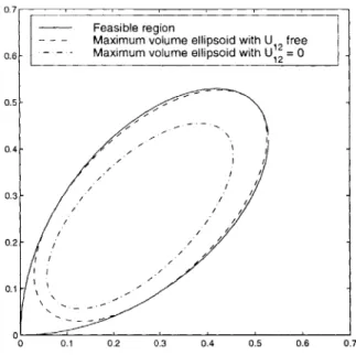
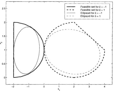
As presented, the control allocation problem is an on-line quadratic program. How-ever, control allocation is generally not implemented as a quadratic program due to the inherent difficulty in certification of on-line optimization. A number of alternatives are given in [Enn98]. One recently proposed strategy is to approximate the feasible space by an ellipsoid [OJMF99]. Chapter 5 explores alternatives to on-line optimization similar to this.

(22)

1.2. APPLICATIONS OF ON-LINE OPTIMIZATION

1.2.3 Reconfigurable Control

Over time, the closed-loop dynamics of a system are capable of changing in unexpected ways. Changes may happen either gradually or immediately, as in the case of actuator failure. The term "reconfigurable control" simply refers to any control system capable of redesigning itself to meet a new set of dynamics. It usually involves some form of on-line system identification, coupled with a control redesign procedure. Reconfigurable control has been of particular interest to high-performance fighter aircraft, for which an unanticipated change in the open-loop dynamics can have disastrous consequences. In

[PCM95],

a basic reconfigurable control strategy is proposed for aerospace applications. In 1996, a reconfigurable control law was successfully flight tested on the VISTA/F-16 by Barron Associates, Inc. [MWBB97]. Part of this flight test included a landing of the aircraft in crosswind conditions with a simulated missing left horizontal tail. The control system included a parameter identification algorithm which identified the stability and control derivatives on-line, in concert with a receding horizon control algorithm based on linear programming. Since then, similar strategies have been suggested for tailless aircraft as part of the Reconfigurable Systems for Tailless Fighter Aircraft (RESTORE) program at Lockheed Martin [EW99] and for Vertical Take-Off/Landing (VTOL) Uninhabited Air Vehicle (UAV) automated shipboard landing [WMS99].

1.2.4 Combinatorial Applications

It might seem limiting that this thesis only considers convex optimization, since many interesting on-line applications are nonconvex in nature. Combinatorial problems are abundant in the real world, most of which fall into the class of NP-hard problems (a class of problems which do not appear to be solvable in polynomial time). The usual approach to attacking these problems is using heuristics, which carry little if any guaran-tees. Fortunately, many of these problems have convenient convex relaxations, and thus can be attacked using convex programming. Convex relaxations can be derived using Lagrangian duality, since the dual of the dual is always convex. Combinatorial problems involving constraints such as x E {0, 1} are frequently replaced with quadratic

(23)

straints x2 - x = 0, which have semidefinite programming relaxations [L099]. Many

combinatorial and quadratic problems with good semidefinite relaxations have been noted in the literature, including MAX-CUT, graph coloring, and quadratic maximiza-tion [GW95, KMS98, Zha98, Ali95]. There are diverse real-world applicamaximiza-tions of these problems, from circuit design to cellular phone channel assignment.

One relevant aerospace application is aircraft conflict detection and resolution. As the skies become increasingly congested with aircraft, air traffic controllers face the dif-ficult task of rerouting traffic such that aircraft remain separated by a minimum dis-tance. Given a set of aircraft positions and trajectories, one would ideally like to find the minimum change in trajectory necessary for a conflict-free path. This problem is combinatorial because, for example, each aircraft must decide whether to steer to the left or right of each other aircraft. In [FMOFOO], this problem is posed as a nonconvex quadratically-constrained quadratic program, and the convex relaxation is proposed as an on-line optimization technique.

1.3 Thesis Objectives and Organization

The ultimate goal of this thesis is to show that optimization can be certified for on-line applications. Certification is necessary for any software which must run in real time, but becomes especially important for aerospace applications, where software failure can mean loss of the vehicle and/or loss of life. For this reason, the emphasis of this thesis is about what can be proved about an on-line algorithm, rather than what can be inferred from simulation. The guarantees given in this thesis are conservative by nature, and reflect the current gap between theory and practice which exists in the field of optimization.

Chapter 2 introduces much of the relevant background material on convex optimiza-tion. Convex optimization is presented in a fairly general form, as conic convex pro-gramming over the class of symmetric cones. This allows the contents of this thesis to be applied to linear programming, second-order cone programming (to which convex quadratic programming belongs), and semidefinite programming. Chapter 2 focuses on one class of interior-point algorithms: primdual path-following algorithms. These

(24)

al-1.3. THESIS OBJECTIVES AND ORGANIZATION

gorithms are used because they have a very predictable behavior, and they have the best known complexity bounds. These two qualities are of high importance to safety-critical on-line systems. Finally, homogeneous self-dual programming is described, which is very reliable and easy to initialize. Homogeneous self-dual programming will become useful in subsequent chapters.

On-line optimization problems are typically parameter dependent problems, in which the parameter changes from instance to instance, but always belongs to some bounded set. Chapter 3 takes the important step of placing convex programming in a parameter dependent framework. These problems are parameterized using linear fractional transfor-mations, which are seen as fairly general means of representing rational functions. Using this parameterization, solutions which are robustly feasible to parameter variations are introduced. Background material is given for the convex programming condition number, which gives a normalized measure of the proximity of a problem to infeasibility. Both condition numbers and robustly feasible solutions are used in later sections. In the last part of this chapter, a methodology is presented for checking whether every problem in a parametric space is feasible. This technique uses a branch-and-bound technique, although it is seen that checking feasibility can be made considerably easier if the parameterization has a certain form.

The heart of the thesis is Chapter 4, where computational bounds are given for parameter-dependent convex programming. In the first part, the constraints are consid-ered to be fixed, and only the objective function is free to vary. An initialization strategy is proposed for this problem, and corresponding computational bounds derived. The sec-ond part explores the case where both constraints and objective are time-varying. Both the big-M method (a well-known, basic infeasible start method) and homogeneous self-dual programming are explored for initialization. The analysis focuses on homogeneous self-dual programming, since it tends to be the more efficient means of initialization. A branch-and-bound technique is used for deriving computational bounds.

On-line optimization can be computationally demanding. On top of that, the compu-tational bounds derived in Chapter 4 tend to be conservative. For the instances when the computational demands of on-line optimization become too great, it is desirable to find

(25)

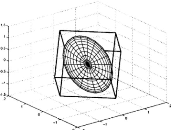
cheap alternatives. Chapter 5 explores several options for approximating the solution to a parametric convex program. A few of the obvious choices of solution approximation are explored, such as look-up tables and function approximation. A fair portion of this chapter is devoted to approximating a set of constraints with an ellipsoid. Because of the relative ease of optimizing a linear objective over an ellipsoid, this approximation strategy is very simple to implement as part of an on-line algorithm.

Chapter 6 is devoted to the most common control application of on-line optimization: receding horizon control. The most essential certification requirement of any on-line con-trol algorithm is stability. For receding horizon concon-trol, the necessary theory is developed to show that on-line optimization can stabilize constrained linear systems. This result goes beyond the traditional assumption for receding horizon control: that an on-line optimization algorithm exists which delivers an optimal solution at the scheduled time. This stability requirement drives the minimum accuracy which must be requested of the optimization algorithm, ultimately resulting in a computational bound for the algorithm.

The final part of Chapter 6 demonstrates real-time optimization on a realistic control example. A receding horizon control approach is proposed for an uninhabited air vehicle (UAV) example, where the actuator saturation is significant enough to induce closed-loop instability. Computational bounds are derived for the on-line scheme, providing a means of certifying this control approach.

A summary of the technical contributions of this thesis is found in Chapter 7, but there is one contribution which is more philosophical that needs to be emphasized. There is currently a gap between the optimization and control communities which frequently goes unnoticed. Control engineers tend to avoid applying on-line optimization strategies out of a mistrust of iterative algorithms, which are seen as unpredictable. Operations researchers often approach optimization from an off-line perspective, devising heuristics which seem to improve performance of the algorithms, yet do not address the concerns of on-line optimization. Complexity theory has opened the door to certification of these algorithms for on-line use. The better this message is understood, the more likely on-line optimization will be trusted and used in future applications.

(26)

Chapter 2 Convex Programming

The term convex programming refers to any optimization problem minzxE f(x) in which the objective f (x) is a convex function and the constraint set X is a convex set. Convexity is of great importance to optimization for many reasons, the most important being that any local optimum is immediately known to be globally optimal. In Chapter 1, it was stated that from a complexity point of view, the most efficient known algorithms for convex programming are primal-dual interior-point algorithms. This chapter provides the details on a few interior-point algorithms, and also presents some of the supporting theory needed for development of these algorithms.

2.1 Conic Convex Programming

This thesis is concerned primarily with the conic convex optimization problem

inf cT x

subject to X = To + Fx (2.1)

I E E,7

where c, X E R", X and To belong to some finite-dimensional Hilbert space E , F is a linear operator from R" to E, and K C E is a convex cone. Later on, KC will be restricted to the class of symmetric cones, defined in Section 2.3, but at the moment this restriction is not needed. In convex programming, the space E is generally a space of real or complex

(27)

vectors or matrices.

The conic form given by (2.1) is very general. In fact, Nesterov and Nemirovskii [NN94] point out that any convex programming problem can be written in this form. Sev-eral important types of convex programming problems are linear programming, second-order cone programming and semidefinite programming, which are introduced below.

Linear Programming The linear program is perhaps the most well-understood convex programming problem, often written as

min cTx x

subject to Ax < b

The convex cone IC is simply the non-negative orthant Rn+. The most famous algorithm for solving a linear program is the simplex method, which produces iterates that travel along the vertices of the polyhedron defined by Ax < b. While the simplex method tends to work well in practice, its exponential worst-case complexity has led researchers to consider alternative polynomial-time interior-point methods.

Second-Order Cone Programming The second-order cone, also known as the

Lor-entz cone or "ice-cream" cone, is described by the set

t=

{(

x) E RxIR 7I >

||

x||}.

The notation [y x]T >Q 0 is used to indicate (-y, x) c R'gt. Linear programming, convex quadratic programming, and quadratically constrained quadratic programming are all special cases of second-order cone programming. An excellent overview of many other problems which may be formulated as a second-order cone program is found in [LVBL98].

Semidefinite Programming Semidefinite programming is simply the minimization of a linear objective subject to a linear matrix inequality, described by

inf cTx

subject to Fo + Fixi >- 0,

i=1

where F0, ... ,Fm E S". The notation A >- 0 indicates that a symmetric matrix A is

positive semidefinite. The cone of all semidefinite matrices of dimension n is indicated by S".

(28)

2.1. CONIC CONVEX PROGRAMMING 29 Sometimes it will be convenient to use the vector-space notation

'To = svec(FO), (2.2)

F _{svec(F) -.} _svec(Fm)j,

where svec(.) maps the subspace of symmetric matrices in S' to Rn(n+1)/2 _{with the}

convention

svec(A) = [all, Va12, . .. , 2dain, a22, . .. , da2n, . ann ,

and aj is the ij entry of A. This convention ensures that the inner product (A, B) A TrAB satisfies

(A, B) = svecATsvecB = (svec(A), svec(B)).

The notation smat(-) indicates the inverse of svec(.). The vectorization of the positive

semidefinite cone S" is written as VS"+, i.e., V E VS" <- smat(v) E S"+

Semidefinite programming is the most general of the three convex programs considered here, since the linear constraint Ax < b can be written as diag(b - Ax) S 0, and the second-order cone constraint

||xfl

< -y as

[rI x]

X _0.

However, from a complexity point of view it is better to consider a semidefinite constraint using linear or second-order conic constraints whenever possible. To find a solution which is E from optimality, the best known interior-point algorithms for semidefinite programming take 0(1n log(1/c)) iterations, with 0(n4_{) computations per iteration for}

a dense matrix. A linear program has the same iteration complexity, with only 0(n 3₎

computations per iteration. This difference in per-iteration complexity is due to the block-diagonal structure of the linear program when posed as a semidefinite program.

The benefit of using a second-order cone is much more dramatic. To see this impact, consider the problem

min y

subject to ;>Q 0

(29)

where A E R"Xm and b EE R. If this problem is solved using a second-order cone pro-gramming interior-point method, it can be solved to e accuracy in 0(log(1/E)) iterations,

regardless of the dimensions m and n [LVBL98]. This is compared to the "equivalent"

semidefinite program min -y subject to Ax+b XTA + bT 0 10

which is solved in O(vm + 1 log(1/e)) iterations. In addition, the amount of work per iteration of the second order cone program is 0(n'), compared to 0(n 4) for the

semidef-inite program. From this assessment, the second-order cone format is preferable to the more general semidefinite programming format.

2.2 Duality

Associated with any convex conic program the dual:

is another convex conic program known as

sup - (To, Z) z

subject to F TZ = c

Z E K*, where KC* is the dual cone of K, defined as

K* = {Z I (X Z) > 0, VX E K}. Letting E = RN, observe that the dual problem

writing

inf yERN subject to

can be put in "primal" form (2.1) by

bT y + d

Z= 90 +Gy

Z E IC*,

(30)

2.2. DUALITY where 9_o₌_(F+)Tc G I - (F+)TF T b=GT'To d =(70,7 9o),

and F+ indicates the Moore-Penrose inverse of F, e.g., F+ = (FTF)-FT when F has full column rank. Since G is a rank N - r matrix, where r is the rank of F, the dimension of

y can be reduced to N - r, and the dimension of G reduced from N x N to N x (N - r).

Let p* denote the optimal value of the primal, and d* the optimal value of the dual, i.e.,

p inf{cTx I To + Fx E K}

x

d* A sup{--(To, Z) FTZ = c, Z E K*}.

z

In general, inf and sup cannot be replaced by min and max, since the optimal values may not be achieved.

The duality gap between primal and dual feasible variables is defined as the difference

between primal and dual objective values, and is seen to be non-negative by the relation

XTC + (To, Z) = (x, FT_{Z) + (To, Z) = (I, Z) > 0.}

From this, it is clear that weak duality holds for any conic problem, meaning p* > d*.

A stronger duality result is possible given certain constraint qualifications. These qualifications are based on the feasibility of the primal and dual problems, so a few definitions are required. Let the primal and dual feasible sets be defined by

Fp {XIX X= To + F E C, x E R"} FD {ZI FTZ c, Z E K*},

and the interiors defined by

0

TP Fp n int K

.FD FDn int .

(31)

Definition. A primal or dual problem is said to be feasible if _F 5 0, otherwise it is

infeasible. A feasible problem is strongly feasible if .:L 0. Otherwise it is weakly

feasible.

Strong feasibility is sometimes known as the Slater condition, and ensures strong duality, defined in the next theorem.

Theorem 2.1. If the primal or dual problem is strongly feasible then strong duality

holds, meaning p* = d*. Furthermore, if both the primal and dual are strongly feasible,

then the optimal values p* and d* are achieved by the primal and dual problems, i.e., inf and sup can be replaced by min and max.

This theorem is a well-known result of convex programming, see for instance Rock-afellar

[Roc70),

also Luo et al. [LSZ97] for many other duality results. The zero duality gap of a strongly dual problem is also known as the complementary slackness condition, where optimizers X* and Z* satisfy the orthogonality relation (X*, Z*) = 0.

2.3 Symmetric Cones and Self-Scaled Barriers

In this thesis, it is assumed that the convex cone C C E is symmetric, which is defined in

[FK94]

to be a homogeneous and self-dual cone in a Euclidean space. A cone is homogeneous if for every pair of points X, E int

/C,

there exists a linear transformation

F such that FX =

'

and FC = /C. It is self-dual if IC and its dual /C* are isomorphic

by some linear transformation G, i.e., C* = GC. While this class may at first look fairly restrictive, it does include the cones of interest in this thesis: the non-negative orthant, the second-order cone, and the cone of semidefinite matrices. Indeed, each of these cones is equivalent to its dual, i.e., RS+ = (RSi)*, R = (R +)*, and SSi =(SS)*.

Several relevant properties of symmetric cones are summarized below. The reader is referred to Faraut and Koranyi [FK94] for a detailed treatment of symmetric cones, and to [SA98, Stu99a] for properties of symmetric cones as they relate to convex programming. Associated with every symmetric cone is an order 19. For the cones of interest to this thesis, both RS and SS have order n, and the second-order cone Rg has order 2 for all

(32)

2.3. SYMMETRIC CONES AND SELF-SCALED BARRIERS 33 n > 2. The order of the Cartesian product of cones is simply the sum of the cone orders,

e.g., if 1 and KZ2 have orders 01 and 02, then the order of AZ1 x KZ2 is '01 + 02.

A symmetric cone k C E of order ' can be placed in the context of a Euclidean Jordan

Algebra, for which an identity element J

C

int K and a Jordan product X o are defined, where X o E KC if X E AZ and G E A. Each element in E has a spectral decomposition

X = V(X)A(X) where for each X E E, A(X) E R is the spectrum and V(X) is referred

to as the Jordan frame, which is a linear operator from RV to E satisfying

V(X)TV(X) - I V(X)R+ C K.

This is akin to the eigenvalue decomposition of a symmetric matrix in linear algebra. The vector A(X) is a unique, ordered vector which satisfies

Xc A(X) > 0 X E int K A A(X) > 0.

A point X on the boundary of AZ satisfies Ai(X) = 0 for at least one index i.

The identity solution can be derived from any Jordan frame V by Ve = J. Several other useful properties of the spectral decomposition are

X - Amin(X)J G AZ A(x + a) = A(X) + ae

|1||I = ||A(X)lI.

The class of symmetric cones are known to coincide with the self-scaled cones intro-duced by Nesterov and Todd [NT97, NT98]. This class is the set of cones which admit a self-scaled d-normal barrier function. The precise definition of this barrier is not needed here, but can be found in [NT97, NT98]. The '0-normal barrier is a subset of the class of self-concordant barrier functions introduced by Nesterov and Nemirovskii in [NN94]. A more general discussion of barrier functions in the context of Euclidean Jordan Alge-bras can be found in [Giil96]. These barrier functions are of fundamental importance to interior-point algorithms. For the cones of interest to this thesis, a barrier satisfying this definition can be constructed as

(33)

where Det(-) represents the generalized determinant based on the spectral decomposition for the symmetric cone

79 Det(X) A f Ai (X).

i=1

This barrier function is defined on the interior of KC, approaching oc for any sequence approaching the boundary of KC. A 9-normal barrier function is said to be logarithmically homogeneous, meaning it satisfies the identity

B(TX) = B(X) - 9logT

for all X E int KC and T > 0. Two important consequences of this property are

V2_B(X)X ₌_-VB(X)

(VB(X),X ) = -9

for all X E int KC, where VB(X) and V2_{B(X) represent the gradient and Hessian of B at} X. It is also significant that -VB(X)

E

int K* for all X E int C. These properties will become useful in Chapter 4.

One relevant point derived from the barrier function is the analytic center of a convex region. Supposing that a primal convex region Fp is bounded and has a nonempty interior, the analytic center is defined as the unique minimizer of the barrier function, denoted as

* argmin B(X).

Some properties and barriers of three important symmetric cones are now stated.

Non-negative orthant The cone ]Rfi is an order n symmetric cone, with identity element e (a vector of n ones) and Jordan product defined by the component-wise product of two vectors. The spectral decomposition is simply V(x) = I and A(x) = x. The barrier

is defined by

n

B(x) = -log xi for x E R" .

(34)

2.3. SYMMETRIC CONES AND SELF-SCALED BARRIERS The gradient and Hessian for this barrier are

VB(x)= --X1 Xn. n V2 B(x) = diag 2-i=1 xi

Second-order cone The Jordan product and identity element of the second-order cone

RfVti are defined by

(, x) o (q, )= (y, + xTy,yy+ qx)/V

T = (', 0).

The spectral decomposition of an element (-y, x) is

A( x)

K

]

.1

T h e,1 s c a d m i t s 1 1

The second-order cone admits the barrier

B(,x) - log(72 _- _||x||2_{) + log}₂

This barrier has the gradient and Hessian

2 VB(7, x) = V2_{B(y, x)}₌ 2 (-1 (0 for (7, x) E +R+

(

-7 x

)

72

Semidefinite cone The semidefinite cone S" is order n. The Jordan product and identity element are

X oY = (XY +YX)/2

The spectrum A(X) is the vector of eigenvalues, and the linear operation defining the Jordan frame is simply the summation of dyads

n x = _{vivi Ai,} i=1 35 0 4

1)

+

-y -

lXI 2

)

2 _ )

(35)

where vi is the ith eigenvector. The barrier function is defined by

B(X)= -logdetX for XE S". The gradient of this barrier is

VB(X) = -X-1

while the Hessian is a linear operator defined by

V2_B(Y)X ₌_Y-1_XY 1 _.

2.4 The Central Path

The central path can be described as a path of strictly feasible points centered away from the constraint boundaries and leading directly to the analytic center of the solution set. Under the assumption that the Slater condition is satisfied, each point on the central path is uniquely parameterized by a scalar t > 0, and is seen as the the analytic center of the constraints at a particular duality gap

(X,

Z) = Op, i.e.

(X,, Z/,) A argmin B(X o Z) = - log Det X - log Det Z

subject to XE FP,ZGTD (2.4)

(X, Z) = op. The limit point

(X* Z*) = lim(XP, %,L) solves the conic convex program.

Definition (2.4) gives an intuitive feel for what the central path is, while a more useful form is given by the unique solution to

(TiZp) G FP X FD

Computational analysis of real-time convex optimization for control systems

Computational Analysis of Real-Time Convex

Optimization for Control Systems

Lawrence Kent McGovern

Doctor of Philosophy

Massachusetts Institute of Technology

@

n

SEP

LIBRARIES

Computational Analysis of Real-Time Convex

Optimization for Control Systems

Abstract

Acknowledgments

Contents

Nomenclature

c

ia|l

|lx||H

|lail

||AIIF

Chapter 1

On-line Optimization in Feedback

Systems

[GPM89].

[Lev95].

1.1

Complexity of Convex Programming

[NN94]

1.1.1

Linear Convergence and Iteration Bounds

0,

1.2

Applications of On-Line Optimization

1.2.1

Receding Horizon Control

1.2.2

Control Allocation

1.2.3

Reconfigurable Control

[PCM95],

1.2.4

Combinatorial Applications

1.3

Thesis Objectives and Organization

Chapter 2

Convex Programming

2.1

Conic Convex Programming

t=

{(

||

||xfl

2.2

Duality

z

[Roc70),

2.3

Symmetric Cones and Self-Scaled Barriers

[FK94]

/C,

'

C

E

K

]

(

)

1)

-y -

)

2.4

The Central Path

(X,