Compact and discriminative multi-object tracking with siamese CNNs

HAL Id: hal-03125591

https://hal.archives-ouvertes.fr/hal-03125591

Submitted on 29 Jan 2021

HAL is a multi-disciplinary open access

archive for the deposit and dissemination of

sci-entific research documents, whether they are

pub-lished or not. The documents may come from

teaching and research institutions in France or

abroad, or from public or private research centers.

L’archive ouverte pluridisciplinaire HAL, est

destinée au dépôt et à la diffusion de documents

scientifiques de niveau recherche, publiés ou non,

émanant des établissements d’enseignement et de

recherche français ou étrangers, des laboratoires

publics ou privés.

Compact and discriminative multi-object tracking with

siamese CNNs

Claire Labit-Bonis, Jérôme Thomas, Frédéric Lerasle

To cite this version:

Claire Labit-Bonis, Jérôme Thomas, Frédéric Lerasle. Compact and discriminative multi-object

track-ing with siamese CNNs. IEEE International Conference on Pattern Recognition, Jan 2021, Milan

(virtual), Italy. �10.1109/ICPR48806.2021.9412600�. �hal-03125591�

Compact and discriminative multi-object tracking

with siamese CNNs

Claire Labit-Bonis

LAAS-CNRS ACTIA Automotive Toulouse, France Email: clabitbo@laas.fr

J´erˆome Thomas

ACTIA Automotive Toulouse, France Email: jerome.thomas@actia.fr

Fr´ed´eric Lerasle

LAAS-CNRS Universit´e UPS Toulouse, France Email: lerasle@laas.fr

Abstract—Following the tracking-by-detection paradigm, mul-tiple object tracking deals with challenging scenarios, occlusions or even missing detections; the priority is often given to quality measures instead of speed, and a good trade-off between the two is hard to achieve. Based on recent work, we propose a fast, light-weight tracker able to predict targets position and reidentify them at once, when it is usually done with two sequential steps. To do so, we combine a bounding box regressor with a target-oriented appearance learner in a newly designed and unified architecture. This way, our tracker can infer the targets’ image pose but also provide us with a confidence level about target identity.

Most of the time, it is also common to filter out the detector outputs with a preprocessing step, throwing away precious information about what has been seen in the image. We propose a tracks management strategy able to balance efficiently between detection and tracking outputs and their associated likelihoods.

Simply put, we spotlight a full siamese based single object tracker able to predict both position and appearance features at once with a light-weight and all-in-one architecture, within a balanced overall multi-target management strategy. We demon-strate the efficiency and speed of our system w.r.t the literature on the well-known MOT17 challenge benchmark, and bring to the fore qualitative evaluations as well as state-of-the-art quantitative results.

I. INTRODUCTION

Visual and online multiple object tracking (MOT) finds ap-plications in fields such as videosurveillance, human-machine interaction and most recently self-driving cars. It consists in visually targetting and maintaining the identities of different objects in the video stream, as long as they remain in the frame. It belongs to a very active computer vision community and has historically been tackled through the tracking-by-detection paradigm. It implies to (i) detect objects on a frame-by-frame basis and (ii) link these detections between frames to incrementally reconstruct targets’ tracklets. The detector resets the tracker and prevents it from drifting, while the tracker compensates for detection artifacts. The MOT challenge [1] is a worldwide reference in the field. Based on the frame-by-frame detections of three different and uneven off-the-shelf detectors (DPM, Faster R-CNN and SDP), it consists in tracking multiple people in complex scenes e.g., static, moving, crowded, during nighttime, etc.

Siamese architectures are powerful similarity learners and can provide information about the resemblance between two inputs by feeding them to a twin-headed network sharing

all or part of its weights between branches [2], [3]. Thanks to them, substantial progress has been made on the visual object tracking (VOT) task which consists in tracking a single object in a whole video, having as only input the bounding box coordinates of the object at time t0. Siamese trackers take as inputs a patch, cropped around the object to track at time t, along with a larger search area at time t + n, and predict the object displacement within the search area. Such trackers like GOTURN [4], Siamese-RPN [5] and most recently SiamFC++ [6] took a leap forward both in terms of accuracy and speed on the VOT challenge [7]. While siamese structures are rarely extended to MOT for position prediction, they are commonly used to produce similarity scores between targets during the data association phase. However, very recent work using these techniques for position prediction showed state-of-the-art performance on the MOT challenge [8], [9].

Although very competitive, these techniques still remain slow due to their inner structure applying independant and non compact networks for position prediction and similarity learning. As our underlying ojectives relate to embedded applications, we place CPU consumption as a priority and propose to learn an all-in-one structure to perform tracking and reidentification at the same time, using a recent and fast EfficientNet [10] backbone network for feature extraction.

On another note, many recent approaches preprocess the supplied detections by re-injecting them in a detector trained on the MOT challenge dataset. Tracktor [11] uses a full Faster R-CNN architecture and artificially replaces the RPN outputs by the challenge detections before feeding them to the detector head. MOTDT [12] applies R-FCN on the entire image to refine each detection. This efficient strategy highlights that having a robust detector in the beginning is essential. However, it seems non intuitive within the challenge context to apply a second detector on top of the existing one. Neither does it provide for target-oriented features: it needs an extra network to extract reidentification characteristics, and ends up with a time consuming overall process. Given these insights, we rely on good prior inputs and focus our evaluations on the best detector of the benchmark to show state-of-the-art results without any preprocessing of the detections, while providing for both position and reidentification features in a compact siamese based architecture.

In a nutshell, this paper aggregates the strengths of a fast siamese bounding box regressor for SOT coupled with a similarity head to perform one-shot identity propagation in a multi-object tracking framework. Frame by frame, our network takes image patches centered on tracklets as inputs, and produces coordinates regression along with reidentification score as outputs. In this way, our framework can infer the targets’ image trajectories while handling their IDs frame by frame.

This paper contributions are four-fold:

• We present an unprecedented all-in-one compact siamese CNN architecture with a state-of-the-art and light-weight EfficientNet backbone structure to address multi-object tracking-by-detection by integrating both single object tracking and identity propagation at once, in an online MOT context.

• We propose a tracklet management strategy handling the current targets’ tracklet pool and input detections with no need for additional preprocessing.

• We evaluate our framework on the well-known MOT17 challenge and exhibit state-of-the-art MOT performance while drastically reducing CPU cost.

II. RELATED WORK

Computer vision relies on an extremely active community and multi-object tracking specifically is a very competitive field. Based on frame-by-frame inferred detections, it consists in reconstructing the image trajectories of multiple targets moving in the scene. It deals with challenging situations e.g., occlusions, detection artifacts, targets look-alike or scene variability.

Tracklets construction can be performed online i.e., by sequentially processing information up to the current frame, or offline i.e., by dealing with both past and future infor-mation. Lots of nowadays applications tend to be mobile or automotive-oriented, they require fast and online processing: we place ourselves in this context and compare our work to the online submissions of the MOT17 challenge [1] (since its first 2015 version, this benchmark has become a reference in the field with ∼ 1000 citations).

A. Online MOT

The generic online tracking-by-detection process can be summarized by Algorithm 1. While looping over all frames of a video sequence, it consists in (i) detecting targets in each frame i.e., their image coordinates x, y, w, h (center, width and height), (ii) predicting the current position of already existing trajectories, and (iii) associating them with the aforementioned detections. New tracklets are created if all detections weren’t assigned, and a tracklet state management strategy is usually applied afterwards to end spurious tracklets.

If detections are given as inputs to the challenge, ap-proaches adopt different variants for position prediction, tracklet-detection association and tracklets state management.

Algorithm 1 Online multi-object tracking-by-detection

1: Input: {It}0≤t≤N −1 a set of N consecutive images 2: Output: {T_tj}0≤j≤M −1_{0≤t≤N −1} a set of M distinct tracklets for

each timestep t

3: T0← ∅

4: for t ∈ [0, N − 1] do

5: Dt← detect(It) . Pool of detections for It 6: if Tt−16= ∅ then

7: Tt←predict(Tt−1) . Infer new positions 8: Tt←associate(Dt, Tt) . Based on multiple cues 9: Dt← update(Dt) . Remove associated Dt 10: if Dt6= ∅ then

11: Tt← Tt∪ Dt . Tracks birth

12: Tt←update(Tt) . State update e.g., inactivity, death

B. Targets’ position prediction

From very simple approaches to more complex ones, a lot of methods have been proposed: SORT [13] applies a linear constant velocity model on each object to track, EAMTT [14] exploits a PHD Particle Filter, DeepSORT [15] and MOTDT [12] use a Kalman filter to estimate next tracklets states. Tracktor [11] uses the ROIPooling layer of a detector head to directly refine the bounding boxes. Most recently, FAMNet [8] and LSST [9] take advantage of siamese single object trackers to directly predict targets displacement based on their image crops. From a broader perspective, even if deep learning methods have become inescapable in computer vision applications, less than 20% of the online MOT17 submissions use such techniques for the position estimation part of the process. Yet, LSST [9] stands among the best on MOT17 and shows the interest of using visual CNN single object trackers in this multi-target context.

C. Tracklet-detection association

During the association phase between upcoming detections and existing tracklets, multiple cues can be considered to calculate a cost matrix for each potential match. The major one is related to the position of the objects to compare, but relying on appearance information helps at clarifying ambiguities between targets with close image positions. Whether it be through shallow descriptors [16] or deeply learned representa-tions [12], [15], [17], most of the time it is done independently from the position prediction mechanism [9], [11], [12], [15], [18]. Amongst leading configurations, Tracktor [11] adds a heavy ResNet50 to extract target-specific reidentification features on top of its Faster R-CNN prediction structure, thus leading to a 1.5 FPS overall execution time; LSST [9] runs at 1.8 FPS by using an AlexNet-based structure for targets’ position update, and a GoogLeNet Inception-v4 backbone for reidentification feature extraction.

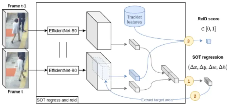
Fig. 1. For each current frame, all targets go through a SOT to (i) predict their displacement w.r.t their previous position, (ii) extract the target-specific embedding from the EfficientNet output feature map based on the predicted position offset, and (iii) compare it with the appearance embedding of the candidate tracklet and produce a reidentification score.

D. Tracklets management strategy

Updating the state of a tracklet i.e., its position, appearance, and managing its birth, death, inactivity is handled in various ways in the literature. Usually, position and appearance are replaced by the associated detections [12], [15], [19]. It is then common to consider a track active when it is assigned an incoming detection, and inactive when not associated in order to kill targets lost for too long [9], [11], [15]. By considering unfiltered detector inputs and setting up a balanced strategy, we propose to either rely on detector or tracker and keep targets active depending on the confidence of each element.

III. METHODOLOGY

Even if almost 60% of the MOT17 submissions use CNNs for reidentification, only a few take advantage of CNN-based techniques for predicting targets position. Above all, despite the performance shown by SOT within MOT [9], no previous work has been done to integrate a single light-weight CNN for both predicting targets position and producing reidentification features at once in this realtime multi-target context.

Furthermore, is it common to give full trust to the detector when it comes to updating tracklets status after the tracklet-detection association phase; we put forward a balanced strat-egy allowing confident trajectories to keep living even when faced with spurious detections. We integrate multiple cues in our general framework, analyzed through an ablation study in sectionV.

A. Position prediction

1) Single Object Track’n’Reid for MOT: We incorporate SOT-dedicated trackers in a multi-object framework by en-riching them with identity awareness. Figure 1 describes how tracklets update their position and similarity scores at every timestep t, all-at-once through a single CNN, before being faced with incoming detections. This tracklet prediction consists of three main parts:

• High-speed joint feature extraction. We take a patch from both previous and current frames, centered on the current target location at t − 1. We call them target and search region patches. They are enlarged by a context

factor k as in [4], resized to [256 × 128] and fed to a siamese EfficientNet-B0 backbone for feature extraction, which shares its weights across both inputs.

• Motion prediction branch. On one side, we get two output volumes from EfficientNet corresponding to target and search patches inputs. We reduce the outcoming channel dimensions from 1280 to 128, apply average pooling and concatenate outputs to finally send them to a 4-neuron 1 × 1 output layer predicting a ∆(x, y, w, h) shift vector, relatively to the search region width w and height h. It is illustrated by the grey branch on figure 1. • Similarity branch. On the other side, we compute the cosine similarity between the current and predicted target appearance features. The appearance feature map is sliced from the feature extractor output volume of the search area, based on the predicted coordinate shift. It is then average pooled and transformed via 1 × 1 convolutions to finally calculate the cosine similarity with the target feature model. It is illustrated by the blue branch on figure 1.

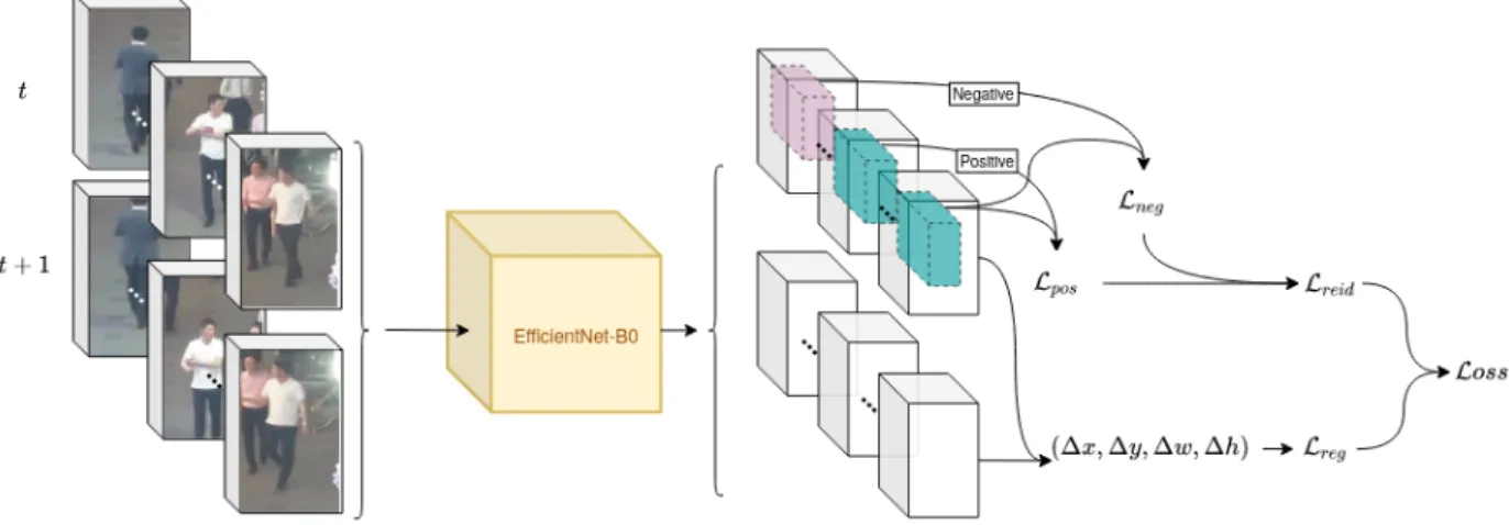
2) Multi-task learning: In order to perform joint task learn-ing, the network is trained with a combined regression/reid loss. As shown in figure2, during training we feed the siamese network with SOT-dedicated inputs i.e., target and search patches at time t and t + 1, and batch multiple examples together. In parallel, we use them to construct positive and negative pairs later in the similarity branch. These pairs are sliced from the feature map centers at time t, average pooled, and used to calculate cosine similarity loss functions Lpos and Lneg where positive (resp. negative) pairs scores must be close to 1 (resp. −1). The reidentification loss Lreid is the sum of cosine embedding losses for positive and negative pairs (Lpos+ Lneg).

Regarding the position regression part of the network, both t and t + 1 feature extractor entire outputs are average pooled, concatenated and convolved to predict an (x, y, w, h) offset which is compared to the groundtruth via L1 loss and stored in Lreg. In the end, the final loss can be written as in equation1:

L = Lreg+ 1

2 (Lpos+ Lneg) (1) B. Tracklet-detection association

As mentioned in section II-C, at every online timestep each upcoming detection must either be associated to an existing trajectory, lead to a track birth or potentially be discarded. It is usually done by calculating an association cost between each possible detection-tracklet matching. The resulting cost matrix is then passed to a cost minimization solver, classically a Hungarian algorithm [20]. Different cues are usually considered to calculate the association cost, and the impact of each one is here explored with an ablation study in section V:

1) Intersection over Union: The overlap between bounding boxes IoUD,T is a major discriminatory measure but it can lead to identity switches when two targets are close to each other.

Fig. 2. Joint all-in-one training process of the full siamese SOT for regression and reidentification. For each target, two inputs at t and t + 1 are fed to an EfficienNet backbone for feature extraction. Multiple identities are batched together; we combine them to contruct positive and negative pairs in the batch. The feature extractor output volumes are used (i) in depth to extract sliced positive and negative pairs and calculate their cosine distance losses Lpos and

Lneg, and (ii) between t and t + 1 to calculate the image coordinates displacement, thus the regression loss Lreg. All losses are combined to produce a

unique final loss.

2) ReID: To overcome this issue, we also apply the similar-ity branch of our network to the detections and compare their embedding with the targets ones to get the cosine similarity cosD,T.

3) Detection score: We use the detector confidence scores Dcf lock, stock and barrel, arguing that based on good prior detections like SDP’s, the use of raw inputs without filtering, altering or discarding information can be precious knowledge. 4) Target confidence: At every timestep, each tracklet up-dates an inner confidence score Tcf detailed in the next section and inspired by LSST [9].

We bring the [−1, 1] cosine similarity distance for reiden-tification back between 0 and 1 in order to finally multiply together [0, 1] range elements and get a normalized overall score. Combined together, we end up with a similarity score SD,T between a detection D and a tracklet T , thus an association cost CD,T defined by equation2.

SD,T = Tcf× IoUD,T × cosD,T × Dcf CD,T = 1 − SD,T

(2) C. Tracklets management strategy

At each frame, every tracklet updates its appearance embed-ding, confidence score and state depending on data association and prediction uncertainty. The integration of these elements in the overall multi-track algorithm is detailed at the end of the section.

1) Historical appearance embedding: As shown in figure1, every tracklet compares the appearance sliced from the SOT-predicted position with its current appearance embedding. In order to avoid drifting, we only update these visual features when a match is found with a detection. This way, the tracklet reidentification confidence score states how much the prediction looks like the last associated detection.

Numerous approaches [9], [11], [15] use a list of the last matched appearance embeddings to overcome the issue of storing altered features e.g., if a target happens to be occluded

or suddenly changes under varying lighting conditions, the appearance embedding is not crushed by the alteration and still has a stable representation in memory. The similarity score between a detection and a track embedding is therefore defined as a combination of the similarity scores among this list of stored features. Despite the aforementioned interest of this strategy, comparing tens of vectors in a combinatorial way e.g., in [11], [15], is time-consuming. As formulated in equation 3, we address this issue by storing only one appearance embedding Tf eat for each track and updating it with the associated detection embedding Df eatweighted by a temporal memory factor τm. This way, the comparison is fast and we still keep trace of appearance history.

Tf eat= (1 − τm) × Tf eat+ τm× Df eatif match(D, T ) (3) 2) Tracklet confidence multi-score: In the vein of LSST [9], the tracklet confidence score formulated by equation4 alterna-tively integrates information about track prediction or matched detection depending on the association phase outcome:

Tcft= ((T_cft−1+IoUD,T×cosD,T×Dcf) 2 if match(D, T ) Tcft−1× decay × Treid k , otherwise (4)

• if a match is found between a detection D and a tracklet T , the tracklet updates its previous confidence score Tcft−1 with the product of the detection score, their

overlap and their similarity score. Dividing the result by 2 as in equation4brings the score back to a [0, 1] range; • if no match is found, we update the confidence score with a decay factor and the track reidentification score between prediction and current appearance features. As in [9], an exponent k is applied to negatively impact uncertain tracks.

Where LSST only integrates IoU, we benefit from richer information like appearance similarity of match, prediction and detection confidence measure.

3) Status update: The tracklet-detection association phase is not enough: it does not handle non-detections, and occlu-sions can still lead to inconsitency in tracklets. A mechanism is put in place to deactivate ambiguous trajectories and maintain alive non-associated tracks based on their SOT prediction confidence, thus finding the right balance between detection and tracking instead of only relying on the detector knowledge. The last step after prediction and data association then consists in updating the tracks as follows:

a) Active/Inactive flag:

• if a detection leads to track birth or is associated to an existing trajectory, this tracklet is set to active mode; • if a track was active at time t − 1 but is not assigned

a detection at time t, it shifts to inactive mode only if the track confidence score Tcft drops below a certain

threshold τactive. This way, we also give trust to the tracker knowledge instead of only relying on the detector expertise as it is usually done;

• after data association, we perform Non-Maximum-Suppression based on all targets confidence score with an IoU threshold τnms to filter out occluded trajectories and transit them towards inactive mode.

A tracklet position is updated during prediction phase only if the track is active. This way, a drifting SOT will not stick to occluders or wander around when the target has exited the frame.

A two-step process is commonly applied during data associ-ation [11], [15] and consists in matching detections with active trajectories before looking at inactive ones. By using tracking confidence in the tracklet-detection assignment, inactive tra-jectories will implicitly lower the cost and be assigned after active ones. We thus apply a single-pass matching process to save processing time.

b) Birth/Death management:

• when a detection with a score Dcf is not assigned to any existing tracklet, it leads to the creation of a trajectory, only if Dcfis above a certain threshold τinit. Even if later in the association part we do consider every detection without any filtering, this threshold is important to avoid creating spurious false positive tracklets in the beginning and be confident about the appearance and position the SOT will have as a starting point;

• at birth, every tracklet is considered as a tentative. It is regarded as confirmed only after ninit associations in a row. In this way, flickering detections e.g., two low confidence detections interleaved with a non-detection will not end up in the confirmation of a false track; • if a track has not been associated to a detection ninit

consecutive times at birth, or if it has been inactive over than nwait successive frames, it gets killed. To this end, a counter Tcounter is incremented as long as the tracklet remains inactive, and reset to 0 when a detection is matched. These two strategies are already used in the literature [15] and are efficient at reducing the number of false positives and identity switches.

All put together, the elements of prediction, data association and tracklets update can be summarized by Algorithm 2.

Algorithm 2 Overall tracking process

1: Inputs:

• {It}0≤t≤N −1a set of N consecutive images

• {Dt}0≤t≤N −1a set of N detection pools for each image t

2: Output: {T_tj}0≤j≤M −10≤t≤N −1 a set of M distinct tracklets for each

timestep t

3: T0← ∅

4: for Dt, It∈ zip(D, I) do

. Detections feature extraction 5: Ct← crop(Dt, It)

6: Ft← backbone(Ct)

7: Dtf eat ← reid_branch(Ft[Dt]) . Fig.1

. Targets prediction 8: if Tt−16= ∅ then 9: C[t−1,t]← crop(Tt−1, [It−1, It]) 10: F[t−1,t]← backbone(C[t−1,t]) 11: X ← SOT_branch(Fˆ t−1, Ft) . Fig.1 12: f eat ← reid_branch(Fˆ t[ ˆX]) 13: if Tt−1 is active then Tt← ˆX 14: else Tt← Tt−1

15: Tt_reid ← cos(Tf eat,f eat)ˆ

. Tracklet-detection association

16: SD,T ← score(Dt, Tt) . Eq.2

17: CD,T ← mask_to_inf((1 − SD,T), τIoU, τreid)

18: matches ← hungarian(CD,T)

. Tracklets update 19: for (Dtp, Ttq) ∈ matches do

20: Ttq ← Dtp, active . Update position & status

21: Tt_qcounter ← 0

22: Tt_qreid ← cos(Tt_qfeat, Dt_pfeat)

23: Tt_qfeat ← update(Dt_pfeat) . Eq.3

24: Tt_qcf ← update(Dtp) . Eq.4

25: Dt← Dt− Dtp

26: if Dt6= ∅ and Dtcf ≥ τinit then . Tracks birth

27: Tt← Tt∪ Dt

28: for Tti∈ matches do/ . Unmatched tracks

29: Tt_icf ← update() . Eq.4

30: if Tti is active and Tticf ≥ τactivethen

31: Tti← active

32: else Tti ← inactive

33: if Tti is tentative then

34: Tt← Tt− Tti . Delete ”baby” tracks

35: indices ← NMS(Ttcf, τnms) . Deal w/occlusions

36: Tt[indices] ← inactive

37: for all Tt do

38: if Tt is inactive then Tt_qcounter+ = 1

39: if Tt_qcounter ≥ nwaitthen

40: Tt← Tt− Ttq . Delete old inactive tracks

IV. IMPLEMENTATION AND LEARNING PHASE

All evaluations are performed on an Intel Xeon E5-1620v4@3.50Ghz x 8 CPU with 16GB RAM and a NVIDIA Titan X (Pascal) GPU, with Python and Torch.

A. Dataset

We evaluate ourselves on the MOT17 benchmark [1]. It consists of 14 pedestrian static and moving video sequences taken from different views, cut in half for training and testing. Among the whole dataset, 1280 distinct trajectories have been annotated following a strict protocol, and the output of three different frame-by-frame detectors are given as raw inputs to solve the multi-tracking task. As described in section I, we evaluate ourselves on the SDP detector and compare our results with the other MOT17 submissions for this detector. B. Training data generation

1) SOT: As described in figure 2, we construct pairs of image crops centered on targets at time t and cropped at the same location at time t + 1. In order to get variability within the identities, we set to 3 the number of examples per track to generate i.e., for the same identified target, we take 3 different crops at different times and retrieve their corresponding t + 1 crops. Within the same batch, we also retrieve 5 more identities with their 3 examples.

Because the displacement of a target between two succes-sive frames is very small – thus close to zero, we also perform data augmentation by randomly shifting the crops taken from t+1 [4]. We end up with multiple [t, t+1] pairs for each target, the first one being the real example, the others corresponding to the shifted augmented ones.

In the end, we have as input to the network a batch of 72 examples of t and t + 1 crops (6 identities, 3 examples per identity, 1 real t + 1 and 3 augmented ones).

2) Similarity learning: Positive and negative pairs are built from the 72 crops at time t available in a training batch. We construct 540 combinations of {anchor, positive, negative} triplets allowing us to calculate the positive cosine embedding loss for the {anchor, positive} pairs and negative cosine embedding loss for the {anchor, negative} pairs, the two categories being equally balanced.

C. Hyperparameters

All training parameters like context and scale factors or solver are the same as in [4]. The thresholds and tuned parameters of the overall process formulated in sectionIIIare optimized with SMAC [21] on training sequences and floored to the closest decimal value during inference. For clarity, we gather these hyperparameters, their values and description in TableI.

V. EVALUATIONS AND ASSOCIATED ANALYSIS

A. Metrics

As it is done in the benchmark, we evaluate our tracker with the CLEARMOT metrics [22]: false positives FP, false negatives FN, identity switches IDS and more importantly the multi object tracking accuracy MOTA which combines together these metrics and gives a relevant insight on the over-all tracking performance. We also discuss time consumption performance i.e., the number of frames per second FPS.

TABLE I

HYPERPARAMETERS USED IN THE OVERALLMOTALGORITHM. Param. Value Description

τinit 0.5 Detection threshold for track birth

τnms 0.5 IoU threshold for NMS

τIoU 0.25 IoU threshold for possible data association

τreid 0.35 Similarity threshold for possible data association

τm 0.8 Temporal memory weight factor for feature update

τactive 0.5 Tracklet confidence threshold to keep active

decay 0.98 Tracklet confidence decay if not matched

k 2 Confidence exponent used during update if not matched ninit 3 Time before a track gets confirmed

nwait 20 Inactive patience before killing a track

TABLE II

ABLATION STUDY SHOWING THE IMPACT OF THE TRACKLETS MANAGEMENT STRATEGY ELEMENTS FORMULATED IN SECTIONIII. (A) (B) (C) (D) (E)

IoU ReID Classif. Keep Init FP ↓ FN ↓ IDS ↓ MOTA ↑

X 4259 34314 1309 64.49 X X -1014 +1004 -267 +0.24 X X X +1693 -1187 -220 -0.25 X X X -1152 +994 -307 +0.41 X X X X +191 -802 -263 +0.78 X X X X X -462 -325 -297 +0.96 B. Ablation study

The following ablative analysis has two important purposes: • confirm the added value of each single component de-scribed in sectionIIIduring tracklet-detection association (Eq. 2) and tracklet confidence score update (Eq. 4); • find the optimal tracking performance configuration. As described in sectionIII, we use different information for calculating both tracklet-detection association costs and track-let confidence scores: intersection over union (A) IoU, rei-dentification measure of the prediction/association (B) ReID, detection confidence score (C) Classif. When we say that one of them is not used, we mean both in the association cost and tracklet confidence score. We also analyze the impact of two tracklets management strategies: keeping a confident track active even if it is not associated to any detection ((D) Keep) and confirm a track only if associated to a detection ninit times in a row after its creation ((E) Init).

In table II, IoU is used as a baseline to calculate the gain of each element.

1) Wait at init: (A+E) Waiting for multiple associations before confirming a tracklet shows a gain to the baseline of +0.24 on the MOTA. Looking at table II, we note that it is mainly due to the gain over identity switches which can be explained by the false positives drop down leading to less ambiguous situations.

2) Complementary ReID and keep active: An interesting outcome lies in the use of reidentification and keep active strategy separately and then in a complementary way.

(A+B+E) On the one hand, we note that reidentification alone with IoU and initial patience simultaneously improves false positives and identity switches, thus following the ex-pected behavior when adding appearance information as extra

TABLE III

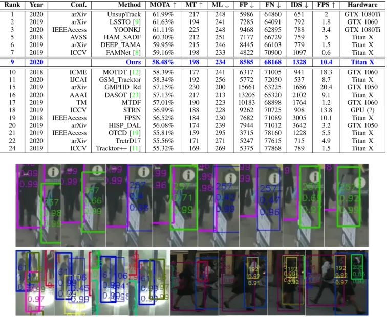
COMPARISON OF ONLINECNN-BASEDMOT17SUBMISSIONS ON THE TEST SET FOR THESDPDETECTOR.

Rank Year Conf. Method MOTA ↑ MT ↑ ML ↓ FP ↓ FN ↓ IDS ↓ FPS ↑ Hardware

1 2020 arXiv UnsupTrack 61.99% 217 248 5986 64860 651 2 GTX 1080Ti

2 2019 arXiv LSSTO [9] 61.63% 194 241 7285 64091 792 1.8 GTX 1060

3 2020 IEEEAccess YOONKJ 61.11% 225 248 9468 62895 788 3.4 GTX 1080Ti

5 2018 AVSS HAM SADF 60.30% 212 251 7177 66729 759 5 Titan X

6 2019 arXiv DEEP TAMA 59.95% 215 246 8445 66103 779 1.5 Titan X

7 2019 ICCV FAMNet [8] 59.16% 198 233 4822 70900 1097 0.6 Titan X

9 2020 Ours 58.48% 198 234 8585 68168 1328 10.4 Titan X

10 2018 ICME MOTDT [12] 58.39% 177 241 6317 71005 941 18.3 GTX 1060

11 2020 IJCAI GSM Tracktor 58.34% 192 256 5772 72050 537 8.7 Titan X

15 2019 arXiv GMPHD Rd 57.15% 230 200 15661 63225 1686 20.4 GTX 1050

16 2020 AAAI DASOT [23] 57.13% 217 213 13205 65320 2102 9.1 Titan X

17 2019 TM MTDF 57.01% 190 223 10183 68898 1764 1.2 GTX 1060

18 2019 ICCV STRN 56.99% 188 228 9262 70725 908 13.8 GPU (?)

19 2018 IEEEAccess FPSN 56.52% 184 230 7682 71089 3005 10.1 Titan X

20 2019 arXiv HISP DAL 56.08% 174 239 7944 71012 3642 3.2 GTX 1050

21 2019 IEEEAccess OTCD [19] 55.81% 159 295 3715 78160 1228 5.5 Titan X

22 2020 arXiv TrctrD17 55.56% 171 271 5247 77615 715 4.9 Titan X

24 2019 ICCV Tracktor++ [11] 55.32% 169 269 5375 77868 789 1.5 Titan X

Fig. 3. Qualitative examples of our framework. Thick colored: identified tracklets associated with a detection. Thin blue: non-associated tracks being kept active because of their confidence score. Thin yellow: inactive tracks. In each box, the first number is the target identity, the second is the detection confidence score and the third is the tracklet reidentification score with the associated detection or predicted position. The first row and left half of the second one illustrate cases where keeping a confident track active pays off under scene occlusions. The right half of second row shows a type of identity switch our framework still struggles with. For better viewing, a video is provided as supplementary material.

knowledge. However, because this strategy filters out more tracklets, it still suffers from high false negatives.

(A+D+E) On the other hand, keeping confident tracklets active even when no detection was assigned, and without any reidentification insight, tends to inevitably increase false positives – symmetrically decrease false negatives, and be less efficient on identity switches than with (A+E) configuration.

(A+B+D+E) As highlighted in tableII, using both reidenti-fication and keep active in a complementary fashion allows to both lower false negatives and identity switches while maintaining false positives relatively low. In the end, when (A+D+E) impacts MOTA negatively and (A+B+E) shows a

small gain of 0.41%, combining them leads to a 0.78% gain. 3) Benefiting from raw detector inputs: (A+B+C+D+E) Adding detector confidence scores into the pipeline leads to a global gain of 0.96% on the MOTA, and 0.18% relatively to the previous configuration (A+B+D+E). In tableII, we observe a rebalance on each type of error but more specifically on the false positive part, confirming the fact that tracker and detector are complementary mechanisms and can both benefit from each other.

Not illustrated in this paper, we also led experiments apply-ing a threshold on upcomapply-ing detection scores to only consider trusted ones, it decreases the MOTA and confirms our first

belief of tracker-detector complementarity.

4) Substantial gains: The gains presented in this ablation study are substantial regarding the challenge: comparing our method relatively to the other approaches in the literature (tableIII), we note that improving our method by almost +1.0 in MOTA led to a 6 place jump forward in the overall ranking. Figure 3 shows qualitative examples of our framework. The first row as well as the first half of second row show cases benefiting from our keep active strategy described in sectionIII-C3. Looking at tracklets 257 and 106, we observe a balance between detector and tracker, where detection con-fidence scores start to drop under occlusions with objects in the scene but where tracks are still being kept active thanks to a reidentification score (hence a confidence score) remaining high. The tracker fulfils its catch-up role when the detector fails.

However, when total occlusions occur between targets (pur-ple and blue targets on the right half of second row), the system deactivates the occluded track and struggles associ-ating it correctly when it appears again. As illustrated in the second thumbnail, this is mainly because before deactivating the background track, a large portion of the targets gets involved in the two appearance feature vectors, leading to miss-reidentification.

C. MOT17 evaluations

In tableIIIwe compare our framework to the literature on the MOT17 test set with SDP detections. For fair comparison (especially on the execution time), we only show the CNN-based approaches, whether they use deep networks for position prediction or for reidentification. In any case, they generally perform better than other methods, with only one or two exceptions.

A few approaches integrating SOT for position prediction are designed concurrently with our work [9], [23], but we still present an original all-in-one architecture which obviously outperforms recent state-of-the-art MOTA performance on the benchmark [11], [17]. Beside tracking performance, we put forward a ×2 to ×17 gain in speed w.r.t. the the MOTA top-ranked CNN-based approaches, putting our method on the path towards realtime constraints for embedded applications.

VI. CONCLUSION AND FUTURE WORKS

In this work, we put forward an original architecture inte-grating a jointly trained all-in-one single light-weight siamese CNN for both tracklet position prediction and reidentification in a multi-object tracking context. We present a novel training data generation and tracklet management strategy for this purpose and show state-of-the-art results on the well-known MOT17 benchmark, in terms of both tracking results and speed.

Due to the success of recent single object tracking work using intercorrelation inside their network [5], [24], [25], we aim at improving our architecture with such techniques but also find an in-between strategy within the appearance feature management strategy to deal with identity switches induced by full target-to-target occlusions.

REFERENCES

[1] A. Milan et al., “MOT16: A benchmark for multi-object tracking,” 2016. [Online]. Available:http://arxiv.org/abs/1603.00831 1,2,6

[2] Y. Taigman et al., “DeepFace: Closing the gap to human-level perfor-mance in face verification,” IEEE Conference on Computer Vision and Pattern Recognition (CVPR), 2014.1

[3] F. Schroff et al., “FaceNet: A unified embedding for face recognition and clustering,” IEEE Conference on Computer Vision and Pattern Recognition (CVPR), 2015.1

[4] D. Held et al., “Learning to track at 100 fps with deep regression networks,” in European Conference on Computer Vision (ECCV), 2016.

1,3,6

[5] B. Li et al., “High Performance Visual Tracking with Siamese Region Proposal Network,” IEEE Conference on Computer Vision and Pattern Recognition (CVPR), 2018.1,8

[6] Y. Xu et al., “SiamFC++: Towards Robust and Accurate Visual Tracking with Target Estimation Guidelines,” AAAI Conference on Artificial Intelligence, 2020. 1

[7] M. Kristan et al., “A novel performance evaluation methodology for single-target trackers,” IEEE Trans. Pattern Anal. Mach. Intell., 2016.1

[8] P. Chu and H. Ling, “Famnet: Joint learning of feature, affinity and multi-dimensional assignment for online multiple object tracking,” in IEEE International Conference on Computer Vision (ICCV), 2019. 1,

2,7

[9] W. Feng et al., “Multi-Object Tracking with Multiple Cues and Switcher-Aware Classification,” 2019. [Online]. Available:http://arxiv. org/abs/1901.061291,2,3,4,7,8

[10] M. Tan and Q. V. Le, “Efficientnet: Rethinking model scaling for convolutional neural networks,” in International Conference on Machine Learning (ICML), 2019. 1

[11] P. Bergmann et al., “Tracking without bells and whistles,” in 2019 IEEE International Conference on Computer Vision (ICCV), Seoul, Korea, Oct. 2019. 1,2,3,4,5,7,8

[12] L. Chen et al., “Real-Time Multiple People Tracking with Deeply Learned Candidate Selection and Person Re-Identification,” IEEE In-ternational Conference on Multimedia and Expo (ICME), 2018.1,2,3,

7

[13] A. Bewley et al., “Simple online and realtime tracking,” in IEEE International Conference on Image Processing (ICIP), 2016.2

[14] R. Sanchez-Matilla et al., “Online multi-target tracking with strong and weak detections,” in European Conference on Computer Vision Workshop (ECCVW, 2016.2

[15] N. Wojke et al., “Simple online and realtime tracking with a deep asso-ciation metric,” in IEEE International Conference on Image Processing (ICIP), 2017. 2,3,4,5

[16] “Learning discriminative appearance models for online multi-object tracking with appearance discriminability measures,” 2020.2

[17] J. Zhu et al., “Online multi-object tracking with dual matching attention networks,” in European Conference on Computer Vision (ECCV, 2018.

2,8

[18] S. Karthik et al., “Simple unsupervised multi-object tracking,” 2020. [Online]. Available:http://arxiv.org/abs/2006.02609 2

[19] Q. Liu et al., “Real-time online multi-object tracking in compressed domain,” IEEE Access, 2020. 3,7

[20] J. Munkres, “Algorithms for the assignment and transportation prob-lems,” Journal of the Society for Industrial and Applied Mathematics, vol. 5, no. 1, 1957.3

[21] F. Hutter et al., “Sequential model-based optimization for general algorithm configuration,” in International Conference on Learning and Intelligent OptimizatioN (LION), 2011.6

[22] K. Bernardin and R. Stiefelhagen, “Evaluating multiple object tracking performance: The clear mot metrics,” EURASIP Journal on Image and Video Processing, vol. 2008, 01 2008.6

[23] Q. Chi et al., “Dasot: A unified framework integrating data association and single object tracking for online multi-object tracking,” AAAI Conference on Artificial Intelligence (AAAI), 2020.7,8

[24] Z. Zhu et al., “Distractor-aware siamese networks for visual object track-ing,” in European Conference on Computer Vision (ECCV), September 2018.8

[25] B. Li et al., “Siamrpn++: Evolution of siamese visual tracking with very deep networks,” in IEEE Conference on Computer Vision and Pattern Recognition (CVPR), 2019.8