Algorithmic aspects of high speed switching

Algorithmic Aspects of High Speed Switching

by

Saadeddine Mneimneh

Submitted to the Department of Civil and Environmental Engineering

in partial fulfillment of the requirements for the degree of

Doctor of Philosophy

at the

MASSACHUSETTS INSTITUTE OF TECHNOLOGY

May 2002

EJUwg ooJ

©

_{Massachusetts Institute of Technology 2002. All rights reserved.}

Author ...

Department of Civil and Envifonmental Engineering

May

10, 2002

Certified by.

...

Kai-Yeung Siu

Associate Professor

Thesis Supervisor

Accepted by...

Oral Buyukozturk

Chairman, Department Committee on Graduate Students

MASSACHUSETTS INSTITUTE OF TECHNOLOGY

Algorithmic Aspects of High Speed Switching

by

Saadeddine Mneimneh

Submitted to the Department of Civil and Environmental Engineering on May 10, 2002, in partial fulfillment of the

requirements for the degree of Doctor of Philosophy

Abstract

A major drawback of the traditional output queuing technique is that it requires a switch speedup of N, where N is the size of the switch. This dependence on N makes the switch non-scalable at high speeds. Input queuing has been suggested instead. The introduction of input queuing creates the necessity for developing switching al-gorithms to decide which packets to keep waiting at the input, and which packets to forward across the switch. In this thesis, we address various algorithmic aspects of switching.

We prove in this thesis, that many of the practical switching algorithms still require a speedup to achieve even a weak notion of throughput. We propose two switching algorithms that belong to a family to which we refer in this thesis as priority switching. _{These two algorithms overcome some of the disadvantages in existing} priority switching algorithms, such as the excessive amount of state information that needs to be maintained. We also develop a practical algorithm that belongs to a family to which we refer in this thesis as iterative switching. This algorithm achieves high throughput in practice and offers the advantage of not requiring more than one iteration, unlike other existing iterative switching algorithms which require multiple iterations to achieve high throughput. Finally, we address the issue of using switches in parallel to accommodate for the need of speedup. We study two settings of parallel switches, one with standard packet switching, and one with flow scheduling, in which flows cannot be split across multiple switches.

Thesis Supervisor: Kai-Yeung Siu Title: Associate Professor

This research was supported by: NSF Award 9973015 (chapters 2, 3, and 6), Alcatel Inc. (chapter 4), and Tellabs Inc. (chapter 5, patent filed).

Acknowledgments

The acknowledgments section is an important part of a Ph.D. thesis because, most

of the times, it comes out to be sincere. It contains names of people and pointers to

the social aspect of the Ph.D. experience. I think a collection of acknowledgements out of many Ph.D. theses may reflect a complete picture of the human social Ph.D. experience.

I defended my thesis few weeks ago, and at the end of my defense, I felt that I was leaving something behind, and I couldn't just stop without thanking a number of people. I said few words. I will try to reproduce these words here because they summarized my MIT social Ph.D. experience.

I will traditionally start by thanking my advisor Sunny Siu. However, my thanking to him is non-traditional, for allowing me towards the ends of my Ph.D., to waste time and do some research, while physically away from MIT in Dallas with my wife, at a time when my wife and I both needed to be close.

I thank Steve Lerman for helping me in the beginnings and encouraging me to apply to MIT. Needless to say, coming to MIT changed my life (for the better, or at least that's what is apparent so far).

I thank Kevin Amaratunga for accepting to serve as a member on my Ph.D. committee in its first meeting on a very short notice (and for staying later on).

I thank Jud Harward for all the fights that we had when we worked together over a period of 4 years because I learned a lot from him.

I thank Cynthia Stewart for facilitating all the departmental logistics and for not going after me and pushing me to fill out the paper work (as she does with other students).

I thank all my MIT teachers for whom I owe most of my knowledge. I mention Arvind, David Gifford, Michael Sipser, Dan Spielman, David Karger, Nancy Lynch, Charles Rhors...

I thank all my fellow lebanese/arab students at MIT who created for me an ap-propriate microcosm and provided me with a sense of belonging. They shaped and

refined my thoughts through many cultural/political events that we organized to-gether, and through many discussions that never ended. At MIT, we implemented together the "thinking outside the box" when all of us with common backgrounds met on an uncommon ground. The maturity of intellect that I gained from interac-tions with my lebanese/arab friends makes this document the least important part of my Ph.D. experience (speaking of this document, my friends actually helped me re-produce this document when my laptop computer was stolen few days ago with everything on it and no backup). I would like to mention some names here: Issam Lakkis (aka the Poet), Louay Bazzi (as of today, the smartest person at MIT), Ra-bih Zbib (aka the expert on foreign affairs), Nadine Alameh, Hisham Kassab, Dina Katabi, Omar Baba, Fadi Karameh and Assef Zobian (aka the druze connection), Ibrahim Abou-Faycal (aka "al-za3eem" i.e. the leader, but no one really believes that), Jean-Claude Saghbini (aka the sailor), Mahdi Mattar (aka "al-mountazar" i.e. the expected one), Walid Fayad (aka "malek el..." i.e. the king of...), Ziad Younes, Mona Fawaz, Alan Shihadeh, Husni and Khaled Idris (aka the Idris brothers), Maya Said, Yehia Massound, Karim Hussein, Maysa and Ziad Sabah, Hassan Nayfeh, Bilal Mughal, Richard Rabbat, Ahmad Kreydiyeh (aka kreydiyeh), Maya Farhoud, Ziad Zak, Ziad Ferzly, Bassam Kassab, Danielle Tarraf, Joe Saleh...

I THANK my parents Salma and Sami and my family for helping me come to MIT, for supporting me throughout the years (emotionally and financially), for calling me on the phone more than 375 times so far, and for doing every possible thing to make me happy at the cost of loosing my presence as one of the family. I THANK them for relieving me from my responsibilities towards the family, and for handling my absence for 7 years. There is nothing I can do to return their sacrifice.

I thank my wife Nora Katabi for helping me through the stressful times, for changing my life to the better, and for being part of it. I thank her for giving me the possibility to wake up every day and look at a face that I like (something I could not achieve by just looking at the mirror), and for giving me hope in life.

I also thank Farhoud, Farkoush, Saeid, and Arnoub el Hazz. Finally, I thank Allah (i.e. God) for many things...

To my now bigger Family...

I LOVE you.

Second dedication:

To Cambridge, Boston, Charles River, and MIT Steps...

Contents

1 Introduction

1.1

Output Queuing . . . .

.

1.2

The Speedup Problem . . . .

1.3

Input Queuing . . . ..

1.3.1

HOL Blocking . . . .

1.3.2

Formal Abstraction . . . .

1.4

Input-Output Queuing . . . .

1.5 Traffic Models . . . .

1.5.1

SLLN Traffic

. . . .

1.5.2

Weak Constant Burst Traffic . .

1.5.3

Strong Constant Burst Traffic .

1.6

Guarantees

. . . .

1.6.1

Throughput . . . .

1.6.2

Delay . . . .

1.7

Existing Switching Algorithms . . . . .

1.7.1

Maximum Weighted Matching .

1.7.2

Priority Switching Algorithms .

1.7.3

Iterative Switching Algorithms .

1.8

Thesis Organization

2 Some Lower Bounds on Speedup

2.1

Traffic Assumptions...

....

. . . .

.

2.2

Priority Scheme ...

17

18

19

19

20

21

22

24

24

25

26

27

27

29

. . . .

29

. . . .

30

31

33

35

39

2.3 Lower Bounds . . . . 42

2.3.1 Output Priority Switching Algorithms . . . . 43

2.3.2 Maximum Size Matching . . . . 47

2.3.3 Maximal Matching . . . . 47

2.3.4 Input Priority Switching Algorithms . . . . 48

2.4 Summary . . . . 57

3 Two Priority Switching Algorithms 59 3.1 Earliest Activation Time . . . . 60

3.2 Latest Activation Time . . . . 62

3.3 Implementation Issues . . . . 64

3.3.1 Time and Space Complexity . . . . 65

3.3.2 Communication Complexity . . . . 65

3.4 Summary . . . . 66

4 An Iterative Switching Algorithm 69 4.1 The ir-RCA Switching Algorithm . . . . 71

4.2 Stable Priority Scheme r . . . . 73

4.3 Bounded Bypass Priority Scheme 7 . . . . 76

4.4 Theoretical Results . . . . 78

4.4.1

SLLN Traffic . . . .

78

4.4.2 Weak Constant Burst Traffic . . . . 79

4.4.3 Strong Constant Burst Traffic . . . . 79

4.5 Experimental Results . . . . 80

4.5.1 Standard Switch . . . . .. . . . . 82

4.5.2 Burst Switch . . . . 83

4.5.3 Multiple Server Switch . . . . 84

4.6 Summary . . . . 87

5 Switching using Parallel Switches with no Speedup 89 5.1 Motivation . . . . 90

5.2

The Parallel Architecture . . . .

5.2.1

Segmentation . . . .

5.2.2

Rate Splitting . . . .

5.2.3

Basic Idea . . . .

5.3

The Approach . . . .

5.3.1

Demultiplexer Operation . . . .

5.3.2

Switching Operation . . . .

5.3.3

Multiplexer Operation . . . .

5.3.4

Supporting Higher Line Speeds

.

. . .

5.4 Summary . . . .

6 Scheduling Unsplittable Flows Using Parallel

6.1

The Problem . . . .

6.2

Theoretical Framework . . . .

6.3

Maximization . . . .

6.4 Number of Rounds . . . .

6.5

Speedup.. . .

...

6.6

Summary . . . .

7 Conclusion

7.1

Some Lower Bounds on Speedup . . . .

7.2 Two Priority Switching Algorithms . . . .

7.3

An Iterative Switching Algorithm . . . .

7.4

Switching Using Parallel Switches . . . .

7.5

Unsplittable Flows . . . .

Switches

92

94

95

96

98

98

103

114

117

119

121

123

124

125

130

133

137

139

140

141

141

142

142

List of Figures

1-2

1-3

1-4

1-5

1-6

1-7

2-2

2-3

Output queued switch . . . .

Input queued switch . . . .

Input queued switch with VOQs

. . . ..

Formal operation of the input queued switch Input-Output queued switch with VOQs . . . . Priority switching algorithms . . . . Iterative switching algorithms . . . . The q-Adversary . . . .

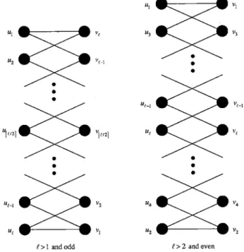
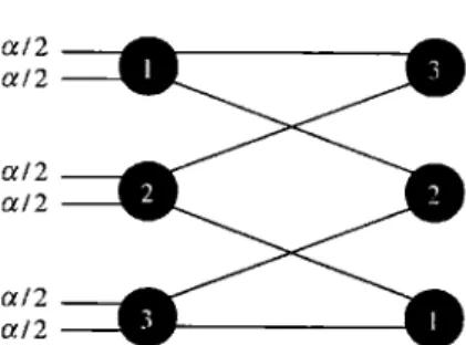
tsymmetric cycles . . . . The 3-symmetric

#-Adversary

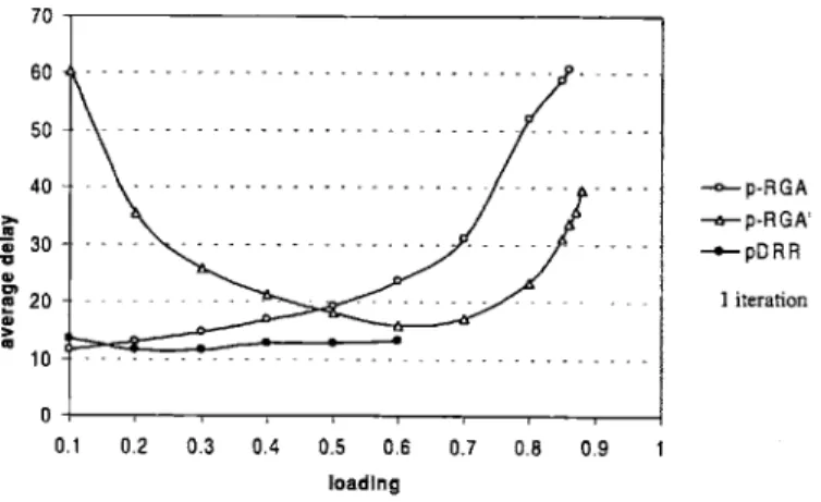
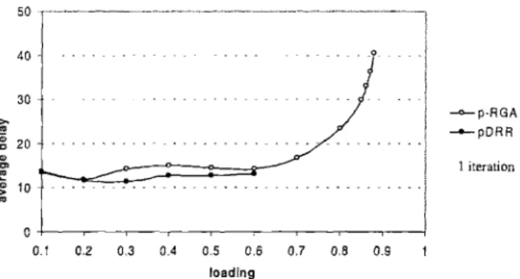
4-1 The 7r-RGA switching algorithm . . . .

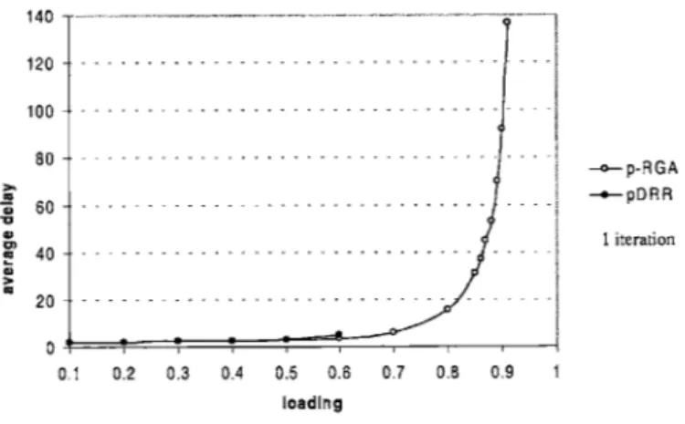
4-2 'r-RGA and pDRR with one iteration for B

=

1 . . . .

4-3 7r-RGA' and pDRR with one iteration for B

256 . . . .

4-4 Modified 7r-RGA' and pDDR with one iteration for B

=

256...

4-5 VOQ activeness = 3B packets with one iteration for B = 256 . .

4-6 Multiple server switch model . . . .

4-7 One iteration and one server for B

=

256 . . . .

4-8 One iteration and two servers for B

256 . . . .

4-9 One iteration and four servers for B

256 . . . .

5-1 The parallel switches . . . .

5-2 Possibility of deadlock at the output . . . .

18

20

21

22

23

31

34

44

50

51

72

82

83

84

84

85

86

86

87

93

95

Chapter 1

Introduction

Switching entails the forwarding of packets in a network towards their destinations. The switching operation occurs locally at a node in the network, usually viewed as a router. _{A switch is therefore the core component of a router, and hence a} packet arriving on a link to the switch has to be forwarded appropriately on another link. In this thesis we look at the issues that arise when we consider high speed switching. These issues are not necessarily apparent from the high level description of the problem above, since the router can determine where to forward a packet by simply looking at the packet header and obtaining the required information. At high speed however, the detailed implementation of this task becomes an important aspect. Intuitively speaking, we can assume that the switch operates in successive time slots where in each time slot some packets are forwarded. Later we will see what packets can be forwarded simultaneously during a single time slot, depending on the switch architecture. We will assume that all packets have the same size and will take the same amount of time to be forwarded. If this is not the case, then we can assume that packets are divided into equal sized chunks that we traditionally call cells. However, we will use the term packet in this document keeping in mind that these packets might represent chunks of a real packet. The length of the time slot is determined by the speed at which the switch can forward packets, and as the time slot becomes

shorter, the switch speed becomes higher and the problem of switching becomes more apparent, as we will see next in our first attempt to implement this task.

1.1

Output Queuing

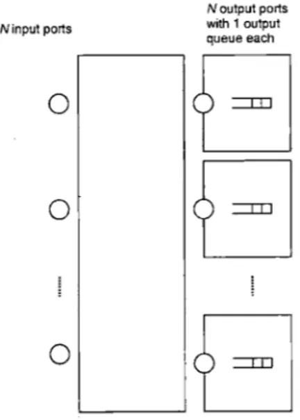
Output queuing is the most intuitive and ideal way of implementing the switching

operation. The idea behind output queuing is to make a packet available at its

destination as soon as it arrives to the switch. The switch is modeled as a black

box with input and output ports. We can assume without loss of generality that the

number of input ports and the number of output ports are equal to N.

N input ports

0

0

0

Figure 1-1: Output queued switch

In each time slot, packets arrive at the input ports and are destined to some

output ports. At most one packet can arrive to an input port during a single time

slot. At each output port, there is a FIFO queue that holds the packets destined to

that output, hence the name output queuing. When a packet destined to output

j

arrives to the switch, it is immediately made available at output

j

by storing it in

the appropriate output queue. At the end of the time slot, at most one packet can

be read from each output queue. This is very idealistic and no scheme can do better

since each packet is made available at its destination as soon as possible. However,

as we will see in the following section, this scheme is very problematic at high speed.

1.2

The Speedup Problem

It is possible that during a single time slot, the output queued switch will forward multiple packets to the same output queue. For instance, if during a time slot, packets at different inputs arrive to the switch and they all need to go to a particular output

j,

j.

single time slot. This implies that the memory speed of that queue has to be N times more than the line speed, which is limited to one packet per time slot. At a moderate line speed, this does not constitute a problem. However, output queuing becomes hard to scale at high speed. The line speed can be high enough to make the speedup factor

N impractical to achieve. Therefore, the use of output queuing becomes unfeasible at

high speed. We need a way to eliminate the undesired speedup. In order to overcome the speedup problem, we restrict the number of packets forwarded to an output port to one per time slot. As a result, an alternative architecture in which packets are queued at the input is suggested. The architecture, called Input Queuing, will make it possible to forward at most one packet to each output port and thus eliminates the need for a speedup.

1.3

Input Queuing

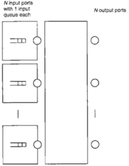
In input queuing, FIFO queues are used at the input ports instead of the output ports as depicted in the figure below.

A packet that cannot be forwarded to its output port during a time slot will be kept in its queue at the input. Note that no output queues are needed in this architecture since at most one packet will be forwarded to an output port during a single time slot. This packet will be consumed by the output port by the end of the time slot, and hence there will be no need to store any packets at the output. In order not to recreate the same speedup problem at the input side however, only one packet will be forwarded from an input port during a single time slot as well. Therefore, the

N input ports

with 1 input N output ports queue each

Figure 1-2: Input queued switch

set of packets that are forwarded during a particular time slot satisfies the condition that no two packets will share an input or an output. In other terms, among the forwarded packets, no two packets originate at the same input and no two packets are destined to the same output. We will see later how we can formally abstract this notion. Before doing so, let us examine a phenomenon that arises with input queuing known as Head Of Line blocking.

1.3.1

HOL Blocking

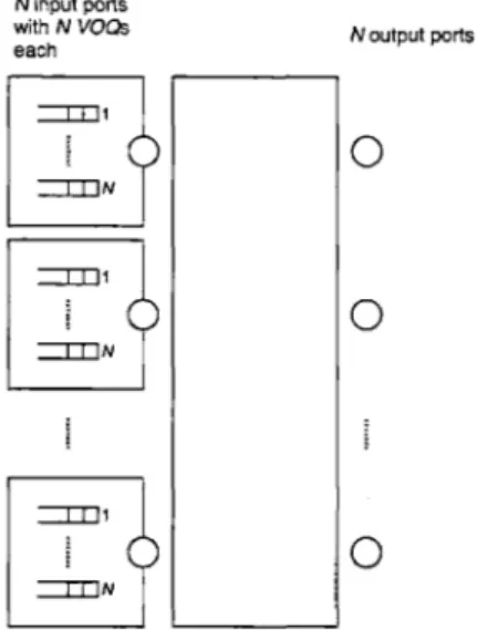
Head Of Line (HOL) blocking occurs when a packet at the head of the queue blocks all the packets behind it in the queue from being forwarded. This phenomenon can occur with input queuing when at a given time slot, two (or more) packets at different input ports need to be forwarded to the same output port, say output port j. Only one of these two packets can be forwarded; therefore, the one that will remain at the head of its queue will block other packets in the queue (which are possibly destined to outputs other than output j) from being forwarded. The HOL blocking phenomenon usually limits the throughput of the input queued switch [17]. One way to eliminate HOL blocking is by virtually dividing each input queue in to N queues, called Virtual Output Queues VOQs. A VOQ at an input will hold packets that are destined to one of the N outputs. Therefore, these VOQs can be indexed by both their input

and output ports. We denote by VOQg

the VOQ at input i holding packets destined

to output

j.

In this way, two packets that are destined to different output ports

cannot block each other since they will be stored virtually in two different queues.

The architecture is depicted below:

N input ports with N VOs each ITDN --- IN I IJN N output ports

0

0

0

Figure 1-3: Input queued switch with VOQs

In the next section, we provide a formal abstraction for the operation of the input

queued switch. We will see that the operation of the input queued switch can be

modeled as a computation of a matching (definition below) in every time slot.

1.3.2

Formal Abstraction

We address in this section the question of how to formally abstract the operation of

the input queued switch. We know that we can forward at most one packet from

an input port and at most one packet to an output port during a single time slot.

What is the theoretical framework that will give us this property? It is going to be

the notion of a matching. Intuitively speaking, the switch will match input ports to

output ports during each time slot. We start with few simple definitions:

Definition 1.1 (graph) A graph G

=

(V, E) consists of two sets V and E where V

is a set of nodes and E is a set of edges. Each edge in E connects two nodes in V.

which the set of nodes V = L U R is such that L and R are disjoint and every edge in E connects a node in L to a node in R.

We now define the matching.

Definition 1.3 (matching) A matching in a graph G = (V, E) is a set of edges in

E that are node disjoint.

Given the above definitions, we can now formally describe the operation of the input queued switch. In every time slot, the switch performs the following:

Formal Abstraction

let VOQij be the Jth queue at input i

construct a bipartite graph G = (L, R, E) as follows: an input port i becomes node i in L

an output port j becomes node j in R

a non-empty VOQij becomes edge (i, j) in E

compute a matching M in the bipartite graph G = (L, R, E)

Figure 1-4: Formal operation of the input queued switch

Since each edge represents a non-empty VOQ, the matching represents a set of packets (the HOL packet of each VOQ). Furthermore, since a matching is a set of edges that are node disjoint, the matching guarantees that these packets do not share any input or output ports, and hence they can be forwarded with no speedup.

1.4

Input-Output Queuing

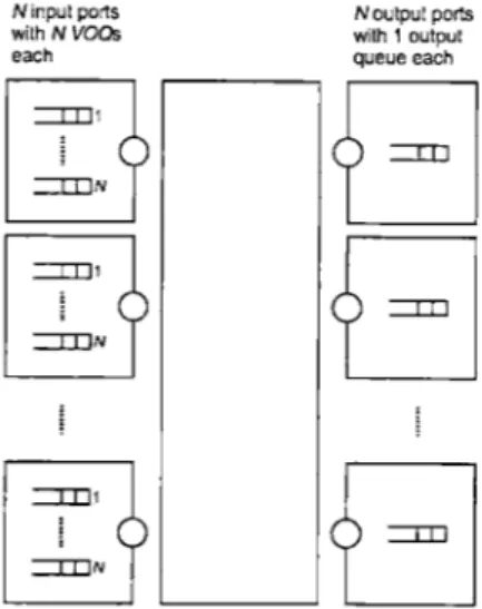
Although we developed our theoretical framework for an input queued switch based on the idea that the switch has no speedup, it is possible to consider an input queued switch with speedup. In fact, it has been shown that a limited speedup (independent of N) is useful for providing certain guarantees in an input queued switch [6], [7], [18].

However, as before, this requires the use of output queues at the output ports as well since more than one packet can be forwarded to an output port during a single time slot. We call such an architecture an input-output queued switch. Below we present

an input-output queued switch with VOQs.

N input ports Noutput ports

with N VO s with 1 output each queue each

-aN

-- 01

-N

ZoN

Figure 1-5: Input-Output queued switch with VOQs

Our theoretical framework based on matchings can still be used. However, an input-output queued switch with speedup will be able to compute matchings at a rate higher than one matching per time slot. For instance, with a speedup of 2, an input-output queued switch will compute two matchings per time slot. In general, the speedup needs not be necessarily an integer. We will model the input-output queued switch with continuous time as follows: With a speedup S> 1, the switch computes a matching every I time units, keeping in mind that S needs not be an integer. The line speed will be one packet per time unit and hence S is, as before, a speedup with respect to the line speed. Therefore, the switch will have successive matching phases where each matching phase takes I time units. When S = 1, i.e. a matching phase takes exactly one time unit, we get back our previous model of input queuing with no speedup. Note that in this case, no queues are necessarily required at the output.

To summarize what has been presented so far, we eliminated the speedup of N required with the idealistic output queuing using input queuing, by replacing the output queues with input queues instead. Moreover, we eliminated the phenomenon

known as HOL blocking by virtually splitting each input queue into N VOQs. We formally modeled the operation of the input queued switch as a computation of a matching in every time slot. Finally, we generalized our model to an input-output queued switch with a continuous time framework and a possible speedup S, where the switch computes a matching every I time units.

The question to ask now is why aren't we done with the problem of switching. The answer to this question is the following: what we did so far is reduce the problem of switching into a problem of computing a matching in a bipartite graph. A graph con-tains possibly many matchings and, therefore, we need to decide on which matching to choose. This decision problem is at the heart of performing the switching operation in input queued switches. As it will be seen in Chapter 2, if we are not careful on which matchings to choose, it is possible for some VOQs to become starved and grow indefinitely. Therefore, some algorithms have been suggested in order to compute the matchings (one every I units with a speedup S) without starving the VOQs (more formal definitions of this guarantee appear in Section 1.6). Before we look at some of these algorithms, we need to understand some aspects pertaining to the traffic of packets at the input. For this, we assume the existence of a traffic model.

1.5

Traffic Models

In this thesis, we will present three traffic models. A traffic model describes the arrival of packets to the switch as a function of time. A traffic model can be probabilistic or deterministic as it will be seen shortly. Before we proceed to the different traffic models, we need to define a quantity that tracks the number of packets arriving to the switch. Let Ai(t) be the number of packets arriving to the switch by time t that originate at input i and are destined to output j.

1.5.1

SLLN Traffic

This traffic is a probabilistic model that obeys the Strong Law of Large Numbers, hence its name SLLN. The Strong Law of Large Numbers says that if we have

indepen-dent and iindepen-dentically distributed (i.i.d.) random variables X, then Pr[lim-

Li

E[X]] = _{1, where E[X] is the expected value of the random variable X,. We say that}

L",iX"converges

n

packet arrivals are i.i.d. or not, we assume that lim. A 1(t) - A with probability

t

1, for some A5. In simpler terms, this means that it is possible to define a rate Aij for the flow of packets from input i to output

j.

SLLN:

*

,

1

"

XX

<(a

*"XX

a

S <1

The second and third conditions of the SLLN model constrain the sum of rates at every input and output port to be less than or equal to a, which we will call the

loading of the switch. Finally, we require that a < 1. The reason behind this last constraint is that the traffic cannot exceed the line speed at any port, which is limited to one packet per time unit. Another reason behind this constraint is that a switch with no speedup cannot access more than one packet per time unit at any port, and hence a switch with no speedup will be overloaded if a > 1. This constraint on the loading of the switch will be present in all the traffic models presented hereafter.

With the above probabilistic traffic model, it is possible to define a rate for the flow of packets from input port i to output port

j.

1.5.2

Weak Constant Burst Traffic

In some sense, the weak constant burst traffic is a stronger model than SLLN because it is deterministic. However, it does not define a rate for the flow of packets from

hence the use of the term weak in the burst characterization of this traffic model.

Weak Constant Burst

*

a(t

-t

B

* Vt

5

EkAkJ(t2)

tI) + B

e a < 1

The model simply says that for any time interval [t,7t 2], the maximum number of

packets that can arrive at an input i or destined to an output

j

where B is a constant independent of time and, as before, a is the loading of the switch.

Note that a is not necessarily the rate of packets at input i or output j. In fact, such a rate might not be defined. Thus, a is just an upper bound on the rate if it exists. Next we define a stronger traffic model that also satisfies this constant burst property.

1.5.3

Strong Constant Burst Traffic

The following model implies the previous model and hence is stronger (more con-strained).

Strong Constant Burst

* Vt1 t2, Aij(t 2) -

Ass(ti)

A(t

B

* Ek Aik a

* EkAkj< a

The model basically says that during any time interval [t1, t2], the number of

packets from input i to output

j

Note that both the weak constant burst and the strong constant burst models do not necessarily imply the SLLN model because limt,, !

7"

1.6

Guarantees

There are various service guarantees that one might want a switching algorithm to provide. In this thesis, we will address two basic guarantees. These are throughput and delay guarantees.

1.6.1

Throughput

Throughput basically means that as time evolves, the switch will be able to forward all the packets that arrive to the switch. There are many definitions of throughput and some definitions depend on the adopted traffic model. One possible definition of throughput under a probabilistic traffic model is for the expected length of each VOQ to be bounded. Therefore, if Xij(t) denotes the length of VOQjj at time t, we require that E[Xij(t)] _{; M < oo [21], [23], [24]. One can show that this implies that for any} E > 0, there exists a time to such that for every t > to, Pr[ ] _ c. We call this type of convergence, convergence in probability. Therefore, Xi1 _t(Q converges to 0 in

probability. Convergence in probability is weaker than convergence with probability 1 (see previous section). Other definitions of throughput require that under an SLLN traffic, himt", Dij(t) = _{with probability 1 [8], where Di}

1(t) = A 1(t) - Xii(t).

implies that lim=A D (t) Ai in probability. It is possible to show that if E[XJ (t)] is bounded, then lim = 0 with probability 1, which in turn implies that

limiteDi()=Aij with probability 1 if limt, , *,, =Aiwith probability I.

In this thesis, we will use two definitions of throughput. A weak definition and a strong definition.

Definition 1.4 (weak throughput) Let Xij(t) be the length of VOQj, at time t.

Then limte,0 x3(t) =0

The above definition can be also expressed as follows: for every e > 0, there exists a time to such that for any time t > to, XI(t) _t < - c.

Note that in the above definition, the throughput does not rely on the fact that lim> " (t) exists. Note also that the definition does not impose any strict bound on the size of the VOQs. Below we provide a stronger definition of throughput.

Definition 1.5 (strong throughput) Let Xij(t) be the length of VOQjj at time t. Then there exists a bound k such that Xij(t) < k for all t.

Obviously, strong throughput implies weak throughput.

It is useful to ensure that the queue size is bounded at any time since this will provide an insight to how large the queues need to be in practice. Most of the time however, this notion of strong throughput can be superseded by the delay guarantee described below. We will rely on the notion of weak throughput in Chapter 2 for proving some negative results on speedup, namely that some switching algorithms cannot achieve weak throughput without speedup.

If we have a throughput guarantee and the loading of the switch is a, we usually refer to this as a throughput. This notion is useful if we would like to observe the throughput guarantee as we change the loading of the switch. If there is a value a of the loading beyond which the switching algorithm cannot guarantee throughput, then we say that the algorithm guarantees a throughput.

1.6.2

Delay

Delay is a stronger guarantee than throughput and it basically means that a packet will remain in the switch for at most a bounded time.

Definition 1.6 (delay) Every packet remains in the switch for at most a bounded

time D.

Obviously, delay implies strong throughput. To see why this is true, define k =

[SD1 where S is the speedup of the switch. If the length of VOQjj exceeds k, then

at least one packet will remain in VOQjj for more than D time units since the switch can forward at most [SD] packets during an interval of time D from VOQ₂j, hence

violating the delay bound. Therefore, the length of VOQjj cannot exceed k.

1.7

Existing Switching Algorithms

Now that we have defined some traffic models and possible guarantees, we can enu-merate some of the existing switching algorithms. Recall that these will determine how to compute a matching every - time units with a speedup S. So we will first consider some properties of matchings in general.

Definition 1.7 (maximal) A matching M is maximal if there is no edge (i,

J)

such that M U (i, J) is a matching.

In simpler terms, a maximal matching is a matching such that no edge can be added to it without violating the property of a matching. Therefore, any edge outside the matching shares a node with at least one edge in the matching.

Definition 1.8 (maximum size) A matching M is a maximum size matching if

there is no other matching M' such that jM'| > |M|.

In simpler terms, a maximum size matching is a matching with the maximum possible number of edges. As a generalization to the maximum size matching we have the following definition.

Definition 1.9 (maximum weighted) In a weighted graph where edge (i, J) has weight wij, a matching M is a maximum weighted matching if there is no other

matching M' such that Z(ij)cM' Wij > E(ij)M i.

In simpler terms, a maximum weighted matching is a matching that maximizes the sum of weights of its edges.

The following sections describe some of the existing switching algorithms and the ways by which they compute the matchings.

1.7.1

Maximum Weighted Matching

This algorithm has been known for a while and is one of the first switching algorithms suggested in the literature. It is based on computing a maximum weighted matching as follows. In every matching phase, the weight of edge (i, j), w, is set according to some scheme. Then a maximum weighted matching based on these weights is com-puted. When wiy is the length of VOQjj (or the time the oldest packet of VOQj 1 has been waiting in VOQij) it has been shown that the expected length of any VOQ (or the expected wait for any packet) is bounded, with no speedup (S = 1) under an i.i.d. Bernoulli traffic in which a packet from input i to output

j

where M is the number of non-empty VOQs (i.e. edges in the bipartite graph, which could be O(N 2_{) making the required time O(N} 3_{)). This is the best known time}

re-quired to compute a maximum weighted matching in a bipartite graph [27]. This is not very practical at high speed. A variation on the definition of the weights can reduce the problem of computing a maximum weighted matching to computing a

maximum size matching [24]. This will have a time complexity of 0(v/M), which is the best known time required to compute a maximum size matching in a bipar-tite graph [27]. Unfortunately, O(N 2

-) time complexity is still not practical at high speed. Therefore, alternative switching algorithms have been suggested.

1.7.2

Priority Switching Algorithms

In order to overcome the complexity of the above switching algorithms, which are based on computing a maximum weighted matching, a family of algorithms that com-pute a matching based on a priority scheme emerged. Below is the general framework by which these algorithms compute their matchings.

Priority Switching Algorithm

start with an empty matching M = 0 prioritize all VOQs

repeat the following until M is maximal

choose a non-empty VOQij with a highest priority if M U (i, j) is a matching, then M = M U (ij) discard VOQij

Figure 1-6: Priority switching algorithms

Obviously, the time required to compute the priorities has to be efficient (for instance, it has to be o(N 3)); otherwise, the use of such an algorithm is not justified.

As an example, we can think of an algorithm that operates as follows: it computes a maximum weighted matching M as described in Section 1.7.1, and then assigns high priorities to all VOQij such that (i,

J)

outlined in Figure 1-6 based on these priorities. This is a priority switching algorithm that provides the same guarantees as the maximum weighted matching algorithm. However, the use of this algorithm is not justified because it requires O(N 3_{) time to} compute the priorities. Therefore, a requirement for the use of a priority switching algorithm is that the priority scheme itself is efficient to obtain.

Many priority schemes have been suggested. One algorithm called Central Queue [16] assigns higher priority to VOQs with larger length (the way the algorithm is presented here is slightly different than how it was originally presented in [16]). This

algorithm can be shown to guarantee strong throughput with no speedup when a < I if Aj (t) does not exceed Ajt by more than a constant for any time t. Moreover, if

Aij (t) is always within a constant from it, it was proved to provide a delay guarantee

with no speedup when a < 1. This algorithm, of course, requires the switch to be less than half loaded.

Another algorithm called Oldest Cell First [6] assigns higher priority to VOQs with older HOL packet, where the age of the packet is determined by the time it has been waiting in its VOQ. This was proved to provide a delay guarantee under a weak constant burst traffic with a speedup S > 2. It also provides strong throughput under a strong constant burst traffic with a speedup of 2.

Yet another algorithm called Lowest Occupancy Output Queue First LOOFA [18] assigns higher priority to a VOQj1 for which output queue

j

In Chapter 3, we are going to describe two priority switching algorithms that we propose. Both algorithms provide strong throughput with a speedup S = 2 and a delay guarantee with a speedup S > 2 under appropriate traffic models. The advantage of these two algorithms is that they require a considerably smaller amount of state information to compute the priorities than the previous priority switching algorithms.

Obviously, regardless of what the priority scheme is, the time complexity of a priority switching algorithm is Q(N 2). Although this is still considered impractical

at high speed, as discussed above these algorithms provide delay guarantees with appropriate traffic models and speedup. In Chapter 2, we will have a more general look at these algorithms and prove that the speedup requirement is inherent for these algorithms to provide even a weaker guarantee, like throughput, under a very restricted traffic model.

1.7.3

Iterative Switching Algorithms

So far, all the switching algorithms mentioned above require the need for a centralized global computation of matchings, which is the reason behind their high computational complexity. To overcome this requirement, a family of algorithms, called iterative, has been suggested. In these algorithms, the matching is computed in a distributed fashion where input and output ports interact independently in a simultaneous way. Such algorithms exploit some degree of parallelism in the switch that is acceptable, and in fact they were found to be very practical to implement in hardware.

As the name indicates, an algorithm belonging to this family works in multiple iterations within every matching phase, where in each iteration a partial matching is computed according to the following RGA (stands for Request, Grant, Accept) protocol. In each iteration, inputs and outputs interact independently in parallel: each unmatched input requests to be matched by sending requests to some outputs. Then each unmatched output grants at most one request. Finally, each unmatched input accepts at most one grant. If input i accepts a grant from output

j,

j

are matched to each other. It is obvious that the outcome of the RGA protocol is a matching since each output grants at most one request and each input accepts at most one grant.

Since multiple inputs can request the same output, and similarly, multiple outputs can grant the same input, the matching computed in one iteration is not necessarily maximal. For instance, an input receiving multiple grants has to accept only one of them and reject the others. This implies that some of the granting outputs could have granted other requests, but since there is no direct communication among the output ports themselves, this cannot be anticipated. Nevertheless, the size of the matching may grow with more iterations. As we will see in Chapter 4, these iterative switching algorithms do not provide high throughput (i.e. throughput for high values of ca) unless multiple iterations are allowed. The general framework of these algorithms is outlined in Figure 1-7 '.

'Some iterative switching algorithms allow for an input and an output to be unmatched in a future iteration in favor of another matching, based on priorities at the input and output ports.

Iterative Switching Algorithm

start with an empty matching M = 0

repeat for a number of iterations

R: unmatched input i Requests some outputs

G: unmatched output j Grants at most one request

A: unmatched input i Accepts at most one grant

if input i accepts a grant from output

j

M = M U (i,j)

Figure 1-7: Iterative switching algorithms

Iterative switching algorithms differ by how requests are prepared and how grants and accepts are issued. Examples of these algorithms are PIM (parallel iterative matching) [1], iSLIP [22], iPP (iterative ping-pong) [13], DRR (dual round robin) [20], and pDRR (prioritized dual round robin) [9]. In PIM, an unmatched input i sends requests for all outputs

j

iSLIP replaces randomness with the round robin order. As a result, each output

maintains a pointer to the inputs, and grants a request by moving the pointer in a round robin fashion until it hits a requesting input. The accepts are issued in a similar manner at the inputs. Other iterative algorithms (except for iPP) are variations on this idea. The time complexity of these algorithms is dominated by the complexity of one iteration, which basically consists of the RGA protocol. Depending on the algorithm, this could be 0(logN) or O(N), keeping in mind that ports operate in parallel. These algorithms provide a better alternative at high speed; however, they do no provide strong theoretical guarantees as we will see in Chapter 4.

Figure 1-7 does not reflect that possibility. Such algorithms are usually based on computing what is knows as stable marriage matchings [12] where input and output ports change their match repeatedly in successive iterations until the matching is stable and no more changes occur. Stable marriage matching algorithms require in general N2 iterations to stabilize. For an example, see [7] which presents an emulation of output queuing using an input queued switch with a speedup of 2.

1.8

Thesis Organization

The thesis is organized as follows. Chapter 2 will establish some lower bounds on the

speedup required for different classes of switching algorithms to guarantee throughput.

In Chapter 3, we propose two priority switching algorithms. The two algorithms

will provide strong throughput with a speedup S

=

2 and a delay guarantee with a

speedup S> 2 under appropriate traffic models. They offer the advantage of requiring

a smaller amount of state information than other priority switching algorithms. In

Chapter 4, we propose an iterative switching algorithm that provides high throughput

in practice with one iteration only. The algorithm will also provide, with only one

iteration, a delay guarantee with a speedup S5> 2 as well as strong throughput with

a speedup of 2. The property of requiring one iteration only makes it possible to

scale the switch at higher speeds since one matching phase will need to fit only one

iteration of the RGA protocol described above. Chapter 5 will investigate the use of

multiple input-output queued switches with no speedup in parallel in order to achieve

a delay guarantee while eliminating the speedup requirement imposed on the switch.

Chapter 6 continues with the idea of using parallel switches (not necessarily

input-output queued) and exploits a setting in which flows cannot be split across multiple

switches. Finally, we conclude the thesis in Chapter 7.

Chapter 2

Some Lower Bounds on Speedup

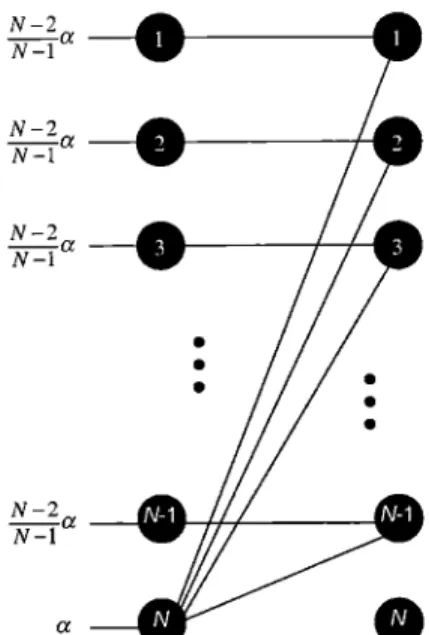
In this chapter, we establish some lower bounds on the speedup required to achieve throughput with different classes of switching algorithms. We will use the notion of weak throughput defined in Chapter 1. This will strengthen the results since an algorithm that cannot achieve weak throughput, cannot achieve strong throughput as well. We show a lower bound on the speedup for two fairly general classes of priority switching algorithms: input priority switching algorithms and output priority switching algorithms. These are to be defined later in the chapter, but for now, an input priority scheme prioritizes the VOQs based on the state of the VOQs while an output priority scheme prioritizes the VOQs based on the output queues. For output priority switching algorithms, we show that a speedup of 2 is required to achieve weak throughput. We also show that a switching algorithm based on computing a maximum size matching in every matching phase does not imply weak throughput unless S > 2. The bound of S > 2 is tight in both cases above based on a result in [8]. The results states that when S> 2, a switching algorithm that computes a maximal matching in every matching phase, achieves weak throughput with probability 1 under an SLLN traffic. Finally, we show that a speedup of is required for the class of input priority switching algorithms to achieve weak throughput.

Our model of a switch will be essentially the same general model of an input-output queued switch depicted in Figure 1-5. As before, the switch operates in matching phases, computing a matching in every phase. We will assume that the

switch computes a maximal matching in every phase. A switch with speedup S takes

1 time units to complete a matching phase before starting the next phase. Therefore,

if S > 1, output queues are also used at the output ports since packets will be forwarded to the output at a speed higher than the line speed. We review below some of the known results regarding the speedup of the switch.

Charny et al. proved in [63 that any maximal matching policy (i.e. any switching algorithm that computes a maximal matching in every matching phase) achieves a bounded delay on every packet in an input queued switch with a speedup S> 4 under a weak constant burst traffic. We will prove that the simple policy of computing any maximal matching does not imply weak throughput for a speedup S < 2. In fact, as mentioned earlier, we prove that even a maximum size matching policy does not imply weak throughput for S < 2.

Since switches with speedup are not desired due to their manufacturing cost and impracticality, it is very legitimate to look at what loading a a switch with no speedup (i.e. S = 1) can tolerate. The first work that addresses this issue appears in [16]. They provided a switching algorithm (called Central Queue algorithm) that computes a i-approximation of the maximum weighted matching, where they used the length of VOQjj as the weight for edge (i,

J)

In [6], the authors provide an algorithm called Oldest Cell First that guarantees a bounded delay on every packet with a speedup S > 2 under a weak constant burst traffic. The same algorithm can be proved to achieve strong throughput with a speedup of 2 under a strong constant burst traffic. This switching algorithm is a

priority switching algorithm and assigns higher priority to VOQs with older HOL packets. We will similarly prove that this algorithm cannot achieve weak throughput unless S

>

In another work [18], Krishna et al. provide an algorithm called Lowest Occupancy

Output Queue First LOOFA that guarantees a bounded delay on every packet with

a speedup of 2 and a strong constant burst traffic, and uses a more sophisticated priority scheme. This algorithm has also a work conservation property that we are not going to address here. The same lower bound of S> 1 applies for this algorithm as well in the sense that LOOFA does not imply weak throughput unless S>

2.1

Traffic Assumptions

We define a restricted model of traffic under which we are going to prove our lower bound results on S. Note that a more restricted traffic yields stronger results. Definition 2.1 An a-shaped traffic is a traffic that satisfies the following:

* VtI t2, Aij(t 2) - Aij(t 1) = j(t2 - t1) ± 0(1), where

A

"

Ek

ti)

*

,

t

± 0(1)

* Yk Aik _ a

e k Ak j a

a < I

The above conditions state that the rate of the flow from input i to output

j

The a-shaped traffic is the model under which we are going to prove the various lower bound results. As a consequence, the results will hold for all traffic models defined in Chapter 1, namely the SLLN traffic, the weak constant burst traffic, and the strong constant burst traffic.

2.2

Priority Scheme

In this section, we formally define a priority scheme. Recall from Chapter 1 that a priority scheme imposes an order on the VOQs by which they are considered for the matching. We first define an active VOQ to be a non-empty VOQ.

Definition 2.2 An active VOQ is a non-empty VOQ.

Definition 2.3 A priority scheme 7r defines for every matching phase m a partial

order relation lrm on the active VOQs.

We will use the notation VOQij rm.VOQkl to denote that VOQjj has higher priority than VOQkL during matching phase m. We will also use the notation

VOQiJgwmVOQkl to denote that VOQ2j does not have higher priority than VOQkl during matching phase m.

Note that since 7rm is a partial order relation, two VOQs might be unordered by 7r. In order for this to cleanly reflect the notion of equal priority, we define a well-behaved priority scheme as follows:

Definition 2.4 A well-behaved priority scheme ,r is a priority scheme such that for

every matching phase m, if VOQjj and VOQk, are unordered by T-,, and VOQkL and

VOQmn are unordered by 7r, then VOQjj and VOQ~n are unordered by rr.

The above condition on the priority scheme reflects the notion of equal priority. Hence if during a particular matching phase, VOQjj and VOQkL have equal priority, and VOQkI and VOQmn have equal priority, then VOQj 1 and VOQnn will have equal priority. This condition defines an equivalence relation on the VOQs which will help

us later to explicitly extend the partial order relation to a total order relation by which all VOQs are ordered.

In practice, a priority switching algorithm breaks ties among the VOQs with equal priorities. We will assume that ties are broken using the indices of the ports, and hence we assume the existence of a total order relation on the (i, j) pairs which is used for breaking ties. Adopting the assumption that breaking a tie among two

VOQs involves only the two VOQs in question and no other information, this is

the most general deterministic way of breaking ties, since anything else that is more sophisticated can be incorporated into the priority scheme itself. The definition below captures the idea.

Definition 2.5 Let wv be a well-behaved priority scheme and 0 be a total order relation

on the (i, j) pairs. We define the q extension of ir to be the priority scheme iro as fol-lows: For any matching phase m, if VOQij-<,VOQkI, then VOQijg< rVOQkl. For

any matching phase m, if VOQjj and VOQk, are unordered byirm, then VOQiJ-<0VOQkl

iff (Z', j) (k,31).

It can be shown that if ir is a well-behaved priority scheme, then 7r' is a priority scheme such that for every matching phase m, r orders all active VOQs. The fact that 7r is well-behaved means that 7rm induces the equal priority equivalence relation on the active VOQs. This in turn implies that we can extend 7r as described above without violating the property of an order relation. We omit the proof of this fact.

Note that our definition of a priority scheme is general enough to tolerate changing the definition of the partial order relation in every matching phase. Therefore, it is possible to prioritize the VOQs based on their lengths in one matching phase, and based on the age of their HOL packets in another.

Recall that a priority switching algorithm computes its matchings based on the given priority scheme (see Figure 1-6). We now define, for a given priority scheme 7r,

a matching that describes the outcome of a priority switching algorithm.

Definition 2.6 For a given priority scheme ,x, a matching computed in matching phase m is 7r-stable iff it satisfies the following condition: if an active VOQjj is not