OPERA TIONS RESEARCH
CENTER
Working Paper
MASSACHUSETTS INSTITUTE
OF TECHNOLOGY
A Comparison of Mixed-Integer Programming Models for
Non-Convex Piecewise Linear Cost Minimization Problems
by
Keely L. Croxton
Bernard Gendron
Thomas L. Magnanti
A Comparison of Mixed-Integer Programming Models for Non-Convex
Piecewise Linear Cost Minimization Problems
Keely L. Croxton
Fisher College of Business
The Ohio State University
Bernard Gendron
Departement d'informatique
et de recherche op6rationnelle
and
Centre de recherche sur les transports
Universit6 de Montreal
Thomas L. Magnanti
School of Engineering and Sloan School of Management
Massachusetts Institute of Technology
Abstract
We study a generic minimization problem with separable non-convex piecewise linear costs, showing
that the linear programming (LP) relaxation of three textbook mixed integer programming
formula-tions each approximates the cost function by its lower convex envelope. We also show a relaformula-tionship
between this result and classical Lagrangian duality theory.
Key words: piecewise-linear, integer programming, linear relaxation, Lagrangian relaxation.
Resum6
Nous considerons un probleme de minimisation gen6rique dans lequel l'objectif consiste d'une somme
separable de fonctions lineaires par morceaux non convexes. Nous montrons que les relaxations
lineaires de trois modeles classiques de programmation en nombres entiers sont equivalentes
puis-qu'elles fournissent comme approximation de l'objectif son enveloppe convexe inf6rieure. Nous
etablissons galement une relation entre ce rsultat et la th6orie de la dualite lagrangienne
clas-sique.
Mots-cls : lineaire par morceaux, progrmmation en nombres entiers, relaxation lin6aire, relaxation
lagrangienne.
1 Introduction
Optimization problems with piecewise linear costs arise in many application domains, including transportation, telecommunications, and production planning. In particular, many researchers have studied the minimum cost network flow problem with non-convex piecewise linear costs [1, 2, 4, 5, 6, 8]. Specific applications include the network loading problem [3, 13, 15, 19], the facility location problem with multiple capacity options [17, 18], and the merge-in-transit problem [7]. Each of these studies introduces integer variables to model the costs, though choice of the basic formulation varies and includes three textbook models, the so-called incremental, multiple choice and convex combination models. The objective of this note is to show that the linear programming (LP) relaxations of these mixed-integer programming (MIP) models are equivalent and that they all approximate the cost function by its lower convex envelope. To the best of our knowledge, although this result might appear to be intuitive, no one has formally established it. We also discuss the relationship between this result and classical Lagrangian duality theory.
We consider an arbitrary piecewise linear cost function like the one in Figure 1. The cost, g(x), is a function of a single variable, x, with the variable and fixed costs varying according to the value of x, which we call the load. The function need not be continuous; it can have positive or negative jumps, though we do assume that the function is lower semi-continuous, that is, g(x) liminf
x,-x g(x'). Without loss of generality, we also assume, through a simple translation of the costs if
necessary, that g(O) = 0.
The general problem is to minimize the separable sum of n piecewise linear functions, subject to linear constraints, which we write as:
minXEL g(x), (1)
n
with the objective function, g(x) = E gj(xj), defined over a bounded polyhedron L in R+ = {x E
j=1
IJnx > 0}. Since the formulations we consider model each function gj (xj) separately, for notational simplicity, we will drop the subscript j. We then let x denote a single variable and focus on a single piecewise linear function g(x). This simplification is justified by the fact that the lower convex
Cost
Load
Figure 1: A Piecewise Linear Cost Function
Cost
fs
,S
c
b(S-1) bs Load
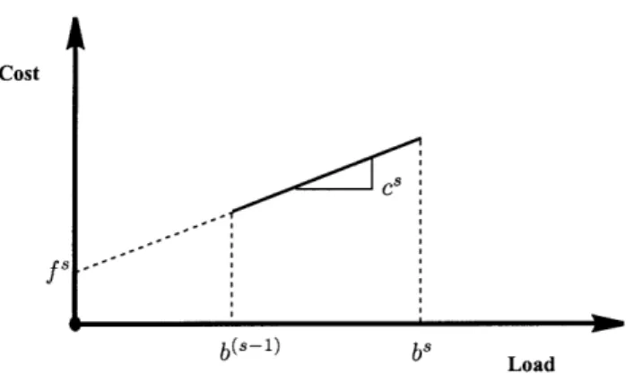
Figure 2: Notation for Each Segment
envelope of a separable sum of n functions (defined over a bounded polyhedron) equals the sum of the lower convex envelopes of these functions [11].
Each piecewise linear segment s E {1, 2,..., S} of the function g(x) has a variable cost, cS (the slope), a fixed cost, f (the cost-intercept), and upper and lower bounds, b-l and bS (the breakpoints), on the load corresponding to that segment. We assume b = 0. Figure 2 illustrates the notation.
Using this notation, in Section 2 we present three well-known valid MIP models for the problem. In Section 3, we show that the LP relaxations of the three formulations are equivalent and that they each approximate the cost function by its lower convex envelope. In Section 4, we discuss the relationship between this result and classical Lagrangian duality theory.
1
2
Three Models for Piecewise Linear Costs
To set notation, we introduce a formulation for each of the three models that we examine.
2.1
Incremental Model
Dantzig [9] and Vajda [21] both attribute the incremental model to a 1957 paper by Manne and Markowitz [20]. As reported in early textbooks, including those by Dantzig [10] in 1963 and Hadley [16] in 1964, the incremental model introduces a segment load variable, z, for each segment, defined as the load on the segment s. The final value of the variable, or load, x =
Es
zS, is the sum of theincremental quantities in each segment.
To be feasible using this variable definition, the value on segment s + 1 must be zero unless segment s is "full," that is, zs+ l > 0 only if zs = bs - bs - 1. To account for this requirement, the incremental model introduces binary variables, y, defined by the condition that yS = 1 if zs > 0, and y = 0 otherwise. Defining fs = (fS + csbs - ) - (fs-1 + cS-lbs-l) as the gap in the cost at the
breakpoint between segment s - I1 and segment s, we can express the piecewise linear optimization problem (1) as a MIP formulation by writing the objective function as g(x) =
E
8 cszs + fSyS, with the additional constraints:x= Ezs (2)
(b_ - bs-1)ys+1 < z < (bs - bs-l)ys, (3)
yS E
{0,
1}. (4)In this formulation, yS+l = 0 for the rightmost piecewise linear segment S of the cost function. We refer to this incremental system defined by (2)-(4) as I and its LP relaxation as LP(I).
2.2
Multiple Choice Model
The multiple choice model, as used by Balakrishnan and Graves [2], among others, employs an alternative definition of the segment variables. In this formulation, z equals the total load of x if that value lies in segment s. For this definition, if the total load equals x and x lies in segment s, z = H and z = 0 for all segments s s. As in the incremental formulation, yS = 1 if zs> 0, and
yS = 0 otherwise, but in this formulation at most one y will equal one. With this notation, the
multiple choice model has the objective function g(x) = E cSzS + fsys and the constraints:
x= Zs, (5)
bs-lys < z < bSy, (6)
E
y8
< 1,
(7)
ys e {0,1}. (8)
We refer to the multiple choice system defined by (5)-(8) as M and its LP relaxation as LP(M).
2.3 Convex Combination Model
The third formulation we examine is a modification of a formulation described in textbooks by Vajda [21] and Dantzig [10], and that appears as early as 1960 [9]. The original formulation was intended for continuous cost functions, so we modify it to handle arbitrary (lower semi-continuous) discontinuous functions. This formulation makes use of the fact that in a piecewise linear cost function, the cost of a load that lies in segment s is a convex combination of the cost of the two endpoints, bs-l and b, of segment s. By defining multipliers, /ts and As, as the weights on these two endpoints, we can write the objective function as g(x) = S,
IS(c
s b- + f) + AS(cSbSThe constraints are: X = 1(/zb5- + Vbb), (9) s + S = yS, (10)
E y
s< 1,
(11)
AS
>
0,y E
{0,1}.
(12)
In this formulation, the y variables have the same interpretation as in the multiple choice model. Constraint (11) assures that at most one of the y variables has value one. The constraints (10) assure that u + As = 1 for the segment corresponding to the positive yS variable, and that uS and AX are both zero for the other segments. Constraint (9) defines x to be the convex combination of the two endpoints defined by /u and A. We will denote the convex conbination system defined by (9)-(12) as C and its LP relaxation as LP(C).
3
Comparing the Three Models
Given that all three of the previous models are valid, and that researchers have used each of them in different application contexts, it is natural to ask if one is better than another. An important measure for assessing the quality of any MIP formulation is the strength of its LP relaxation. The following result demonstrates the equivalence of the LP relaxations of these three formulations.
Proposition 1 The LP relaxations of the incremental, multiple choice, and convex combination
formulations are equivalent, in the sense that any feasible solution of one LP relaxation corresponds to a feasible solution to the others with the same cost.
Proof: We establish this result by providing translations between feasible solutions of i) the
multiple choice and convex combination formulations; ii) the incremental and multiple choice for-mulations. We show that these translations give feasible solutions with the same cost.
Multiple Choice --* Convex Combination
Consider a feasible solution (x, y, z) to LP(M). Since b-'ys < z < bSys, for some value
of 0 < s < 1 zs = aSbs-lyS + (1 - as)bsys. Let ts =
cSyS
and As = (1 - a)yS. Then ,s + A s = y' and z = Sb-l + ASbs. Since x = E, z, x = Es(ZCb s - l + Asb S). Therefore, (x, y, t, A) is feasible for LP(C). The cost of this solution is Es/ S(cbs-1 + fs) + AS(csbs + fS) =Es cs(ps b
s
- l A s b s) + fS(/zS + AS) = E. cSzs + fsyS, which equals the cost of (x,y,z), the solution
to LP(M).
Convex Combination -- Multiple Choice
Consider a feasible solution (x, y, /, A) to LP(C). Define z = pSbs- 1 + ASbs. The conditions
bs -1 < bs and +A8 = yS imply that bS-lys < zs < by'. Therefore, (x, y, z) is feasible for LP(M). As shown previously, the cost of this solution is the same as the cost of (x, y, ut, A).
Incremental - Multiple Choice
Consider a feasible solution (x, y, z) to LP(I). Let w = zs+bS-lys - bsys+1 and vs= yS_ yS+l.
If we add bs-ly" - bSys+l to each of the terms in (3), these inequalities become b'-lvs < w < bSvs. The inequalities (3) imply that ys+l < ys, and thus vs> 0. In addition, Es v s= yl -yS+l = yl 1
(recall that yS+l = 0). Finally, E" w = Es zs+ b0y1- bSyS+1 = Es s z = x. Therefore, (x, v, w)
is a feasible solution to LP(M). The cost of this solution is
Es
cSwS + fSSv = ES cS(zS+ bS-lys-bsy+l
1) + fS(yS - yS+l) = Es cSzS +E
(fS + cb-)y s - ¥s(fS + cSbS)y s+ l = Es cSZS + [(fs +cSbs-l) - (fs-1 + cs-lbS-l)]y = E cSZS + fSyS, which equals the cost of (x, y, z).
Multiple Choice - Incremental
Consider a feasible solution (x,y,z) to LP(M). Let ws= zs + (bs- bs-1)(t,+l yt) - b"-lys and vs = ,t>s yt. These definitions imply that zs = wS + b-lv - bvs +l and ys = vs - v +l .
Also note that 0 < vs < 1. Through substitution, the inequalities (6) imply (bs - bS-l)vs +l < ws < (bS - bS-l)vs. In addition, Es w5 = Es zs= x. Therefore, (x, v, w) is a feasible solution to LP(I).
Moreover, using the same equations as in the translation from a solution of LP(I) to a solution of
LP(M), it is easy to show that the cost of (x, v, w) is the same as the cost of (x, y, z), the solution
We can further characterize the LP relaxation of these formulations with the following result:
Proposition 2 The LP relaxations of the incremental, multiple choice, and convex combination
formulations each approximate the cost function, g(x), with its lower convex envelope.
Proof: Since by Proposition 1 the three LP relaxations are equivalent, we need only show
that the LP relaxation of one of the formulations approximates the cost function with its lower convex envelope. We will use the convex combination formulation, showing that for any load 2, the objective value of the LP relaxation obtained by optimally choosing the other variables is given by the lower convex envelope of the cost function.
By relaxing the integrality restriction on the y variables, we can combine constraints (10) and (11) into Es(/ s + As) < 1 and we can eliminate the y variables. Therefore, a feasible solution is provided by any representation of x as a convex combination of the 2 S points, (bS, cSbs + fs), with
weight As, and (b - l, csbs-l + fs), with weight its. As we vary the value of , the cost minimizing convex combination is given by the lower convex envelope of these 2 S points. Because g(x) is piecewise linear, the lower convex envelope of these 2 S points is the same as the lower convex envelope of g(x).
In this discussion, we have developed the convex envelope property for the multiple choice and incremental models by establishing their equivalence to the convex combination model, for which the convex envelope result is readily apparent. Another approach would be to characterize the structure, especially for the extreme points, of their underlying LP feasible regions. This result might also be of interest in its own right.
Proposition 3 (Extreme Point Characterization)
(1) For any extreme point (, , ) of LP(M), the y variables assume a form with y^ = 0 for all s (when x = 0), or one y^ > O, or two Vs > 0 and their sum is one.
(2) For any extreme point (, , F) of LP(I), the y variables will be of the form s = 0 for all s (when = 0), or ys =
{,
if s<
and 0, if s > } for some indexg and constant 0 < _< 1, or{s
= {1, if s < tl, y, if tl < s < t2 and 0, if s > t2} for some indices tl, t2, and for some constant
0 < < 1.
Proof: See Appendix.
This result easily implies the convex envelope results for the multiple choice and incremental models. The alternatives when one gs > 0 or one s = y correspond to situations when the solution is either an endpoint of one of the piecewise segments of the objective function or is a combination of two endpoints, one being the origin.
4
Relationship to Lagrangian Duality
Assume that the nonempty bounded polyhedron L = x : Ax > b, 0 < x < u} representing the constraints of the piecewise linear optimization problem (1) is defined by an m x n matrix A, an m-dimensional vector b, and an n-dimensional vector u. Using this notation, we can rewrite problem
(1) as:
min g(x), (13)
Ax > b,
(14)0 <x < u. (15)
By associating a vector, y > 0, of m Lagrangian multipliers with the constraints (14) and letting gY(x) = g(x) -
yAx,
we can write the corresponding Lagrangian subproblem, LS(y), as follows:ZLS(y) = min g(x), (16)
subject to constraints (15). The corresponding Lagrangian dual, LD, is:
ZLD = max>o 'yb + ZLS().
8
To establish a relationship between Proposition 2 and classical Lagrangian duality theory, we will use the following theorem, due to Falk [11]:
Theorem 4 Let y* be an optimal solution to LD and x* an optimal solution to the corresponding
Lagrangian subproblem, LS(-y*). Then, x* minimizes the lower convex envelope of the cost function defined over the bounded polyhedron L.
To establish the desired relationship, we will show that ZLD equals the optimal value of the LP relaxation of any of the three formulations, say the multiple choice model (a similar development applies to the two other formulations).
First, note that we obtain gY(x) from g(x) by modifying only its slope through the introduction of the Lagrangian multipliers. Thus, gY(x) is a separable sum of n piecewise linear functions, which
n
we write as g7(x) = E g7(xj). Consequently, we can formulate the Lagrangian subproblem, LS(-y),
j=1
using the multiple choice model. Given the constraints of this model, we can assume that the bounding constraints (15) are redundant. The resulting problem decomposes into n subproblems, each of the form: min g(xj), subject to the constraints of the multiple choice model. If, for notational simplicity, we drop the subscript j, each of these n subproblems is defined by the objective function
ES
cS(y)zS + fyS and the constraints (5)-(8). In this expression, cS(y) is the slope of thesegment s modified by the introduction of the Lagrangian multipliers. Note that the total load variable, x, does not appear in the objective function. We can derive its value from the values of the segment load variables, z. Thus, we can remove constraint (5).
We could derive the same Lagrangian subproblem as follows: first, reformulate problem (13)-(15) using the multiple choice model; then, in the resulting MIP formulation, relax constraints (14) in a Lagrangian fashion. Clearly, the resulting Lagrangian dual is equivalent to LD, since the Lagrangean subproblems are identical. Classical Lagrangian duality theory in MIP [14] implies that the Lagrangian dual and the LP relaxation of the MIP model have equal optimal values if, for any cost function
>s
cS(y)zs + fSyS, the LP relaxation of the corresponding Lagrangian subproblemmultiple choice model if we can show that when we minimize some cost function
Es
cS(y)zs + fSySover the polyhedron P = {(y,z) : b-lys < zs bys, , ys __ 1, y > 0), the problem has an optimal solution with each yS E {0, 1}.
This property is easy to establish. Suppose we minimize some cost function Es cS(-y) z + fSyS
over the polyhedron P. If c(-y) > 0, then z = bS-lys in some optimal solution, while if c8(y) < 0, then z = bys in some optimal solution. Therefore, we can express each z in terms of the ys variables, and eliminate the z variables and the constraints bs-lys < z < by8. The resulting problem has a linear objective function and the single constraint Es yS < 1 in the nonnegative y variables. Since the problem has a single constraint, it has an optimal solution with at most one
y = 1 and all other y variables at value zero. Therefore, for some optimal solution the value of
each ys is 0 or 1.
This discussion shows how Lagrangian duality results imply the convex envelope property of the three classical models for optimization problems with non-convex piecewise linear costs. Conversely, it shows that the convex envelope property of the classical models presages the Lagrangian duality result and so further demonstrates the strong relationship between Lagrangian duality and linear programming.
5
Conclusion
We have shown that the LP relaxations of three textbook MIP models for non-convex piecewise linear minimization problems defined over bounded polyhedra are equivalent, each approximating the cost function with its lower convex envelope. We have also discussed the relationship between these results and classical Lagrangian duality theory.
The equivalence between the three LP relaxations and the fact that they all approximate the lower convex envelope of the cost function has several implications. First, it shows that from the perspective of linear programming relaxations, choosing among the three models is irrelevant. We might prefer one model to another for other reasons (for example, their use within specific
algorithms), but they all provide the same linear programming relaxations and bounds.
As an algorithmic implication, suppose we use a branch-and-bound algorithm to solve a non-convex piecewise linear cost minimization problem with a feasible region defined by a bounded polyhedron. There are two obvious relaxations for computing the lower bounds at the nodes of the enumeration tree: either the lower convex envelope or the LP relaxation of a MIP formulation of the problem. Falk and Soland [12] studied the first approach, but to the best of our knowledge, no one has ever recognized the fundamental relationship between their method and an LP-based branch-and-bound method: both compute the same lower bounds.
References
[1] Aghezzaf E.H., L.A. Wolsey (1994), Modeling Piecewise Linear Concave Costs in a Tree Parti-tioning Problem, Discrete Applied Mathematics 50, pp. 101-109.
[2] Balakrishnan, A., S. Graves (1989), A Composite Algorithm for a Concave-Cost Network Flow Problem, Networks 19, pp. 175-202.
[3] Bienstock, D., O. Giinliik (1996), Capacitated Network Design-Polyhedral Structure and Com-putation, INFORMS Journal on Computing 8, pp. 243-259.
[4] Chan, L., A. Muriel, D. Simchi-Levi (1997), Supply Chain Management: Integrating Inventory and Transportation, working paper, Northwestern University.
[5] Cominetti, R., F. Ortega (1997), A Branch & Bound Method for Minimum Concave Cost Network Flows Based on Sensitivity Analysis, working paper, Universidad de Chile.
[6] Croxton, K.L. (1999), Modeling and Solving Network Flow Problems with Piecewise Linear Costs, with Applications in Supply Chain Management, Ph.D. Thesis, Operations Research Center, Massachusetts Institute of Technology.
[7] Croxton, K.L., B. Gendron, T.L. Magnanti (2002), Models and Methods for Merge-in-Transit Operations, forthcoming Transportation Science.
[8] Croxton, K.L., B. Gendron, T.L. Magnanti (2002), Variable Disaggregation in Network Flow Problems with Piecewise Linear Costs, working paper, Operations Research Center, Mas-sachusetts Institute of Technology.
[9] Dantzig, G.B. (1960), On the Significance of Solving Linear Programming Problems with Some Integer Variables, Econometrica 28, pp. 30-44.
[10] Dantzig, G.B. (1963), Linear Programming and Extensions, Princeton University Press.
[11] Falk, J.E. (1969), Lagrange Multipliers and Nonconvex Programs, SIAM Journal on Control 7, pp. 534-545.
[12] Falk, J.E., Soland, R.M. (1969), An Algorithm for Separable Nonconvex Programming Prob-lems, Management Science 15, pp. 550-569.
[13] Gabrel, V., A. Knippel, M. Minoux (1999), Exact Solution of Multicommodity Network Op-timization Problems with General Step Cost Functions, Operations Research Letters 25, pp. 15-23.
[14] Geoffrion, A.M. (1974), Lagrangean Relaxation for Integer Programming, Mathematical
Pro-gramming Study 2, pp. 82-114.
[15] Giinlik, O. (1999), A Branch-and-Cut Algorithm for Capacitated Network Design Problems,
Mathematical Programming A86, pp. 17-39.
[16] Hadley, G. (1964), Non-Linear and Dynamic Programming, Addison-Wesley.
[17] Holmberg, K. (1994), Solving the Staircase Cost Facility Location Problem with Decomposition and Piecewise Linearization, European Journal of Operational Research 75, pp. 41-61.
[18] Holmberg, K., J. Ling (1997), A Lagrangean Heuristic for the Facility Location Problem with Staircase Costs, European Journal of Operational Research 97, pp. 63-74.
[19] Magnanti, T.L., P. Mirchandani, R. Vachani (1995), Modeling and Solving the Two-Facility Capacitated Network Loading Problem, Operations Research 43, pp. 142-157.
[20] Manne, A.S., H.M. Markowitz (1957), On the Solution of Discrete Programming Problems,
Econometrica, 25, pp. 84-110.
[21] Vajda, S. (1964), Mathematical Programming, Addison-Wesley.
Appendix
Proof of the Extreme Point Characterization:
(1) For any extreme point (,
,
2) of LP(M), the y variables assume a form with gS = 0 forall s (when 2-= 0), or one ys > O, or two gs > 0 and their sum is one.
We prove this result by showing that every extreme point of LP(M) is a convex combination of two endpoints of the piecewise linear segments, which follows directly from the following two facts, (a) and (b).
(a) Every extreme point of the polyhedron P={(y,z) : bS-lys < zs < bys,
As
ys < 1, ys > O} is anendpoint of one of the segments of the piecewise linear cost function. We established this result in our discussion of Lagrangian duality in Section 4 by showing that if we minimize some cost function
ES c'zS + fy 8 over the polyhedron P, the problem has a solution with at most one yS = 1 and all other y variables at value zero and with either z = b-lys or z = bys. Since any such point is an endpoint of a segment of g(x), and we have shown that such a solution is optimal for any choice of the cost coefficients, we conclude that any extreme point of P corresponds to an endpoint of a segment. Conversely, since we can choose the cost coefficients so that any endpoint of a segment is the unique minimizing solution, any endpoint of a segment corresponds to an extreme point of P.
(b) It is easy to see that if Q is any bounded polyhedron and we let wz = x be any linear equation, then every extreme point in the polyhedron Qx={z E Q : wz = x} is a convex combination of at most two extreme points of the polyhedron Q.
(2) For any extreme point (, y, 2) of LP(I), the y8 variables will be of the form S = 0 for all s (when = 0), or s = {, if s < and 0, if s > '} for some index and constant 0 < < 1, or
-S
0o < < 1.
We can establish this result using the same approach as with the multiple choice formulation. We first establish an analog of (a) for this formulation; letting As = bs - bs- l, we wish to show
that every extreme point of the polyhedron P={(y,z) ASy s+ l < zs < ASyS, 0 y 1} is an endpoint of one of the segments of the piecewise linear cost function. Suppose we minimize some cost function E cSzs+ fys over P. If cs > 0, then zs = Asys+ l in some optimal solution, while if
cs < 0 then z = ASys. Therefore, we can express each zs in terms of the yS variables and we are left with the following constraints: 0 < y < 1 and yS > yS+l. Any nonzero extreme point solution to this system is of the form y = 1, if s < and yS = 0, if s > , for some index