The MIT Faculty has made this article openly available.
Please share
how this access benefits you. Your story matters.
Citation
Arai, Tatsuya et al., "Comparison of cardiovascular parameter
estimation methods using swine data." Journal of Clinical
Monitoring and Computing 34, 2 (April 2020): 261–70 ©2019 Authors
As Published
https://dx.doi.org/10.1007/s10877-019-00322-y
Publisher
Springer Netherlands
Version
Author's final manuscript
Citable link
https://hdl.handle.net/1721.1/129354
Terms of Use
Creative Commons Attribution-Noncommercial-Share Alike
Author accepted manuscript
Cite this article as: Tatsuya Arai, Kichang Lee and Richard J. Cohen, Comparison of car-diovascular parameter estimation methods using swine data, Journal of Clinical Monitoring and Computinghttps://doi.org/10.1007/s10877-019-00322-y
This Author Accepted Manuscript is a PDF file of an unedited peer-reviewed manuscript that has been accepted for publication but has not been copyedited or corrected. The official version of record that is published in the journal is kept up to date and so may therefore differ from this version.
Terms of use and reuse: academic research for non-commercial purposes, see here for full terms.https://www.springer.com/aam-terms-v1
Author accepted manuscript
Comparison of Cardiovascular Parameter Estimation Methods Using Swine
Data
Tatsuya Arai1, and Kichang Lee2,3,Richard J. Cohen2,
Department of Aeronautics and Astronautics1 and Institute for Medical Engineering and Science2 Massachusetts Institute of Technology, Cambridge, MA 02139; the Cardiovascular Research Center3,
Massachusetts General Hospital, Boston, MA 02114
Running head: Cardiovascular Parameter Estimation
Corresponding Author:
Author accepted manuscript
Institute for Medical Engineering and Science
Massachusetts Institute of Technology
45 Carleton Street, Room E25-324
Cambridge, MA 02142
Voice: (617) 452-2718
Fax: (617) 253-3019
Author accepted manuscript
ABSTRACT 1
In this study, new and existing methods of estimating stroke volume, cardiac output and total
2
peripheral resistance from analysis of the arterial blood pressure waveform were tested over a wide range
3
of conditions. These pulse contour analysis methods (PCMs) were applied to data obtained in six swine
4
during infusion of volume, phenylephrine, dobutamine, isoproterenol, esmolol and nitroglycerine as well
5
as during progressive hemorrhage. Performance of PCMs were compared using true end-ejection
6
pressures as well as estimated end-ejection pressures.
7
There was considerable overlap in the accuracies of the PCMs when using true end-ejection
8
measures. However, for perhaps the most clinically relevant condition, where radial artery pressure is the
9
input, only Wesseling’s Corrected Impedance method and the Kouchoukos Correction method achieved
10
statistically superior results.
11
We introduced a method of estimating end-ejection by determining when the systolic pressure
12
dropped to a value equal to the sum of the end-diastolic pressure plus a fraction of the pulse pressure.
13
The most accurate estimation of end-ejection was obtained when that fraction was set to 60% for the
14
central arterial pressure and to 50% for the femoral and radial arterial pressures.
15
When the estimated end-ejection measures were used for the PCMs that depend on end-ejection
16
measures, when radial artery pressure was used as the input, only Wesseling’s Corrected Impedance
17
method and the modified Herd’s method achieved statistically superior results.
18
This study provides a systematic comparison of multiple PCMs’ ability to estimate stroke volume,
19
cardiac output, and total peripheral resistance and introduces a new method of estimating end-systole.
20 21
Key words — Arterial blood pressure; cardiac output; stroke volume; total peripheral resistance; pulse
22
contour method
Author accepted manuscript
Author accepted manuscript
INTRODUCTION 25
When managing patients undergoing high-risk surgeries (i.e., liver transplantation) or in the setting of 26
an intensive care unit (ICU), monitoring cardiovascular hemodynamic information such as stroke volume 27
(SV), cardiac output (CO), and/or total peripheral resistance (TPR) is critically important. In general, 28
these parameters respond much more quickly to stresses (i.e., hemorrhage) than does arterial blood 29
pressure (ABP) which is continuously controlled by multiple physiological feedback and control 30
mechanisms to maintain a homeostatic state [1]. Thus, the ability to monitor SV or CO may enable 31
clinical intervention at an earlier stage prior to the development of hypotension, shock, and/or organ 32
damage during surgeries or ICU stays. 33
The most commonly accepted method to estimate CO in clinical settings is pulmonary artery 34
thermodilution, which involves injecting a bolus of cold liquid through a central venous catheter into the 35
right atrium and measuring the temperature change in the pulmonary artery [2, 3]. In general, 36
thermodilution requires pulmonary artery catheterization, which is associated with cardiovascular risks 37
such as carotid artery puncture (when accessing the internal jugular vein), cardiac arrhythmia, bleeding, 38
embolism, clotting, and infection [4, 5]. Transpulmonary thermodilution has become an alternative to 39
pulmonary artery thermodilution [6]. However, previous research has shown several limitations 40
associated with its use [7, 8]. 41
Even though continuous thermodilution CO measurement could provide a continuous trend of CO 42
[9], thermodilution method cannot continuously measure SV on a beat-to-beat basis and has significant 43
limitations [10, 11]. Therefore, many studies have thus been devoted to developing non-invasive or 44
minimally invasive methods to continuously estimate cardiovascular parameters. These methods include 45
Doppler ultrasound, transesophageal echocardiography, and impedance plethysomography [12-15]. 46
However, due to various reasons, such as lack of accuracy, not providing continuous measurement, 47
technical difficulties, requiring a medical specialist, and/or economic reasons, these systems are not 48
popularly used and/or used only for calibration purposes in the clinical setting. 49
Author accepted manuscript
Since the arterial pulse is readily accessible, it has been commonly used to estimate the 50
cardiovascular parameters. Specifically, mathematical analysis of the continuous ABP, termed a pulse 51
contour method (PCM), has been extensively studied to estimate cardiovascular parameters [16-25]. 52
However, the clinical use of this method has also been limited due to its inaccuracy. 53
The present study aimed to evaluate new algorithms to estimate continuous cardiovascular 54
hemodynamic parameters. These methods were validated with measured CO using the true “gold 55
standard for aortic blood flow (ABF) measurement method” – Transonic’s ultrasonic flow probe placed 56
on the aortic arch of the study animal – and these predictive accuracies were compared with existing PCM 57
algorithms. In addition, for a fair comparison, a new algorithm for beat-to-beat identification of arterial 58
end-ejection blood pressure from peripheral arteries was incorporated into the cardiovascular 59
hemodynamic parameter estimation methods. 60
61
METHODS 62
The algorithms described in this section were evaluated using previously reported data (21). The 63
following is a brief summary of the protocol. Six Yorkshire swine (30–34kg) were studied. The 64
experimental protocol conformed to the Guide for the Care and Use of Laboratory Animals and was 65
approved by the MIT Committee on Animal Care. The animals were pre-anesthetized with intramuscular 66
telazol, xylazine, and atropine prior to endotracheal intubation. The swine were then maintained in a deep 67
plane of anesthesia using inhaled anesthetic isoflurane (0.5-4 %), a mixture of oxygen and ambient air. 68
Positive-pressure mechanical ventilation at a rate of 10-15 breathes/min, and a tidal volume of 10 ml/kg 69
was employed. 70
Central ABP (CAP) was measured from the thoracic aorta using a micromanometer-tipped catheter 71
(SPC 350, Millar Instruments, Houston, TX). Femoral ABP (FAP) and radial ABP (RAP) were measured 72
using external fluid-filled pressure transducer (TSD104A, Biopac Systems, Santa Barbara, CA). The 73
Author accepted manuscript
chest was opened with a midline sternotomy. ABF was recoded using an ultrasonic flow probe placed 74
around the aortic root for reference CO (T206 with A-series probes, Transonic Systems, Ithaca, NY). 75
ABF, ECG, and ABPs were interfaced to a microcomputer via an analog-to-digital conversion system 76
(MP150WSW, Biopac Systems, Santa Barbara, CA) at a sampling rate of 250 Hz and 16-bit resolution. 77
In each animal, a subset of the following interventions was performed over the course of 75 to 150 78
min to vary the cardiac output and other hemodynamic parameters: infusions of volume, phenylephrine, 79
dobutamine, isoproterenol, esmolol, nitroglycerine, and progressive hemorrhage. To achieve substantial 80
cardiac output changes in a short period (15-20 mins), several infusion rates were implemented followed 81
by brief recovery periods (about 5 min). Also, hemorrhage was performed until a substantial change in 82
cardiac output was observed. At the conclusion of the experiment, the animal was euthanized with the 83
injection of sodium pentobarbital. 84
85
Algorithms 86
Modified Herd’s Method: Pulse pressure (PP) is the difference between systolic blood pressure (SBP)
87
and diastolic blood pressure (DBP) and is regarded as a proportional measure of SV [16]. The algorithm 88
is based on the Windkessel model with impulse ejection of SV [28]. The drawback of using PP as a 89
proportional measure of SV is the inaccuracy introduced because of the finite duration of ejection and the 90
distortion/alteration of the ABP waveform as it propagates through the arterial tree. In general, as the 91
ABP waveform propagates through the tapered and bifurcated peripheral arterial branches, the SBP 92
increases and the ABP waveform width becomes narrower. 93
To overcome this latter issue, Herd et al. used mean arterial pressure (MAP) instead of SBP, since 94
MAP is less sensitive to this distortion [17]. However, when MAP is calculated by averaging the ABP 95
waveform, the value of MAP can be affected by the duration of the diastolic interval, resulting in an SV 96
estimation error. For example, a longer diastolic interval would result in a smaller SV estimate – even 97
Author accepted manuscript
though diastole follows the completion of ejection, and thus the length of diastole cannot affect the value 98
of the preceding SV. To overcome this limitation, we used mean pressure during ejection instead of mean 99
pressure averaged over the entire beat: 100
(Equation 1)
101
= arterial compliance, = arterial blood pressure waveform, and = ejection period. DBP is
102
the end-diastolic blood pressure of the preceding beat. 103
CO was estimated from time-averaging the SV values and TPR was calculated using the following 104
equation (Ohm’s law): 105
TPR CO
MAP (Equation 2)
106
CO and TPR estimates in the following methods were obtained in the same manner. 107
Auto-Regressive with Exogenous input (ARX) Model: We recently introduced a novel algorithm to 108
continuously estimate beat-to-beat ABF waveforms by analysis of the ABP signal. SV can be yielded by 109
the beat-to-beat integral of the ABF waveform, and CO can be calculated by the time average of ABF 110
over number of beats in a unit time. 111
In this section, the ABF estimation method will be briefly summarized (see Ref 26 for more details). 112
The mathematical model of the system can be described as an ARX input model that relates the ABP 113
values, , to the ABF values, : 114
(Equation 3)
115
where, are the autoregressive coefficients, is the parameter length, α is the weighting coefficient 116
for the exogenous input , and is noise. 117
Author accepted manuscript
Because the input ABF is approximately zero during diastole, the autoregressive coefficients can 118
be obtained by using a least-squares method to solve Equation 3: 119
(Equation 4)
120
where, designates a sample point during diastole. 121
The coefficients was obtained by solving the matrix equation using Matlab (Mathworks, Natick, 122
MA). A 17-beat moving window size was empirically found to be optimal with our algorithm for 123
estimating the coefficients and was therefore adopted. The autoregressive coefficient length was 124
chosen to minimize 125
The exogenous input weighting coefficient (α) was obtained by taking the average of both sides of 126
Equation 4: 127
(Equation 5)
128
where, MAP/CO can be obtained from Ohm’s law (Equation 2). 129
TPR is related to the and the characteristic time constant of the system (τ): 130
(Equation 6)
131
where, τ can be obtained by analyzing the terminal exponential decay curve of the impulse response of 132
the system : 133
(Equation 7)
134
Equations 5 and 6 can be combined to compute α: 135
(Equation 8)
136
Thus, instantaneous ABF can be expressed as: 137
Author accepted manuscript
(Equation 9)
138
The integral of was calculated on a beat-to-beat basis to obtain proportional SV estimates, and 139
the time average of over six minutes was calculated to obtain a proportional estimate of the CO 140
(proportionality constant being ). Thus, the algorithm presented here provides a comprehensive set of 141
proportional cardiovascular parameters (ABF, SV, CO, and TPR) based on an analysis of ABP 142
waveforms. 143
The calculated CO, SV, and TPR using these two methods were compared with those using the 144
previously reported methods. 145
Existing Pulse Contour Methods: Table 1 summarizes the existing cardiovascular parameter estimation
146
methods that were reported to be competitive in previous comparison studies [23, 27]. 147
Earlier works assumed that the arterial trees are represented by a two-parameter Windkessel model 148
accounting for the total compliance of the large arteries [arterial compliance ( )] and the TPR of small 149
arteries. During the diastolic period, the time constant (τ) is equal to the product of TPR and and the 150
proportional CO can be estimated using the time-averaged ABP and time constant [30]. Mukkamala et al. 151
calculated the time constant of the Windkessel model using an autoregressive moving average analysis 152
using arterial pressure and PP inputs to estimate the terminal projected exponential pressure decay during 153
diastole [21]. 154
Erlanger and Hooker described a relationship between SV and the PP suggesting that SV is 155
proportional to the PP [16]. Meanwhile, Herd et al. used MAP instead of SBP recorded in the ascending 156
aorta in the PP method to estimate robust SV [17]. When intra-aortic pressure is being measured 157
continuously, it is a relatively simple matter to subtract DBP from MAP and to multiply by the heart rate 158
(HR) to estimate CO. 159
Author accepted manuscript
Liljestrand-Zander reported that varied throughout the cardiac cycle and was dependent on ABP. 160
They used the inversely proportional relationship between and ABP to correct the non-linearity [20]. 161
Researchers also reported that SV is proportional to the area under the systolic region of the ABP 162
waveform [18, 19, 24, 25]. Kouchoukos et al. [19] and Wesseling et al. [25] proposed an empirical and 163
simple correction factor to the systolic area method to account for some source of error in ABP 164
fluctuations during the systolic period. Sun et al. [23] estimated SV using the root-mean-square of the 165
ABP waveform, which was claimed as one component of the LiDCOplus PulseCO method (LiDCO Ltd., 166
London, England). 167
The aforementioned methods use information regarding end-ejection. Traditionally, researchers have 168
used the dicrotic notch as an indicator of end-ejection. However, identifying the dicrotic notch can be 169
challenging since the dicrotic notch is often not detectable, particularly in the peripheral ABP signal. For 170
this reason, we estimated the end-systolic pressure values using the partial PP model. 171
Partial Pulse Pressure Model: An end-diastole always comes after a systolic peak. At end-ejection, the
172
pressure value is less than peak SBP. One can estimate the end-ejection pressure to correspond to the 173
ABP at the point in time when ABP falls to a value given by the following equation: 174
(Equation 10)
175
where, , , and are pressure values at end-ejection, end-diastole (previous beat), and peak
176
systole, respectively. 177
As examples, end-ejections identified by the 50% PP and 90% PP are shown in Figure 1. The time 178
stamp of can be regarded as the time of an estimated end-ejection. To determine the accuracy of the 179
PP model, we compared duration of diastole as estimated from the difference between the end-ejection 180
time determined by the partial PP Model and the onset of ejection as determined from the ABP signal 181
with the “true” duration of diastole as measured from the ABF signal. It was necessary to measure 182
Author accepted manuscript
duration of diastole because both end-ejection and onset of ejection time estimates in FAP and RAP are 183
delayed with respect to the true times of end-ejection and onset of ejection in the ABF signal measured in 184
the central aorta. We then determined the optimal value of the fraction f for each of the CAP, FAP and 185
RAP signals. The partial PP end-ejection identification method was then applied to the PCMs for 186
estimating SV, CO, and TPR. 187
The values of SV, CO, or TPR determined using the various algorithms are estimated to within a 188
proportionality constant (determined by ). Therefore, the comparison of estimated to measured values 189
of SV, CO, or TPR was achieved in each animal by adjusting the mean of each estimated parameter to 190
match the mean of the measured value. 191
For all methods, end-diastolic measures were computed from the preceding cardiac cycle. The 192
estimation errors are defined as root normalized mean squared error (RNMSE): 193
(Equation 11)
194
where, and are the measured and estimated values (i.e., SV, CO, and TPR), respectively, is
195
the number of data points, and is the number of free parameters. 196
RNMSEs of SV, CO, and TPR of each method with the true end-ejection pressure information were 197
compared with the other methods using analysis of variance (ANOVA). In addition, RNMSEs of SV, 198
CO, and TPR of each method with estimated end-ejection pressure using the partial PP model were 199
compared with the other six methods using ANOVA. If a significant difference was observed, simple 200
effects analysis with Duncan test was used to examine pair-wise differences (SAS 9.4). Statistical 201
significance was accepted at P<0.05. 202
RESULTS 203
Author accepted manuscript
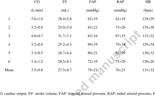
Interventions resulted in a wide range of changes of CO (1.3 – 5.8 L/min), MAP (27 – 127 mmHg), 204
and HR (91 – 204 bpm). Table 2 summarizes the physiological ranges of the data sets. Over 68,000 205
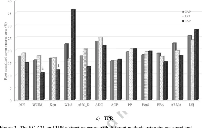
beats were processed and analyzed for ABF and hemodynamic parameters. Figure 2 shows the SV, CO, 206
and TPR estimation errors with different methods. While there was considerable overlap in the 207
accuracies of the PCM estimates, for perhaps the most clinically relevant estimations, which use RAP as 208
the input, only the Wesseling’s Corrected Impedance and the Kouchoukos Correction methods achieved 209
statistically superior results for all three of the estimated hemodynamic parameters. 210
Using the partial PP model, the end-ejection identification errors were minimum when the fraction f 211
in Eq. 10 was set to 60% for CAP, 50% for FAP, and 50% for RAP - as shown in Table 3. Thus, the most 212
accurate estimation of end-ejection was obtained when end-ejection was estimated to occur when systolic 213
pressure dropped to a value equal to the end-diastolic pressure plus 60% (50%) of the PP for the CAP (for 214
the FAP and RAP). Here the diastolic pressure and PP were referenced to the previous beat end-215
diastolic pressure. 216
In Figure 3, we show the RNSME results when using the estimated end-ejection time and pressures 217
for methods that depend on the end-ejection measures. The above optimal values of f were used here. 218
For the most clinically relevant condition where RAP is the input, only Wesseling’s Corrected Impedance 219
method and the modified Herd’s method achieved statistically superior results for all three of the 220
estimated hemodynamic parameters. In particular, Wesseling’s Corrected Impedance method provided 221
the lowest RNSMEs of 15.7% (SV), 12.3% (CO) and 12.9% (TPR). 222
223
DISCUSSION 224
In this paper, new algorithms were tested to estimate cardiovascular hemodynamic information. An 225
algorithm using the ARX model to continuously estimate ABF by the analysis of peripheral ABP 226
waveform was used to calculate CO, SV, and TPR. In addition, the modified Herd’s method was tested 227
Author accepted manuscript
and systemically compared with the existing hemodynamic parameter estimation methods using the same 228
ABP dataset. We also tested existing PCM algorithms and evaluated the impact of estimating end-229
ejection time and pressure on the performance of the PCM algorithms. 230
There was considerable overlap in the accuracies of the PCM estimates when using true end-ejection 231
pressures. However, for perhaps the most clinically relevant estimations, which use radial artery pressure 232
as the input, only the Wesseling’s Corrected Impedance and the Kouchoukos Correction methods 233
achieved statistically superior results for all three of the estimated hemodynamic parameters. 234
All the methods incorporate their own assumptions in cardiovascular physiology. Cardiovascular 235
hemodynamic parameter estimation methods need to work under a wide set of physiological conditions in 236
clinical and research settings. The parameters of Wesseling’s Corrected Impedance method [25] were 237
empirically obtained from a human study. In this method, the systolic area under the ABP curve above 238
DBP was scaled using a scaling factor that is a function of HR and MAP. Although the scaling factor 239
formula was obtained from healthy male subjects in their twenties, the method achieved low errors when 240
applied to the swine data sets, indicating that the human and swine cardiovascular system may be similar 241
in terms of applicability of the model. The Kouchoukos Correction method [19] includes a simple 242
correction factor (TS/TD) to model run-off blood flow during systole. Although the correction factors are
243
in both cases empirical, the Wesseling’s and Kouchoukos’s methods achieved lower errors than several 244
theoretical model-based methods. 245
Liljestrand-Zander’s method [20] unexpectedly generated high errors with the swine data, although it 246
has been reported to have the best agreement with the thermodilution CO in ICU patient data sets [23]. 247
This could be attributed to the nature of the ICU data sets. Because clinicians attempt to maintain the 248
patient’s ABP and CO, there is less variation in these signals obtained from patients than those obtained 249
during animal experiments in which these signals can be varied more widely using a variety of 250
interventions. Thus, methods that tend to provide stable estimates may appear to perform better with 251
Author accepted manuscript
patient data where the majority of the input parameters are stable. However, the utility of a method to 252
measure CO and other cardiac hemodynamic parameters is to identify those rare occasions when these 253
parameters deviate substantially from their normal values. The data analysis employed in this study was 254
designed to weigh the tail values specifically to test this aspect. 255
For the hemodynamic parameter estimation, end-systole (onset of diastole) needs to be determined for 256
each beat. In practical settings, a standard method to detect the end-systole (onset of diastole) is the use 257
of the dicrotic notch in ABP waveforms. However, the dicrotic notch does not always exist in the ABP 258
waveform. Therefore, we evaluated the performance of a model to estimate end-ejection (Eq. 10). 259
The most accurate estimation of end-ejection was obtained when end-ejection was estimated to occur 260
when systolic pressure dropped to a value equal to the end-diastolic pressure plus 60% (50%) of the PP 261
for the CAP (for the FAP and RAP). Here the end-diastolic pressure and PP are referenced to the 262
previous beat end-diastolic pressure. 263
In Figure 3, we show the RNSME results when using the estimated end-ejection pressures for 264
methods that depend on the end-ejection pressure. Here, for the most clinically relevant condition when 265
radial artery pressure is the input, only Wesseling’s Corrected Impedance method and the modified 266
Herd’s method achieved statistically superior results for all three of the estimated hemodynamic 267
parameters. In particular, Wesseling’s Corrected Impedance method provided the lowest RNSMEs. 268
The ARX algorithm utilizes the notion that the input to the arterial system is zero during diastole. In 269
the ABF estimation routine, 17 diastolic ABP waveforms were used to obtain the autoregressive (AR) 270
parameter and the AR parameters were integrated into the ARX model and applied to the entire ABP 271
waveform to obtain the ABF waveform. The AR parameters were also used to obtain the characteristic 272
time constant as well as the scaling factor to properly scale the estimated ABF. The 17-beat moving 273
window size was empirically chosen. If the window is too short, one cannot excite enough modes to 274
identify the system. On the other hand, if the window is too long, one cannot assume time-invariance of 275
Author accepted manuscript
the pertinent cardiovascular system. This method provides not only proportional SV, CO, and TPR, but 276
also instantaneous ABF waveforms without training data sets or demographic hemodynamic parameters - 277
arguably one of the most comprehensive estimation algorithms to our knowledge. 278
The classical Windkessel model assumes exponential decay during diastole and this model can be 279
described as a low-order AR model. The present ARX algorithm, on the other hand, obtains higher-order 280
AR parameter from diastolic ABP waveforms. The advantage of the present ARX algorithm is that it 281
appears to take into account possible distortion in the diastolic ABP waveforms in that the filter created 282
by the algorithm can reliably reconstruct the systolic ABF waveform. The distortion property may vary 283
from artery to artery, as well as from subject to subject. The algorithm could obtain individual parameters 284
unique to each arterial line of each subject on a beat-to-beat basis. 285
Further development of accurate end-systole identification methods (e.g., perhaps incorporating heart 286
sounds) might lead to more robust SV, CO, and TPR estimation using the new methods. Future work is 287
needed to apply and validate the algorithm with abnormal beats, such as premature beats and in heart 288
failure models. The methods could also be applied to optimizing SV when programming atrioventricular 289
time delay for conventional pacemakers and timing parameters for biventricular pacing. 290
One limitation of the current work is that the animal data involved using healthy pigs (~35 kg) with 291
normal hearts. Further studies would be necessary to apply the methods described here under a variety of 292
pathological clinical conditions (e.g. heart failure). The methods described here also need to be evaluated 293
using human data under various clinical conditions and populations. 294
295
CONCLUSION 296
Author accepted manuscript
This paper tested new algorithms to estimate hemodynamic parameters (SV, CO, and TPR) by 297
analysis of the ABP signal. Additionally, a new algorithm to identify end-ejection was implemented in 298
conventional and the new hemodynamic parameter estimation algorithms. 299
There was considerable overlap in the accuracies of the PCM estimates when using true end-ejection 300
pressures. However, for perhaps the most clinically relevant estimations, which use radial artery pressure 301
as the input, only the Wesseling’s Corrected Impedance and the Kouchoukos Correction methods 302
achieved statistically superior results for all three of the estimated hemodynamic parameters. 303
The Wesseling’s Corrected Impedance method and the modified Herd’s method performed best 304
among methods that depended on end-ejection time or pressure when estimated, rather than true, values 305
of end-ejection measures were used. In particular, the Wesseling’s Corrected Impedance method 306
provided the lowest errors. 307
Author accepted manuscript
Compliance with ethical standards 309
310
Conflict of Interest Richard Cohen is a co-inventor on two patents in the area of hemodynamic 311
parameter estimation assigned to the Massachusetts Institute of Technology (MIT) which have been 312
licensed to Retia Medical, LLC. Dr. Cohen is not otherwise involved with the company. The other 313
authors declare no conflicts. 314
315
Ethical approval All procedures performed in studies involving animals were in accordance with the 316
ethical standards of the institution. 317
318 319 320
Author accepted manuscript
REFERENCES 321
[1] H. Barcroft, O.G. Edholm, J. McMichael, and E.P. Sharpey-Schafer, "Posthaemorrhagic fainting. 322
Study by cardiac output and forearm flow," Lancet, vol. 1, pp. 489-491, 1944. 323
[2] W. Ganz, R. Donoso, H.S. Marcus, J.S. Forrester, and H.J. Swan, "A new technique for 324
measurement of cardiac output by thermodilution in man," Am J Cardiol, vol. 27, pp. 392-6, 1971. 325
[3] W. Ganz and H.J. Swan, "Measurement of blood flow by thermodilution," Am J Cardiol, vol. 29, 326
pp. 241-6, 1972. 327
[4] G.R. Manecke, Jr., J.C. Brown, A.A. Landau, D.P. Kapelanski, C.M. St Laurent, and W.R. Auger, 328
"An unusual case of pulmonary artery catheter malfunction," Anesth Analg, vol. 95, pp. 302-4, 329
2002. 330
[5] J.S. Vender and H.C. Gilbert, “Monitoring the anesthetized patient,” 3 ed. Philadelphia: Lippincott-331
Raven Publishers, 1997. 332
[6] X. Monnet and J.L. Teboul, “Transpulmonary thermodilution: advantages and limits,” Crit Care, 333
vol. 21, pp. 147, 2017. 334
[7] L. Huter, K.R. Schwarzkopf, N.P. Schubert, and T. Schreiber, “The level of cardiac output affects 335
the relationship and agreement between pulmonary artery and transpulmonary aortic thermodilution 336
measurements in an animal model,” J Cardiotheorac Vasc Anesth, vol. 21, pp. 659-63, 2007. 337
[8] K. Staier, M. Wilhelm, C. Wiesenack, M. Thoma, and C. Keyl, “Pulmonary artery vs. 338
transpulmonary thermodilution for the assessment of cardiac output in mitral regurgitation: a 339
prospective observational study,” Eur J Anaesthesiol, vol. 29, pp. 431-7, 2012. 340
[9] F.G. Mihm, A. Gettinger, C.W. Hanson, 3rd, H.C. Gilbert, E.P. Stover, J.S. Vender, B. Beerle, and 341
G. Haddow, "A multicenter evaluation of a new continuous cardiac output pulmonary artery 342
catheter system," Crit Care Med, vol. 26, pp. 1346-50, 1998. 343
Author accepted manuscript
[10] M. Botero, D. Kirby, E.B. Lobato, E.D. Staples, and N. Gravenstein, "Measurement of cardiac 344
output before and after cardiopulmonary bypass: Comparison among aortic transit-time ultrasound, 345
thermodilution, and noninvasive partial CO2 rebreathing," J Cardiothorac Vasc Anesth, vol. 18, pp. 346
563-72, 2004. 347
[11] W.H. Fares, S.K. Blanchard, G.A. Stouffer, P.P. Chang, W.D. Rosamond, H.J. Ford, and R.M. Aris, 348
"Thermodilution and Fick cardiac outputs differ: impact on pulmonary hypertension evaluation," 349
Can Respir J, vol. 19, pp. 261-6, 2012. 350
[12] M.E. Blohm, D. Obrecht, J. Hartwich, G.C. Mueller, J.F. Kersten, J. Weil, and D. Singer, 351
"Impedance cardiography (electrical velocimetry) and transthoracic echocardiography for non-352
invasive cardiac output monitoring in pediatric intensive care patients: a prospective single-center 353
observational study," Crit Care, vol. 18, pp. 603, 2014. 354
[13] S. Schubert, T. Schmitz, M. Weiss, N. Nagdyman, M. Huebler, V. Alexi-Meskishvili, F. Berger, 355
and B. Stiller, "Continuous, non-invasive techniques to determine cardiac output in children after 356
cardiac surgery: evaluation of transesophageal Doppler and electric velocimetry," J Clin Monit 357
Comput, vol. 22, pp. 299-307, 2008. 358
[14] S. Scolletta, F. Franchi, S. Romagnoli, R. Carla, A. Donati, L.P. Fabbri, F. Forfori, J.M. Alonso-359
Inigo, S. Laviola, V. Mangani, G. Maj, G. Martinelli, L. Mirabella, A. Morelli, P. Persona, D. 360
Payen, and PulseCOval Group, "Comparison Between Doppler-Echocardiography and Uncalibrated 361
Pulse Contour Method for Cardiac Output Measurement: A Multicenter Observational Study," Crit 362
Care Med, vol. 44, pp. 1370-9, 2016. 363
[15] R.P. Patterson, "Fundamentals of impedance cardiography," IEEE Eng Med Biol Mag, vol. 8, pp. 364
35-8, 1989. 365
Author accepted manuscript
[16] J. Erlanger and D.R. Hooker, "An experimental study of blood-pressure and of pulse-pressure in
366
man," Johns Hopkins Hosp Rep, vol. 12, pp. 145-378, 1904.
367
[17] J.A. Herd, N.R. Leclair, and W. Simon, "Arterial pressure pulse contours during hemorrhage in 368
anesthetized dogs," J Appl Physiol, vol. 21, pp. 1864-8, 1966. 369
[18] W.B. Jones, L.L. Hefner, W.H. Bancroft, Jr., and W. Klip, "Velocity of blood flow and stroke 370
volume obtained from the pressure pulse," J Clin Invest, vol. 38, pp. 2087-90, 1959. 371
[19] N.T. Kouchoukos, L.C. Sheppard, and D.A. McDonald, "Estimation of stroke volume in the dog by 372
a pulse contour method," Circ Res, vol. 26, pp. 611-23, 1970. 373
[20] G. Liljestrand and E. Zander, "Vergleichende Bestimmung des Minutenvolumens des Herzens beim 374
Menschen mittels der Stickoxydulmethode und durch Blutdruckmessung," Zeitschrift fur die 375
gesamte experimentelle Medizin, vol. 59, pp. 105-122, 1928. 376
[21] R. Mukkamala, A.T. Reisner, H.M. Hojman, R.G. Mark, and R.J. Cohen, "Continuous cardiac 377
output monitoring by peripheral blood pressure waveform analysis," IEEE Trans Biomed Eng, vol. 378
53, pp. 459-67, 2006. 379
[22] T. Parlikar, T. Heldt, G.V. Ranade, and G. Verghese, "Model-Based Estimation of Cardiac Output 380
and Total Peripheral Resistance," presented at the Computers in Cardiology, pp. 379-82, 2007. 381
[23] J.X. Sun, A.T. Reisner, M. Saeed, T. Heldt, and R.G. Mark, "The cardiac output from blood 382
pressure algorithms trial," Crit Care Med, vol. 37, pp. 72-80, 2009. 383
[24] P.D. Verdouw, J. Beaune, J. Roelandt, and P.G. Hugenholtz, "Stroke volume from central aortic 384
pressure? A critical assessment of the various formulae as to their clinical value," Basic Res 385
Cardiol, vol. 70, pp. 377-89, 1975. 386
Author accepted manuscript
[25] K.H. Wesseling, B. De Werr, J.A.P. Weber, and N.T. Smith, "A simple device for the continuous 387
measurement of cardiac output. Its model basis and experimental verification," Adv Cardiovasc 388
Phys, vol. 5, pp. 16-52, 1983. 389
[26] T. Arai, K. Lee, R.P. Marini, and R.J. Cohen, "Estimation of changes in instantaneous aortic blood 390
flow by the analysis of arterial blood pressure," J Appl Physiol, vol. 112, pp. 1832-8, 2012. 391
[27] T. Parlikar, "Modeling and Monitoring of Cardiovascular Dynamics for Patients in Critical Care," 392
Department of Electrical Engineering and Computer Science, Massachusetts Institute of 393
Technology, Cambridge, 2007. 394
[28] M.J. Bourgeois, B.K. Gilbert, G. Von Bernuth, and E.H. Wood, “Continuous determination of beat 395
to beat stroke volume from aortic pulse pressures in the dog,” Circ Res, vol. 39, pp. 15-24, 1976. 396 397 398 399 400 401 402
Author accepted manuscript
Fig 1. End-systole (ejection) defined by means of the partial pulse pressure (PP). 50% and 90 % PP are 403 shown as examples. 404 405 406 407 408
Author accepted manuscript
409 410 a) SV 411 412 413 b) CO 414Author accepted manuscript
415
c) TPR 416
Figure 2. The SV, CO, and TPR estimation errors with different methods using the measured end-417
ejection pressure. 418
* P<0.05 lower than other methods with central arterial pressure (CAP). † P<0.05 lower than other 419
methods with femoral arterial pressure (FAP). ‡ P<0.05 lower than other methods with radial arterial 420
pressure (RAP) 421
MH: modified Herd's method; WCIM: Wesseling’s corrected impedance method; Kou: Kouchoukos 422
correction; Wind: Windkessel model AUC_D: area under the curve with end-diastolic ABP value 423
subtracted; AUC: area under the systolic curve; ACP: alternating current power; PP: pulse pressure; Herd: 424
Herd’s pulse pressure; BBA: beat-to-beat average; ARMA: autoregressive moving average; Lilj: 425
Liljestrand-Zander’s. 426
Author accepted manuscript
428 a) SV 429 430 431 b) CO 432 433Author accepted manuscript
434
c) TPR 435
Figure 3. The SV, CO, and TPR estimation errors with different methods using the partial pulse 436
pressure model to estimate end-ejection pressure. 437
438
* P<0.05 lower than other methods with central arterial pressure (CAP). † P<0.05 lower than other 439
methods with femoral arterial pressure (FAP). ‡ P<0.05 lower than other methods with radial arterial 440
pressure (RAP) 441
ARX, ARX model with exogenous input; MH: modified Herd's method; WCIM: Wesseling’s corrected 442
impedance method; Kou: Kouchoukos correction; Wind: Windkessel model AUC_D: area under the 443
curve with end-diastolic ABP value subtracted; AUC: area under the systolic curve. 444 445 446 447 448
Author accepted manuscript
Table 1.Existing cardiovascular hemodynamic parameter estimation methods. 449
450
Windkessel Model [28] Pulse Pressure [16]
Herd’s Pulse Pressure [17] Liljestrand-Zander’s [20]
Beat-to-Beat Average (BBA) Model [22] Systolic Area [18], [24]
Wesseling’s Corrected Impedance [25]
Kouchoukos Correction [19]
Alternating Current Power [23]
Auto-Regressive Moving Average [21]
Author accepted manuscript
451
PP: pulse pressure; SBP: systolic blood pressure; DBP: diastolic blood pressure; MAP: mean arterial 452
pressure; Ca: compliance of the arterial tree; CO: cardiac output; SV: stroke volume; F: aortic blood
453
flow; T: duration of cardiac cycle; P1: arterial blood pressure at the beginning of the beat; P2: arterial
454
blood pressure at the end of the beat; τ: time constant of arterial system; P: arterial blood pressure; t: 455
time; HR: heart rate; TS: systolic duration in Kouchoukos correction method; TD: diastolic duration in
456
Kouchoukos method; tED: time at which end-diastole occurs; tEE: time at which end-ejection occurs; 457
: autoregression coefficients; : moving average coefficients; TPR: total peripheral resistance. 458
459 460
Author accepted manuscript
Table 2. Summary of hemodynamic parameters (Mean ± SD) of the six swine data sets. 461
462 463
CO: cardiac output, SV: stroke volume, FAP: femoral arterial pressure, RAP: radial arterial pressure, HR: 464 heart rate. 465 466 CO (L/min) SV (mL) FAP (mmHg) RAP (mmHg) HR (bpm) 1 3.6±1.0 28.4±5.8 63±19 61±19 129±29 2 3.2±0.6 25.0±5.0 83±21 73±20 135±38 3 4.0±0.7 31.7±7.1 83±16 87±15 133±32 4 3.2±0.6 25.2±4.3 89±19 79±18 129±34 5 3.3±0.5 26.7±6.4 80±21 85±29 130±32 6 3.4±1.2 28.5±8.1 72±19 75±20 130±26 Mean 3.5±0.8 27.5±6.7 79±21 76±21 131±32
Author accepted manuscript
Table 3. Summary of diastolic interval error ± SD (%). 467
468
CAP FAP RAP
40% PP 17.1 ± 11.6 5.9 ± 8.0 6.0 ± 14.2 50% PP 10.1 ± 9.0 -3.3 ± 5.5 -1.4 ± 12.5 60% PP 1.8 ± 6.9 -7.4 ± 4.1 -10.8 ± 6.8 70% PP -4.7 ± 4.3 -10.0 ± 3.9 -13.8 ± 7.1 80% PP -8.2 ± 3.5 -12.8 ± 3.9 -17.1 ± 8.2 90% PP -11.3 ± 3.8 -16.3 ± 4.3 -23.8 ± 11.3 469
PP: pulse pressure, CAP: central arterial pressure, FAP: femoral arterial pressure, RAP: radial arterial 470
pressure. 471
Author accepted manuscript
GLOSSARY: 473
ABF: aortic blood flow 474
ABP: arterial blood pressure 475
ACP: alternating current power 476
AR: autoregressive 477
ARMA: autoregressive moving-average model 478
ARX: autoregressive with exogenous input 479
AUC: area under the systolic 480
AUC_D: Area under the curve with end-diastolic ABP value subtracted 481
BBA: beat-to-beat averaged model 482
Ca: arterial compliance
483
CAP: central arterial pressure 484
CO: cardiac output 485
DBP: diastolic blood pressure 486
FAP: femoral arterial pressure 487
HR: heart rate 488
ICU: intensive care unit 489
MAP: mean arterial pressure 490
Author accepted manuscript
MH: modified Herd's method 491
PCM: pulse contour method 492
PP: Pulse pressure 493
RAP: radial arterial pressure 494
RNMSE: root normalized mean squared error 495
SBP: systolic blood pressure 496
SV: stroke volume 497
TPR: total peripheral resistance 498
WCIM: Wesseling’s corrected impedance method 499
500 501