HAL Id: hal-00000431
https://hal.archives-ouvertes.fr/hal-00000431
Preprint submitted on 20 Jun 2003
HAL is a multi-disciplinary open access
archive for the deposit and dissemination of
sci-entific research documents, whether they are
pub-lished or not. The documents may come from
teaching and research institutions in France or
abroad, or from public or private research centers.
L’archive ouverte pluridisciplinaire HAL, est
destinée au dépôt et à la diffusion de documents
scientifiques de niveau recherche, publiés ou non,
émanant des établissements d’enseignement et de
recherche français ou étrangers, des laboratoires
publics ou privés.
Multiplicities and tensor product coefficients for A_r
Charles Cochet
To cite this version:
ccsd-00000431 (version 1) : 20 Jun 2003
Multiplicities and tensor product coefficients for A
r
Charles Cochet
∗20th June 2003
Abstract
We apply some recent developments of Baldoni-DeLoera-Vergne [1] on vector partition functions, to Kostant and Steinberg formulas, in the case of Ar. We therefore get a fast Maple program that computes
for Ar: the multiplicity cµλ of the weight µ in the representation V (λ) of highest weight λ; the multiplicity
cν
λ,µof the representation V (ν) in V (λ) ⊗ V (µ). The computation also gives the locally polynomial functions
cµλand cν λ,µ.
1
Introduction
In this short note, we are interested in the two following problems in the case of Ar:
Mult: Computation of the multiplicity cµλof the weight µ in the representation V (λ) of highest weight λ. Tens: Computation of the multiplicity cνλ,µof the representation V (ν) in the tensor product of representations
of highest weights λ and µ.
The approach to these problems is through vector partition functions, namely number of integral points in lattice polytopes. More precisely, let Φ be a n × N integral matrix with column vectors Φ1, . . . , ΦN. Fix
a n-dimensional vector a. The rational convex polytope associated to Φ and a is P (Φ, a) = ( x ∈ RN; N X i=1 xiΦi= a, xi≥ 0 ) .
We assume that a is in the cone C(Φ) spanned by non-negative linear combinations of the vectors Φi. We
also assume that ker(Φ) ∩ RN+ = {0}, so that the cone C(Φ) is acute. The vector partition function is then
by definition
k(Φ, a) =¯¯
¯P (Φ, a) ∩N
N¯¯ ¯ ,
that is the number of non-negative integral solutions (x1, . . . , xN) of the equationPNi=1xiΦi= a. If Φ is the
matrix of positive roots of Ar, then k(Φ, a) is denoted by k(A+r, a) and it is called Kostant partition function.
Note that Φ is the (r + 1) × (r(r + 1)/2) matrix with columns ei− ej (1 ≤ i < j ≤ r + 1), where ei is the
canonical basis of Rr+1.
Let Σr+1be the set of permutations of (r+1) elements. This is the Weyl group of Ar. Kostant multiplicity
formula asserts that
cµλ=X
w
(−1)ε(w)k³A+r, w(λ + ρ) − (µ + ρ)
´
, (1)
where ρ is half the sum of positive roots. Here, the sum is over the elements w ∈ Σr+1 such that w(λ +
ρ) − (µ + ρ) is in the cone generated by non-negative combinations of positive roots. Moreover ε(w) is the signature of w.
Steinberg formula asserts that cνλ,µ= X w,w0 (−1)ε(w)ε(w0)k³A+r, w(λ + ρ) + w0(µ + ρ) − (ν + 2ρ) ´ . (2)
Here, the sum is over couples (w, w0) ∈ Σ
r+1× Σr+1such that w(λ + ρ) + w0(µ + ρ) − (ν + 2ρ) is in the cone
C(A+r).
We use results of Baldoni-DeLoera-Vergne [1] and Baldoni-Vergne [2] on vector partition functions to obtain an efficient Maple program. Vector partition function is computed via inverse Laplace formula, involving iterated residues of rational functions.
Recall that LıE program (see [6]) uses Freudenthal and Klymik formulas. The program LıE is designed to work for any root system, while our program is designed specially for large parameters in Ar.
2
Baldoni-DeLoera-Vergne formula
Consider a r + 1 real dimensional vector space. Let A+
r (the positive root system of Ar) be defined by
A+r = {(ei− ej) ; 1 ≤ i < j ≤ (r + 1)}.
Let Er be the vector space spanned by the elements (ei− ej). Then
Er= {a ∈ Rr+1; a = a1e1+ · · · + arer+ ar+1er+1 with a1+ a2+ · · · + ar+ ar+1= 0}.
The vector space Er is of dimension r and the map
f : Rr−→ Er (3)
defined by
a = (a1, a2, . . . , ar) 7−→ a1e1+ · · · + arer− (a1+ · · · + ar)er+1
explicitly provides an isomorphism of Er with the Euclidean space Rr. The hyperplane arrangement (setting
zr+1= 0) generated by A+r is given by the following set of hyperplanes in Cr:
{zi; 1 ≤ i ≤ r} ∪ {(zi− zj) ; 1 ≤ i < j ≤ r}.
Let RAr be the set of rational functions f (z1, z2, . . . , zr) on C
r, with poles on the hyperplanes z
i= zjor
zi= 0. For a permutation w ∈ Σr define the linear form on RAr
IReswz=0f = Reszw(1)=0Reszw(2)=0· · · Reszw(r)=0f (z1, z2, . . . , zr)
= Resz1=0Resz2=0· · · Reszr=0f (zw−1(1), zw−1(2), . . . , zw−1(r)).
In particular for w = id the linear form f 7→ IResz=0f defined by
IResz=0f = Resz1=0Resz2=0· · · Reszr=0f (z1, z2, . . . , zr)
is called the iterated residue. Let C(A+
r) ⊂ Er be the cone generated by positive roots. A subset σ of A+r is called a basic subset if {σ}
form a vector space basis of Er. The chamber complex is the polyhedral subdivision of the cone C(A+r) which
is defined as the common refinement of the simplicial cones C(σ) running over all possible basic subsets of A+
r. The pieces of this subdivision are called chambers. See [1] and [5] for the computation of chambers for
A+r.
A wall is a hyperplane in Er spanned by (r − 1) vectors of A+r. A vector v ∈ C(A+r) is regular if it is not
on a wall. This means that for every strict subset I ⊂ {1, . . . , r + 1} we haveP
i∈Ivi6= 0.
Let Sp(a) be the set of permutations w ∈ Σrsuch that:
if aw(1)≥ 0 then w(1) < w(2) else w(1) > w(2) if aw(1)+ aw(2)≥ 0 then w(2) < w(3) else w(2) > w(3) · · ·
if aw(1)+ · · · + aw(i)≥ 0 then w(i) < w(i + 1) else w(i) > w(i + 1)
· · · if aw(1)+ · · · + aw(r−1)≥ 0 then w(r − 1) < w(r) else w(r − 1) > w(r)
An element of Sp(a) will be called a special permutation for a. Remark that if ai ≥ 0 for all i ≤ r, then
Sp(a) = {id}. Also remark that Sp(a) is a subset of the subgroup Σr of the Weyl group Σr+1 of Ar.
Given a ∈ C(A+
r) ∩ Zr+1, define def(a) = a + ε(Pri=1ei− rer+1) with ε = 1 2r.
Lemma 2.1 The deformed vector def(a) verifies: • def(a) is regular.
• a ∈ C(A+
r) if and only if def(a) ∈ C(A+r).
Proof:
• Let Iabe a strict subset of {1, . . . , r + 1} such thatPi∈Iadef(a)i= 0.
First, assume that r + 1 /∈ Ia. We can re-index a in order to get Ia = {1, . . . , k} with k ≤ r. Thus
(a1+ ε) + · · · + (ak+ ε) = 0 means that the integer a1+ · · · + akequals −2rk. But 0 < k ≤ r implies
0 < k
2r < 1, contradiction.
Now, assume that r + 1 ∈ Ia. We can also assume that Ia= {1, . . . , k, r + 1} with k ≤ r. By definition
(a1+ ε) + · · · + (ak+ ε) + (ar+1− rε) equals 0, therefore the integer a1+ · · · + ak+ ar+1 is equal to r−k 2r . But k ≤ r leads to − 1 2 < r−k 2r < 1
2, hence k = r. Consequently Ia= {1, . . . , r + 1}, contradiction.
• Note that the coordinates ai of a are integers. Now the integer a1+ · · · + ai is non-negative if and
only if a1+ · · · + ai+ 2r1 is non-negative, because 0 < 2r1 < 1. Hence a ∈ C(A+r) is equivalent to
Now we can state the formula that was implemented: Theorem 2.2 (Baldoni-DeLoera-Vergne [1]) For a ∈ C(A+
r) ∩ Zr+1, the Kostant partition function is
given by: k(A+r, a) = X w∈Sp(a0) (−1)n(w)IReswz=0 Ã (1 + z1)a1+r−1(1 + z2)a2+r−2· · · (1 + zr)ar z1· · · zrQ1≤i<j≤r(zi− zj) ! where a0= ½ a if a is regular, def(a) otherwise. In particular, ifai≥ 0 for 1 ≤ i ≤ r, we have
k(A+r, a) = Resz1=0Resz2=0· · · Reszr=0
à (1 + z1)a1+r−1(1 + z2)a2+r−2· · · (1 + zr)ar z1· · · zrQ1≤i<j≤r(zi− zj) ! .
3
Deus ex machina
This section features a brief description of the algorithms that were implemented with the software Maple. This program is available at http://www.math.jussieu.fr/∼cochet
3.1
How to use the program
The initial data are only vectors: two for computing the multiplicity cµλ, three for computing the tensor product coefficient cν
λ,µ.
Our program works with weights represented in the canonical basis of Rr+1, and not fundamental weights
basis of Arlike LıE. The translation between these two approaches is performed via the procedures fundamental
and fundamental inverse. For example fundamental([2,1,-3]) returns [1,4].
Therefore computing the multiplicity cµλis done by typing in multiplicity(lambda,mu) where λ and µ are lists of r + 1 rationals such thatPr+1
i=1λi=Pr+1i=1µi and λi− λi+1∈ N, µi− µi+1∈ Z.
For computing the tensor product coefficient cν
λ,µ, the syntax is tensor product(lambda,mu,nu) where λ,
µ and ν are lists of r + 1 rationals such thatPr+1
i=1(λi+ µi) =
Pr+1
i=1νi and λi− λi+1∈ N, µi− µi+1∈ N,
νi− νi+1∈ N.
In the examples, we use the vector θ = re1+ (r − 1)e2+ · · · + 1er−1−r(r+1)2 er+1. Its decomposition in
the fundamental weights basis is the r-dimensional vector (1, . . . , 1, 1 + r(r + 1)/2).
3.2
Implementation
The elements we need to compute are:
1. The vector a0= def(a) obtained by deforming the initial parameter a.
2. The residues that appear in theorem 2.2.
3. The two sets of permutations that appear in Kostant and Steinberg formulas (see (1) and (2)). 4. The set of special permutations Sp(def(a)).
Because of lemma 2.1, we may use def(a) instead of a and we do this to simplify the procedures. We compute the vector def(a) via the straightforward Maple procedure defvector. This takes care of the first part.
Computation of residues is done iteratively. The function F which residue we need to compute is a product of a certain number of functions. This allows to take the residues by introducing little by little the part of the function F containing the needed variable. See a detailed explanation of this procedure in [1].
Let u, v ∈ Er. A valid permutation for u and v is a permutation w ∈ Σ
r+1 such that w(u) − v ∈ C(A+r).
We denote by V (u, v) the set of valid permutations for u, v. Hence, Kostant formula for Ar rewrites as
cµλ= X
w∈V (λ+ρ,µ+ρ)
(−1)ε(w) k(A+r, w(λ + ρ) − (µ + ρ)).
Given a set of chambers {Cw}w∈V (λ,µ)of C(A+r), it follows from [7] that cµλis polynomial when wλ − µ ∈
Cw, for w ∈ V (λ, µ). In particular, the function N 7→ cN λ,N µ is a polynomial in N of degree less of equal to r(r−1)
2 .
Let us explain our implementation with the symbolic langage Maple of the procedure valid permutations designed to find the set V (u, v). The method is quite simple: we build the permutations iteratively. This allows us not examining all permutations and saving much time. Recall that we have to find all permutations w’s such that uw(1) ≥ v1, uw(1)+ uw(2) ≥ v1+ v2, etc. For any sequence x of indices, we denote by ux the
sumP
Step 1. Let X be the set of all indices i such that ui≥ v1.
Step 2. For each x ∈ X, we find all indices ix such that ux+ uix≥ vx+ vix. Let Xnewbe the set of such [x, ix],
for all x and ix. Then X ← Xnew.
We repeat r times step 2, and obtain the list X of (r + 1)-uples representing permutations of 1, . . . , r + 1. The second step is treated in the procedure next index valid permutations. The procedure valid permutations contains first step and a for . . . do loop executing r times step 2.
Remark 3.1 We reduce computing time by using the following three tricks. 1. We compute once and for all the vector v0= [v
1, v1+ v2, . . . , v1+ · · · + vr+1].
2. We build at the same time of X = [[i1, . . . , ip], . . . , (other sets of indices)] the set SX of partial sums
associated to each[i1. . . , ip]. More precisely SX = [ui1+ · · · + uip, . . . , (other partial sums)].
3. We use tables instead of lists.
Now let us examine the couples of permutations involved in Steinberg formula. Let u1, u2, v ∈ Er. A valid
couple of permutationsfor u1, u2and v is a couple (w1, w2) ∈ Σr+1× Σr+1such that w1(u1) + w2(u2) − v ∈
C(A+
r). We denote by V (u1, u2, v) the set of valid couples of permutations for u1, u2 and v. Hence Steinberg
formula rewrites as cνλ,µ=
X
(w,w0)∈V (λ+ρ,µ+ρ,ν+2ρ)
(−1)ε(w)ε(w0)k(A+r, (w(λ + ρ) + w0(µ + ρ) − (ν + 2ρ)).
The procedure computing valid couples of permutations is similar to the former.
To compute the subset Sp(a) of Σr, we use the procedure special permutations. This procedure is very
similar to the previous one. We stress that the Maple function combinat[permute] is impractical and does not go very far because of memory limitations.
4
Test of the program
Let θ be the r-dimensional vector (1, . . . , 1, 1 + r(r + 1)/2) (fundamental weights decomposition in Ar). It
translates as (r, r − 1, . . . , 1, −r(r + 1)/2) in the canonical basis of Rr+1. We used this vector to check the well-known fact that the multiplicity of the weight 0 in the representation of Arof highest weight N θ is given
by the dimension of the representation of Ar−1of highest weight N ρ, which is (N + 1)r(r−1)/2.
In this test, we compute for various Ar (r = 1, . . . , 8):
• cµλwith λ = N θ and either µ = 0 (worst case), or µ = [9N/10]θ (intermediate case). • cνλ,µwith λ = µ = N θ and either ν = 0 (worst case), or ν = 2[9N/10]θ (intermediate case).
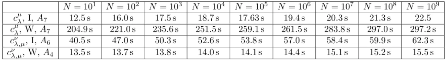
Tests were made with bi-processor PIII 1, 13GHz. The notation ”−” in an array means that we did not try the computation (and not that computation failed).
Recall (see for example [4] and [3]) that counting integral points in a lattice polytope is polynomial in the size of input if dimension is fixed, and NP-hard if dimension is not fixed. The figures 1 and 2 emphasizes this result.
In figure 1, the letter I stands for intermediate case (µ = [9N/10]θ for cµλand ν = 2[9N/10]θ for cν λ,µ),
while W stands for worst case (µ = 0 for cµλand ν = 0 for cνλ,µ).
N= 101 N = 102 N = 103 N = 104 N = 105 N = 106 N = 107 N = 108 N = 109 cµ λ, I, A7 12.5 s 16.0 s 17.5 s 18.7 s 17.63 s 19.4 s 20.3 s 21.3 s 22.5 cµ λ, W, A7 204.9 s 221.0 s 235.6 s 251.5 s 259.1 s 261.5 s 283.8 s 297.0 s 297.2 s cν λ,µ, I, A6 40.5 s 47.0 s 50.3 s 52.6 s 53.8 s 57.0 s 58.4 s 59.9 s 62.3 s cν λ,µ, W, A4 13.5 s 13.7 s 13.8 s 14.0 s 14.1 s 14.4 s 15.1 s 15.2 s 15.5 s
The computation can also be done with parameters, giving (N + 1)r(r−1)/2as expected.
Algebra Time Multiplicity c0
θ Time Polynomial N 7→ c 0 N θ A2 <0.1 s 2 = 2 1 < 0.1 s (N + 1)1 A3 <0.1 s 8 = 2 3 < 0.1 s (N + 1)3 A4 <0.1 s 64 = 2 6 < 0.1 s (N + 1)6 A5 0.4 s 1024 = 2 10 1.4 s (N + 1)10 A6 7.6 s 32768 = 215 36.2 s (N + 1)15 A7 169.3 s 2097152 = 2 21 2091 s (N + 1)21 A8 9401 s 268435456 = 228 − −
Figure 2: Multiplicity of 0 in V (N θ) when rank increases
Acknowledgements: Marc A. A. van Leeuwen explained me his software LıE and its internal mechanisms. Moreover, his competence in Maple has deeply influenced my method of programing.
References
[1] Baldoni-Silva W., De Loera J.A., and Vergne M., Counting Integer flows in Networks, available at math.ArXiv, CO/0303228. Program available at http://www.math.ucdavis.edu/∼totalresidue
[2] Baldoni-Silva W. and Vergne M., Residues formulae for volumes and Ehrhart polynomials of convex polytopes.manuscript 81 pages, 2001. available at math.ArXiv, CO/0103097.
[3] Barvinok A. and Pommersheim J., An algorithmic theory of lattice points in polyhedra, in: New Perspectives in Algebraic Combinatorics (Berkeley, CA, 1996-1997), 91-147, Math. Sci. Res. Inst. Publ. 38, Cambridge Univ. Press, Cambridge, 1999.
[4] Barvinok A., Lattice points and lattice polytopes, in Handbook of discrete and computational geometry, CRC Press Ser. Discrete Math. Appl., pages 133–152. CRC, Boca Raton, FL, 1997.
[5] De Loera J.A. and Sturmfels M., Algebraic Unimodular Counting, math.CO/0104286
[6] Van Leeuwen M. A. A., LiE, a software package for Lie group computations, Euromath Bull. 1 (1994), no. 2, p. 83–94.
[7] Szenes A. and Vergne M., Residue formulae for vector partitions and Euler-MacLaurin sums. preprint (2002), 52 pages. Available at math.ArXiv, CO/0202253.