HAL Id: hal-00296015
https://hal.archives-ouvertes.fr/hal-00296015
Submitted on 4 Sep 2006
HAL is a multi-disciplinary open access
archive for the deposit and dissemination of
sci-entific research documents, whether they are
pub-lished or not. The documents may come from
teaching and research institutions in France or
abroad, or from public or private research centers.
L’archive ouverte pluridisciplinaire HAL, est
destinée au dépôt et à la diffusion de documents
scientifiques de niveau recherche, publiés ou non,
émanant des établissements d’enseignement et de
recherche français ou étrangers, des laboratoires
publics ou privés.
the aerosol indirect effect
T. Storelvmo, J. E. Kristjánsson, G. Myhre, M. Johnsrud, F. Stordal
To cite this version:
T. Storelvmo, J. E. Kristjánsson, G. Myhre, M. Johnsrud, F. Stordal. Combined observational and
modeling based study of the aerosol indirect effect. Atmospheric Chemistry and Physics, European
Geosciences Union, 2006, 6 (11), pp.3583-3601. �hal-00296015�
© Author(s) 2006. This work is licensed under a Creative Commons License.
Chemistry
and Physics
Combined observational and modeling based study of the aerosol
indirect effect
T. Storelvmo1, J. E. Kristj´ansson1, G. Myhre1,2, M. Johnsrud2, and F. Stordal1 1Department of Geosciences, University of Oslo, Oslo, Norway
2Norwegian Institute for Air Research, Kjeller, Norway
Received: 16 January 2006 – Published in Atmos. Chem. Phys. Discuss.: 11 May 2006 Revised: 18 August 2006 – Accepted: 29 August 2006 – Published: 4 September 2006
Abstract. The indirect effect of aerosols via liquid clouds is investigated by comparing aerosol and cloud characteris-tics from the Global Climate Model CAM-Oslo to those ob-served by the MODIS instrument onboard the TERRA and AQUA satellites (http://modis.gsfc.nasa.gov). The compari-son is carried out for 15 selected regions ranging from remote and clean to densely populated and polluted. For each region, the regression coefficient and correlation coefficient for the following parameters are calculated: Aerosol Optical Depth vs. Liquid Cloud Optical Thickness, Aerosol Optical Depth vs. Liquid Cloud Droplet Effective Radius and Aerosol Op-tical Depth vs. Cloud Liquid Water Path. Modeled and ob-served correlation coefficients and regression coefficients are then compared for a 3-year period starting in January 2001. Additionally, global maps for a number of aerosol and cloud parameters crucial for the understanding of the aerosol indi-rect effect are compared for the same period of time. Signif-icant differences are found between MODIS and CAM-Oslo both in the regional and global comparison. However, both the model and the observations show a positive correlation between Aerosol Optical Depth and Cloud Optical Depth in practically all regions and for all seasons, in agreement with the current understanding of aerosol-cloud interactions. The correlation between Aerosol Optical Depth and Liquid Cloud Droplet Effective Radius is variable both in the model and the observations. However, the model reports the expected neg-ative correlation more often than the MODIS data. Aerosol Optical Depth is overall positively correlated to Cloud Liq-uid Water Path both in the model and the observations, with a few regional exceptions.
Correspondence to: T. Storelvmo ([email protected])
1 Introduction
Atmospheric particles play an important role in the atmo-sphere both through their ability to scatter and absorb solar radiation and through their fundamental role in cloud micro-physics. Without the presence of atmospheric aerosols, for-mation of clouds would require supersaturations which can only be realized under laboratory conditions and do not occur in the atmosphere. Water-soluble aerosols enable cloud for-mation at supersaturations typically found in the atmosphere, enabling water vapor to condense onto the particles. As the concentration of water soluble aerosols (also called Cloud Condensation Nuclei, CCN) increases, the Cloud Droplet Number Concentration (CDNC) increases and the average cloud droplet becomes smaller if the amount of cloud wa-ter remains constant. In other words, a negative correlation between aerosol number concentration and cloud droplet ef-fective radius (CER) is expected for clouds with comparable water content. This effect is often referred to as the “first aerosol indirect effect” or “Twomey effect” (Twomey, 1977). A second effect of an increase in CDNC and a correspond-ing decrease in CER is that the occurrence of CER above the threshold for efficient precipitation formation becomes less frequent (Rosenfeld et al., 2002), leading to a suppression of precipitation, and hence an increased liquid water content (LWC) and/or cloud cover (Kaufman and Koren, 2006). This effect is called the “second aerosol indirect effect” or “Al-brecht effect” (Al“Al-brecht, 1989). It implies that there should be a positive correlation between aerosol number concentra-tion and the liquid water content (LWC) or liquid water path (LWP=LWC·1Z, where 1Z is the cloud layer geometrical thickness).
Liquid water path and cloud droplet effective radius are related to cloud optical thickness (τc)through the following approximation (e.g. Liou, 1992):
τc ≈ 3 2 ·
LWP
Following this approximation, an increase in aerosol num-ber concentration should lead to an increase in cloud optical thickness through both the first and second aerosol indirect effect.
When focusing on water clouds only, an increase in cloud optical thickness will primarily lead to a negative shortwave cloud forcing at the top of the atmosphere (TOA) through an increase in cloud albedo. The mechanisms described above have received considerable attention in the scientific commu-nity lately due to the significant negative radiative forcing po-tentially associated with an increase in global aerosol burden due to anthropogenic activity (Lohmann and Feichter, 2005). The aerosol species which have increased in concentration since preindustrial times are mainly sulfate, black carbon and organic carbon, especially in connection to fossil fuel com-bustion and biomass burning.
While sulfate particles are highly hygroscopic and fre-quently act as CCN, black carbon is practically hydropho-bic, implying that the ability of black carbon (BC) to act as CCN is fairly poor. However, when internally mixed with for example sea salt or sulfate, BC can still take part in cloud droplet activation. Organic aerosols are generally a complex mixture of hundreds or even thousands of different organic compounds with varying hygroscopic properties (Kanakidou et al., 2005).
How aerosols affect the global radiative balance via clouds is still highly uncertain (Penner et al., 2001; Lohmann and Feichter, 2005), and a better understanding is crucial for the ability to predict future climate. Estimates vary by more than an order of magnitude between different General Circula-tion Models (GCMs). This study is an attempt to validate model parameterizations of how aerosols affect clouds in one GCM against satellite observations. Studies of how aerosol parameters relate to cloud parameters have previously been carried out by for example Nakajima et al. (2001), Quaas et al. (2004), Br´eon et al. (2002), Sekiguchi et al. (2003) and Wetzel and Stowe (1999). Nakajima et al. (2001) studied the relationships between column aerosol particle number (Na) and LWP, Cloud Optical Depth (COD) and CER from four months of AVHRR remote sensing in 1990. Nawas derived from the measured Aerosol Optical Depth (AOD) and the
˚
Angstr¨om exponent α. They found a positive correlation be-tween Naand COD, a negative correlation between Na and CER and no correlation between Na and LWP. Sekiguchi et al. (2003) found qualitatively similar correlations for Navs. CER and Navs. AOD in AVHRR and POLDER data. These results were used to evaluate the aerosol indirect effect to be about −0.6 W/m2 to −1.2 W/m2. Quaas et al. (2004) com-pared the relationships between the aerosol index (AI) and CER and AI vs. LWP from the POLDER-1 instrument and the Laboratoire de M´et´eorologie Dynamique-Zoom (LMDZ) general circulation model. The comparison was carried out for an eight month period in 1996–1997. A positive correla-tion was found between AI and LWP, and a negative corre-lation between AI and CER both in the observations (first
reported by Br´eon et al., 2002) and in the model. Quaas et al. (2006) used MODIS data to constrain the two gen-eral circulation models LMDZ and ECHAM4, resulting in an aerosol indirect effect of −0.5 W/m2and −0.3 W/m2, re-spectively. Wetzel and Stowe (1999) studied the relation-ships AOD vs. CER and AOD vs. COD in the NOAA polar-orbiting satellite advanced very high resolution radiome-ter (AVHRR) Pathfinder Atmosphere (PATMOS) data. The study was carried out for marine stratus clouds only. They found that CER decreased as AOD increased, and that AOD and COD were positively correlated.
In this study we compare model results and MODIS data, which are believed to be superior to previous satellite obser-vations of cloud parameters. We have chosen three sets of parameters in this study: Aerosol Optical Depth (AOD) vs. CER, AOD vs. LWP and AOD vs. COD. We have chosen to use AOD as a surrogate for aerosol number concentration, and calculate regression coefficients for each set of variables for both modeled and observational data. These regression coefficients, hereafter referred to as slopes, are calculated for daily instantaneous values for a 3 year period (2001–2003). Based on the previous reasoning, our working hypothesis in this study is that there is an overall negative correlation be-tween AOD and CER, and an overall positive correlation for AOD vs. LWP and AOD vs. COD. However, these relation-ships are not determined by aerosol-cloud interactions alone. Meteorological conditions can in certain regions lead to rela-tionships which do not support our hypothesis, while in other regions we can get the right relationship for the wrong rea-son with respect to the hypothesis. For example if a region is influenced by an air mass that is clean and moist compared to average conditions in this region, the AOD vs. LWP re-lationship is likely to be negative. Similarly, if a region is influenced by dry desert air masses with heavy dust aerosol loading, the AOD vs. CER relationship is likely to be nega-tive, but not as a result of aerosol-cloud interactions. Hence, one has to be very careful when drawing conclusions based on the modeled and observed relationships. Yet other fac-tors than the meteorology can also influence the relation-ships. We will come back to this in Sect. 6. We also per-form a global comparison between CAM-Oslo and MODIS for AOD, CER, COD, LWP and cloud fraction (CFR).
The following section (Sect. 2) contains a short descrip-tion of CAM-Oslo and the framework for calculadescrip-tions of the aerosol indirect effect. Storelvmo et al. (2006) contains a more detailed description of this framework. Section 3 con-tains a description of the MODIS instrument placed onboard the TERRA and AQUA satellites and its retrieval methods.
Extensive comparisons between MODIS and CAM-Oslo will be presented in Sect. 4 for the selected regions and pa-rameter sets, while comparisons of global maps and averages are given in Sect. 5. Our conclusions are given in Sect. 6.
2 Model description
The modeling tool in this study, CAM-Oslo, is a modified version of the National Center for Atmospheric Research (NCAR) Community Atmosphere Model Version 2.0.1 (CAM 2.0.1) (http://www.ccsm.ucar.edu/models/atm-cam).
For this study, the model was run with an Eulerian dy-namical core, 26 vertical levels and T42 (2.8◦×2.8◦) hor-izontal resolution. We run the model with climatological Sea Surface Temperatures (SSTs). Alternatively, one could also force the model to reproduce observed meteorological conditions corresponding to the time period of our MODIS observations. As the purpose of this study is to investi-gate relationships between aerosol and cloud parameters typ-ical for different regions and seasons rather than relation-ships in specific time periods, we have not taken this ap-proach here. The model is run with an interactive lifecycle model for sulfate and carbonaceous aerosol species (Iversen and Seland, 2002), with emissions corresponding to present-day (AEROCOM B emissions, http://nansen.ipsl.jussieu.fr/ AEROCOM). These are hereafter combined with dust and sea salt background aerosols in multiple lognormal aerosol modes (Kirkev˚ag and Iversen, 2002; Kirkev˚ag et al., 2005). The Cloud Droplet Number Concentration (CDNC) is pre-dicted in the model using a prognostic equation with micro-physical source and sink terms for CDNC. CDNC can be lost through evaporation, precipitation processes (divided into autoconversion, accretion by rain and accretion by snow), selfcollection (the process by which droplets collide and stick together without forming precipitation) and freezing.
The source term is determined using a scheme devel-oped by Abdul-Razzak and Ghan (2000) for activation of Cloud Condensation Nuclei to form cloud droplets. A de-tailed description of the framework for calculation of the Aerosol Indirect Effect in CAM-Oslo is given in Storelvmo et al. (2006). With the current model setup the change in shortwave cloud forcing at the top of the atmosphere due to the first and second aerosol indirect effect is −0.38 W/m2. In this study we assumed a model spin-up of four months, after which we ran the model for 3 years. For the regional comparison, the calculations of slopes and correlation coef-ficients are based on daily instantaneous values from these three years. For the global comparison, global maps and av-erages are based on monthly means from the same period.
3 Modis description
MODIS, a 36-band scanning radiometer, is a key instrument onboard the Terra (EOS AM) and Aqua (EOS PM) satel-lites. Terra was launched in December 1999, while Aqua was launched in May 2002. The cloud retrieval (Platnick et al., 2003) for optical depth and effective radius is derived from a set of bands with no absorption (0.65, 0.86 and 1.2 µm) and water absorption (1.6, 2.1 and 3.7 µm). The non-absorbing
bands give most information about the cloud optical depth, whereas the absorbing bands are most important for infor-mation on effective radius. The sets of bands that are used depend on the underlying surface. The MODIS liquid water path (LWP) is obtained from CER and COD from the rela-tionship given in Eq. (1).
For Aerosol Optical Depth (AOD) retrieval, the algorithm is different over land and ocean surfaces and described in Kaufman et al. (1997) and Tanr´e et al. (1997), respectively. An overview of the two retrievals and updated information on the retrieval algorithms are given in Remer et al. (2005). Over the ocean, pre-calculated look-up tables (LUT) are used in combination with the assumption of a bi-modal log-normal aerosol size distribution. As nucleation mode parti-cles are too small to be detected, tropospheric aerosols are described by one accumulation mode and one coarse mode. The measured spectral radiances are compared to the pre-calculated values from LUT to obtain the best fit. The spec-tral bands used for remote sensing of aerosols over ocean are 0.55 µm, 0.659 µm, 0.865 µm, 1.24 µm, 1.64 µm and 2.13 µm.
Over land it is difficult to distinguish the reflectance from the surface and from the aerosols. In MODIS the 2.13 µm band is used to estimate the surface reflectance in the visible part. Thereafter, aerosol optical depth is determined based on the use of LUT. There are four possible aerosol types over land: Continental aerosol, Biomass burning aerosol, Indus-trial/urban aerosol and Dust aerosol. In all cases multimodal lognormal size distributions are assumed.
More detailed information on algorithms for retrieval of aerosol- and cloud parameters can be found on http: //modis-atmos.gsfc.nasa.gov.
In this study, we have used MODIS data from the Terra platform for a three-year time period, from 2001 to 2003. The data is interpolated in space to a 1◦×1◦grid, while the temporal resolution of 24 h allows for only one satellite over-pass. For the regional study we have neglected AODs lower than 0.01 and higher than 1, based on the reasoning of Remer et al. (2005).
4 Regional comparison 4.1 Method
In order to test our working hypothesis presented in Sect. 1, we compare the slopes for AOD vs. CER, AOD vs. LWP and AOD vs. COD calculated from MODIS data and CAM-Oslo data. These slopes are calculated for the linear regression of all data points within each of the 15 regions for each month of the year. For each slope that we calculate we also determine the degree of statistical significance for the given relation-ship. This is done by running a two-tailed t-test and imposing constraints of significance at the 0.10 and 0.01 levels, assum-ing independence among the data points. Based on this, we
Fig. 1. The 15 selected regions. 0.0 0.2 0.4 0.6 0.8 1.0 AOD 0.0 5.0 10.0 15.0 20.0 25.0 30.0 CER (um) Europe, January
Aerosol Optical Depth vs. Cloud Effective Radius MODIS data CAM−Oslo data Linear regr.−MODIS Linear regr.−CAM−Oslo
Fig. 2. Cloud effective radius as a function of Aerosol Optical
Depth for Europe in January for both MODIS and CAM-Oslo data.
divide the statistical significance into three categories, repre-senting no, medium and high statistical significance. The cat-egories can be recognized in the Tables 1–3 as regular num-bers (Cat. 1), bold numnum-bers (Cat. 2) and red bold numnum-bers (Cat. 3). As the total number of data points is in most cases several thousand, we believe that the number of independent data points is generally high. As linearity between AOD and CER, COD and LWP cannot necessarily be expected from theory, we have also studied other relationships for each pair of parameters. This issue will be discussed further in Sect. 6.
0.0 0.2 0.4 0.6 0.8 1.0 AOD 0.0 5.0 10.0 15.0 20.0 25.0 30.0 CER (um)
Southwest Africa, July
Aerosol Optical Depth vs. Cloud Effective Radius MODIS data CAM−Oslo data Linear regr.−MODIS Linear regr.−CAM−Oslo
Fig. 3. Cloud effective radius as a function of Aerosol Optical
Depth for Southwest Africa in July for both MODIS and CAM-Oslo data.
4.2 Regional relationships between AOD and CER, LWP and COD
The regions selected for comparison of AOD, LWP, COD and CER are listed below with a discussion of the modeled and observed slopes for the three parameter sets. A global map displaying the 15 selected regions is shown in Fig. 1. Results of the comparison are given in Tables 1–3 for each month of the year, and selected examples are shown in Figs. 2–7.
Table 1. Slopes for Aerosol Optical Depth (AOD) vs. Cloud droplet effective radius (CER) for each region and each month of the year
calculated based on 3 years of daily instantaneous values for the MODIS instrument and CAM-Oslo. Bold red numbers represent strong statistical significance, bold black numbers indicate moderate statistical significance. Statistical significance is otherwise low.
Region Jan Feb March April May June July Aug Sep Oct Nov Dec Po CAM −2.95 −0.09 −7.32 −3.37 −5.13 −6.52 −9.81 −7.02 −8.33 −6.60 −5.81 −9.72 MODIS 1.55 −1.49 1.11 −1.19 −1.24 −0.95 −0.62 1.15 −0.83 1.28 5.43 4.89 Pe CAM 11.8 11.4 −6.09 −4.53 1.92 −14.5 −12.1 −0.77 −6.14 16.1 19.0 23.6 MODIS −8.78 −8.65 −8.22 −12.2 −17.8 −15.9 −18.7 −13.0 −13.6 −8.89 −9.57 −8.33 EUS CAM 0.47 −0.11 −2.68 −5.15 −5.38 −10.0 −9.68 −11.6 −12.2 −11.7 −2.65 0.85 MODIS 5.62 5.37 5.13 7.26 5.85 5.02 4.34 5.26 6.13 4.87 2.72 2.91 NAB CAM −16.4 −17.1 −17.2 −16.2 −17.1 −12.6 −3.13 2.83 −3.31 −14.6 −17.9 −18.3 MODIS −5.17 −5.443 −5.12 −3.30 −3.76 −5.31 −4.55 −4.40 −4.78 −9.46 −4.12 −2.58 An CAM −9.70 −10.5 −10.9 −11.3 −16.0 9.95 13.6 14.8 0.00 5.19 −11.9 −5.15 MODIS −11.0 −9.81 −13.9 −19.6 −21.2 −25.2 −18.5 −15.1 −7.35 −6.51 −11.4 −10.2 Eu CAM −8.77 −7.64 −7.67 −8.08 −11.3 −7.67 −10.5 −12.0 −14.4 −9.00 −5.97 −6.55 MODIS −1.54 0.49 1.51 1.06 2.35 0.67 −0.04 −0.54 0.96 1.89 1.27 0.95 Ch CAM 5.08 1.22 3.13 3.38 3.81 2.87 −0.60 0.39 3.56 2.94 3.29 3.97 MODIS 3.92 2.60 3.51 2.28 2.23 1.72 1.14 1.62 2.18 3.54 3.85 2.40 Ma CAM −6.64 −7.98 −12.4 −9.06 −7.84 −5.73 −7.27 −2.58 7.00 4.36 −7.67 −9.08 MODIS −17.4 −16.6 −14.9 −12.5 −9.47 −6.15 −1.97 −1.20 −5.01 −16.9 −13.9 −8.20 Ke CAM −15.7 −15.9 −13.2 −13.1 −12.3 −11.6 −11.9 −11.9 −14.4 −12.6 −16.8 −15.5 MODIS 3.98 3.54 3.53 −0.62 −4.81 −0.32 −7.25 −3.78 −0.66 1.19 6.70 5.47 Cal CAM 1.24 −4.92 −21.3 −23.6 −7.39 −14.0 −27.4 −0.04 -17.1 −2.01 −4.55 −4.58 MODIS −4.91 −2.25 −1.79 1.40 2.35 3.56 2.50 2.32 1.92 2.65 −3.27 −4.97 CSA CAM −8.48 −6.92 −8.92 −8.01 −20.5 −41.2 −35.3 −21.8 −24.1 −40.3 −34.7 −22.5 MODIS 0.98 2.21 3.38 8.15 8.72 8.52 4.61 5.30 4.07 4.16 6.35 3.94 Sah CAM −4.00 0.65 −18.3 −2.44 −7.69 −20.4 -15.4 −8.54 −0.91 −6.77 −7.44 −20.7 MODIS 2.14 1.33 −1.42 0.80 −0.46 −3.09 −4.90 −5.66 −6.09 −2.12 −0.22 3.97 SWA CAM −9.85 −0.01 17.9 22.3 21.5 −5.01 −13.6 −13.2 −15.7 −24.6 −7.82 −9.63 MODIS 3.56 1.15 −3.97 −4.78 −6.30 −7.91 −5.56 −3.51 −0.21 −0.51 3.21 3.21 CAf CAM −13.5 −11.7 −10.4 3.66 −9.76 −10.5 −9.66 −11.3 −12.1 −19.0 3.03 7.86 MODIS −2.73 −1.00 −1.08 1.31 1.13 1.43 1.67 3.74 3.91 3.08 3.15 0.71 In CAM −9.72 −15.2 −15.8 −8.16 −7.28 −13.2 −10.9 −6.08 −4.07 −1.85 −17.5 −22.8 MODIS −4.61 −6.40 −7.24 −10.9 −9.10 −5.21 −6.26 −6.06 −5.35 −5.50 −8.39 −5.64
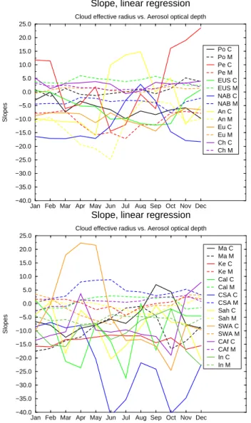
The slopes for AOD vs. CER and AOD vs. COD are also given as a function of calendar month for all regions in Figs. 8 and 9, respectively. The larger variability in CAM-Oslo compared to the MODIS data is evident in both figures. Each slope is calculated based on daily instantaneous val-ues from all three years for the calendar month considered. This is done to ensure a sufficient number of data points for the slopes to be reliable and to be able to reduce the influ-ence of features specific for one particular year. In general, the model (red dots) is not able to reproduce the variabil-ity in AOD found in the satellite data (black dots). This is to be expected, as we run the model with prescribed back-ground aerosol. The underestimation of AOD variability is
particularly evident for remote regions far from the aerosol sources, as can be seen in Fig. 3 for Southwest Africa and in Fig. 7 for the Angola Basin. Variability in LWP is high and possibly overestimated in the model, at least at the high end. Consequently, the modeled slopes for AOD vs. LWP and AOD vs. COD are much steeper than the corresponding MODIS slopes. This issue will be discussed in more detail in Sect. 6. In the discussion below, we have chosen to focus on the sign and statistical significance for each parameter set. The results discussed below are given in Table 1 for the rela-tionship AOD vs. CER, Table 2 for the relarela-tionship AOD vs. COD and Table 3 for the relationship AOD vs. LWP.
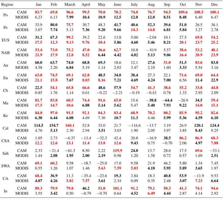
Table 2. Slopes for Aerosol Optical Depth (AOD) vs. Cloud Optical Depth (COD) for each region and each month of the year calculated
based on 3 years of daily instantaneous values for the MODIS instrument and CAM-Oslo. Bold red numbers represent strong statistical significance, bold black numbers indicate moderate statistical significance. Statistical significance is otherwise low.
Region Jan Feb March April May June July Aug Sep Oct Nov Dec
Po CAM 83.7 69.8 96.6 99.5 70.0 70.2 74.8 76.7 94.5 109.6 108.5 100.1 MODIS 6.23 6.13 7.99 10.4 10.9 12.5 12.0 12.0 8.51 8.48 6.40 6.47 Pe CAM 33.9 80.0 75.7 30.7 48.3 41.7 40.6 52.3 39.6 51.0 26.5 36.1 MODIS 3.07 7.74 5.13 7.36 9.20 9.66 14.3 14.8 6.81 5.84 3.27 2.78 EUS CAM 31.2 67.3 99.2 39.2 22.6 13.8 5.06 −2.04 10.1 27.5 69.8 54.2 MODIS 17.5 12.3 9.13 9.76 10.4 5.86 4.60 5.46 8.21 20.1 23.7 25.2 NAB CAM 53.4 73.0 75.2 47.0 36.6 62.7 10.8 −10.9 5.57 38.6 53.2 48.1 MODIS 21.9 17.9 12.8 8.52 6.44 4.42 4.02 5.13 9.06 16.4 20.9 23.9 An CAM 60.0 63.7 74.0 68.8 69.3 18.6 12.1 27.6 51.0 51.5 83.6 83.8 MODIS 4.58 2.20 6.84 5.19 1.14 2.03 3.47 2.10 1.60 3.33 5.54 3.16 Eu CAM 63.0 74.5 69.1 62.8 48.5 34.0 38.4 27.3 22.1 71.6 69.0 64.4 MODIS 21.1 15.8 7.67 8.03 8.16 7.21 4.69 4.24 7.00 6.56 11.4 22.9 Ch CAM 22.5 54.1 65.8 66.6 48.6 57.9 54.7 41.3 38.6 55.2 33.8 44.8 MODIS 0.85 1.76 1.14 0.61 −0.22 −2.21 −0.19 −0.43 0.78 1.33 2.95 2.09 Ma CAM 81.7 83.8 60.5 74.4 91.6 65.0 15.6 −38.8 −64.4 −26.9 34.5 59.4 MODIS 17.5 14.7 10.6 6.88 5.14 5.62 5.47 5.40 7.93 9.22 14.0 15.1 Ke CAM 84.8 97.0 91.5 92.1 84.3 83.4 68.9 70.2 80.2 85.9 95.2 82.6 MODIS 6.30 6.44 6.08 4.69 7.30 10.7 11.3 4.46 5.99 5.36 4.59 6.10 Cal CAM 114.5 154.7 160.1 52.8 33.0 21.7 −116.6 −13.7 3.19 26.9 120.1 124.4 MODIS 4.76 5.13 2.30 2.94 3.51 3.03 1.90 2.05 3.97 3.85 8.43 9.25 CSA CAM 1.05 2.73 −6.37 −13.4 −32.3 42.4 20.8 −16.9 38.5 86.2 86.9 68.3 MODIS 12.2 12.6 13.1 11.4 13.8 12.6 9.43 0.75 −0.70 2.06 4.97 7.88 Sah CAM 2.33 −21.4 −61.3 8.50 2.22 119.9 24.0 13.7 28.6 17.5 69.6 −33.1 MODIS 1.44 2.08 1.95 2.00 2.19 0.98 1.20 1.58 0.72 0.57 1.69 2.51 SWA CAM 69.1 60.2 9.58 −18.7 −25.0 17.0 9.58 21.9 46.2 5.80 1.34 7.45 MODIS 0.55 1.26 1.07 1.46 5.63 7.59 5.83 4.18 5.95 5.89 3.65 1.97 CA CAM 68.4 36.9 11.3 −35.4 −23.6 19.3 3.84 18.3 40.8 53.9 −11.9 9.53 MODIS 4.07 4.26 5.82 7.57 3.61 2.34 0.09 0.35 2.48 3.07 7.23 6.64 In CAM 89.3 79.9 79.8 46.2 51.0 101.1 91.2 79.1 50.3 41.3 74.1 94.6 MODIS 3.55 3.42 0.50 −0.79 −0.70 0.64 4.52 6.49 4.44 2.87 4.14 2.92
– Polynesia (Po) (6◦S–35◦S, 170◦W–128◦W): This re-gion is expected to represent clean conditions in a trop-ical climate with monsoon rain in December through March. Sea salt is expected to be the predominant aerosol species. MODIS data show a relatively robust positive AOD vs. LWP relationship with moderate sta-tistical significance. This ensures a positive relationship between AOD and COD with an overall moderate sta-tistical significance, although no clear AOD vs. CER re-lationship is found. Qualitatively, similar rere-lationships are found in the model, although both the AOD vs. LWP and AOD vs. COD relationships are of stronger
statis-tical significance than the corresponding MODIS rela-tionships. A possible explanation for the strong AOD vs. LWP correlation is that the Albrecht effect often comes into play in this region, dominating the Twomey effect. However, there are also other possible explana-tions, as we will discuss in more detail in Sect. 6. – Peru Basin (Pe) (22◦S–1◦N, 110◦W–85◦W, ocean
only): Peru basin is a dry maritime region with sea-sonal influence by aerosols from biomass burning from May to August. MODIS data show a negative AOD vs. CER relationship which is overall of category 2 and
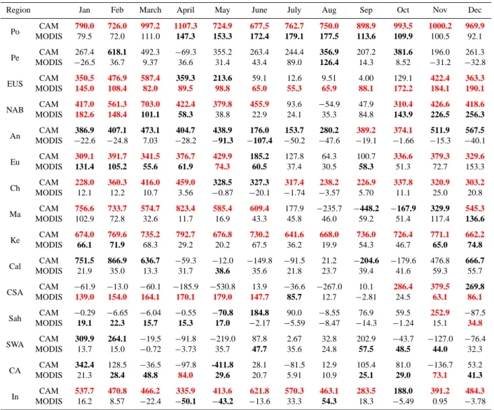
Table 3. Slopes for Aerosol Optical Depth (AOD) vs. Cloud Liquid Water Path (LWP) for each region and each month of the year calculated
based on 3 years of daily instantaneous values for the MODIS instrument and CAM-Oslo. Bold red numbers represent strong statistical significance, bold black numbers indicate moderate statistical significance. Statistical significance is otherwise low.
Region Jan Feb March April May June July Aug Sep Oct Nov Dec Po MODISCAM 790.079.5 726.072.0 997.2111.0 1107.3147.3 724.9153.3 172.4677.5 179.1762.7 177.5750.0 113.6898.9 109.9993.5 1000.2100.5 969.992.1
Pe CAM 267.4 618.1 492.3 −69.3 355.2 263.4 244.4 356.9 207.2 381.6 196.0 261.3 MODIS −26.5 36.7 9.37 36.6 31.4 43.4 89.0 126.4 14.3 8.52 −31.2 −32.8
EUS CAM 350.5 476.9 587.4 359.3 213.6 59.1 12.6 9.51 4.00 129.1 422.4 363.3 MODIS 145.0 108.4 82.0 89.5 98.8 65.0 55.3 65.9 88.1 172.2 184.1 190.1
NAB MODISCAM 417.0182.6 561.3148.4 703.0101.1 422.458.3 379.838.8 455.922.9 24.193.6 −35.354.9 84.847.9 143.9310.4 226.5426.6 418.6256.3
An MODISCAM −386.922.6 −407.124.8 473.17.03 −404.728.2 −438.991.3 −176.0107.4 −153.750.2 −280.247.6 −389.219.1 −374.11.66 −511.915.3 −567.540.1 Eu CAM 309.1 391.7 341.5 376.7 429.9 185.2 127.8 64.3 100.7 336.6 379.3 329.6 MODIS 131.4 105.2 55.6 61.9 74.3 60.5 37.4 30.5 58.3 51.3 72.7 153.3 Ch CAM 228.0 360.3 416.0 459.0 328.5 327.3 317.4 238.2 226.9 337.8 320.9 303.2 MODIS 12.1 12.2 10.7 3.56 −0.87 −20.1 −1.74 −3.57 5.70 11.1 25.0 20.8 Ma MODISCAM 756.6102.9 733.772.8 574.732.6 823.411.7 585.416.9 609.443.3 177.945.8 −46.0235.7 −59.2448.2 −51.4167.9 117.4329.9 545.3136.6 Ke MODISCAM 674.066.1 769.671.9 735.268.3 792.729.2 676.820.2 730.267.5 641.636.2 668.019.9 736.054.3 726.446.7 771.165.0 662.274.8 Cal CAM 751.5 866.9 636.7 −59.3 −12.0 −149.8 −91.5 21.2 −204.6 −179.6 476.8 666.7 MODIS 21.9 35.0 13.3 31.7 38.6 35.6 21.8 23.7 39.4 41.6 59.3 55.7 CSA CAM −61.9 −13.0 −60.1 −185.9 −530.8 13.9 −36.6 −267.0 10.1 286.4 379.5 269.8 MODIS 139.0 154.0 164.1 170.1 179.0 147.7 85.7 12.7 −2.81 24.5 63.1 86.1
Sah MODISCAM −19.10.29 −22.36.65 −15.76.04 −15.30.55 −17.070.8 −184.82.17 −90.05.59 −−8.478.55 −76.914.3 −59.51.24 252.915.1 −34.887.5
SWA MODISCAM 309.913.7 264.115.0 −−19.50.72 −−91.83.73 −35.7219.0 47.787.8 35.62.67 24.832.8 202.957.5 −48.543.7 −44.0127.0 −32.376.4
CA CAM 342.4 128.5 −36.5 −97.8 -411.8 28.1 −81.5 12.9 105.4 81.0 −136.7 53.2 MODIS 21.3 28.4 48.8 84.0 29.6 20.7 5.91 10.9 25.1 29.0 73.1 41.3 In CAM 537.7 470.8 466.2 335.9 413.6 621.8 570.3 463.1 283.5 188.0 391.2 484.3
MODIS 16.2 8.57 −22.4 −50.1 −43.2 −13.6 33.3 54.3 18.3 −5.49 0.95 −3.78
persistent over seasons and years. This ensures a pos-itive AOD vs. COD correlation, although the relation-ship AOD vs. LWP is variable and statistically insignif-icant. The model results show no clear relationship be-tween AOD and CER, and an overall positive corre-lation for AOD vs. LWP with variable statistical sig-nificance. The resulting AOD vs. COD relationship is always positive, but the statistical significance varies. Here, both MODIS and the model show a positive cor-relation between AOD and COD, but for different rea-sons.
– Eastern USA/Canada (EUS) (25◦N–50◦N, 60◦W– 95◦W, land only): Eastern USA and Southeast Canada has a typical humid mid-latitude climate and is a densely populated region with significant industrial
ac-tivity. MODIS data show a very strong positive corre-lation for AOD vs. LWP with strong statistical signif-icance. This leads to a positive correlation for AOD vs. COD of category 2 and 3. This happens despite the fact that AOD vs. CER is positively correlated, al-though with low statistical significance. CAM-Oslo shows a positive correlation between AOD and LWP, which is strongest in the winter. AOD vs. CER is neg-atively correlated in the summer, with moderate statis-tical significance. In winter the statisstatis-tical significance becomes weak. The resulting AOD vs. COD is overall positive, but with varying statistical significance. Fig-ure 4 shows COD as a function of AOD for February for both MODIS and CAM-Oslo. It illustrates that MODIS has a higher variability for AOD than the model, while
0.0 0.2 0.4 0.6 0.8 1.0 AOD 0.0 20.0 40.0 60.0 80.0 100.0 120.0 COD
Eastern USA, February
Aerosol Optical Depth vs. Cloud Optical Depth MODIS data CAM−Oslo data Linear regr.−MODIS Linear regr.−CAM−Oslo
Fig. 4. Liquid Cloud Optical Depth as a function of Aerosol Optical
Depth for Eastern USA in February for both MODIS and CAM-Oslo data.
CAM-Oslo has a higher variability than MODIS for COD. However, one must keep in mind that MODIS retrievals of AOD are less reliable over land than over ocean, in particular over bright surfaces. As this re-gion is largely covered by snow in winter, this may have affected the results. For this region, CAM-Oslo also has a stronger seasonal signal than MODIS. The model results are qualitatively similar to MODIS in winter. As this region is located in the Northern Hemisphere storm tracks, suppression of precipitation in connection to high aerosol loadings would not be surprising. – North American Basin (NAB) (25◦N–45◦S, 82◦W–
48◦W, ocean only): This region is marine, but strongly influenced by eastern USA pollution. In the MODIS data, AOD vs. CER and AOD vs. LWP are negatively and positively correlated, respectively. In both cases the statistical significance is relatively low, but they still act together (through Eq. 1) in causing a strong positive cor-relation for AOD vs. COD with moderate to strong sta-tistical significance. The model simulates a strong nega-tive AOD vs. CER relationship in winter, but no signifi-cant correlation in summer. The same seasonal variation can be seen for the positive AOD vs. LWP correlation. Consequently, AOD is positively correlated with COD, except in the summer months. Again, CAM-Oslo shows a seasonal signal which cannot be seen in the satellite data (Tables 1–3).
– Angola Basin (An) (25◦S–6◦S, 15◦W–15◦E, ocean only): This region is marine, but strongly influenced
0.0 0.2 0.4 0.6 0.8 1.0 AOD 0.0 20.0 40.0 60.0 80.0 COD India, September
Aerosol Optical Depth vs. Cloud Optical Depth MODIS data CAM−Oslo data Linear regr.−MODIS Linear regr.−CAM−Oslo
Fig. 5. Liquid Cloud Optical Depth as a function of Aerosol Optical
Depth for India in September for both MODIS and CAM-Oslo data.
by desert dust from North Africa and to some extent by organic carbon in the biomass burning season. In the satellite observation, there is a robust negative corre-lation between AOD and CER, and a positive but less statistically significant correlation between AOD and COD. There is no clear correlation between AOD and LWP. We believe this to be an example of how mete-orological conditions can lead to relationships which apparently are contradictory to our hypothesis (in this case that AOD and LWP are positively correlated). This does not imply that the hypothesis is wrong, but rather that aerosol-cloud interactions do not determine these relationships alone. Optically thin clouds with small droplets and low water content seem to be part of the explanation. These clouds seem to be present all year round and are possibly formed in continental air masses with high mineral dust loadings. In the model on the other hand, the AOD vs. CER correlation is variable both in sign and statistical significance. AOD vs. LWP is positively correlated with moderate statistical sig-nificance, and AOD vs. COD is always positive, but stronger in SH summer. This is another example of CAM-Oslo and MODIS both showing a positive cor-relation between AOD and LWP, but apparently for dif-ferent reasons. Figure 7 shows LWP as a function of AOD for MODIS and CAM-Oslo. The LWP range is practically the same for MODIS and the model, while the AOD range is much narrower for CAM-Oslo than for MODIS.
– Europe (Eu) (35◦N–55◦N, 10◦W–40◦E): Europe is densely populated and industrialized. Consequently, the region is dominated by sulfate and carbonaceous
0.0 0.2 0.4 0.6 0.8 1.0 AOD 0.0 200.0 400.0 600.0 800.0 LWP (g/m2)
Eastern China, November
Aerosol Optical Depth vs. Liquid Water Path MODIS data CAM−Oslo data Linear regr.−MODIS Linear regr.−CAM−Oslo
Fig. 6. Cloud Liquid Water Path as a function of Aerosol Optical
Depth for Eastern China in November for both MODIS and CAM-Oslo data.
aerosols, in addition to some Saharan dust. MODIS shows a relatively strong positive correlation for AOD vs. LWP leading to a positive correlation for AOD vs. COD. The relationship between AOD and CER is vari-able and has no statistical significance. Qualitatively, CAM-Oslo shows similar results, although the slopes are steeper, as discussed above. Figure 2 shows a rea-sonably good comparison between MODIS and CAM-Oslo for CER as a function of AOD for January. – Eastern China (Ch) (25◦N–47◦S, 100◦E–122◦E,
land only): This region is expected to be the most heavily polluted region, and soot aerosol concentrations are particularly high here. In this region MODIS shows overall varying correlations for all parameter sets, and the statistical significance is very low. This is slightly surprising, but can possibly be explained by the in-fluence of BC or by the so called “competition ef-fect” (Ghan et al., 1998). BC is a hydrophobic aerosol species, and hence does not act as a CCN. Conse-quently, one would not expect strong correlations be-tween AOD and CER/LWP/COD in regions with high BC concentration. In fact, the so called “semi-direct effect” (Hansen et al., 1997) can even lead to a LWP which decreases with increasing aerosol loading. This is supported by Kr¨uger and Graßl (2004), who found a reduction in the local planetary albedo due to aerosol absorption in clouds over China in long-term satellite observations. The fact that a cloud condensation nuclei must compete with all other CCN present for the avail-able water vapor is referred to as the competition effect.
0.0 0.2 0.4 0.6 0.8 AOD 0.0 100.0 200.0 300.0 400.0 LWP (g/m2)
Angola Basin, December
Aerosol Optical Depth vs. Liquid Water Path MODIS data CAM−Oslo data Linear regr.−MODIS Linear regr.−CAM−Oslo
Fig. 7. Cloud Liquid Water Path as a function of Aerosol Optical
Depth for Angola Basin in December for both MODIS and CAM-Oslo data.
In polluted areas like eastern China, the high number of CCN ensures that the supersaturation never reaches very high values. Hence, CDNC is non-linearly related to the number of CCN. The model shows the same weak AOD vs. CER correlation, but AOD is positively corre-lated with LWP and the statistical significance is high. Hence, the AOD vs. COD correlation is of category 2 and 3. Figure 6 shows LWP as a function of AOD for MODIS and CAM-Oslo. Again, the model never sim-ulates the extreme low and high values present in the MODIS data for AOD. For this region CAM-Oslo also simulates a somewhat higher cloud liquid water con-tent than MODIS. This region is an example of a case where the model possibly overestimates the influence from aerosols on precipitation release. As the model never reaches the high AOD values found in the MODIS data, the competition effect is possibly too weak in the model compared to the satellite.
– Mariana Basin (Ma) (10◦N–31◦N, 130◦E–165◦E): We consider this region a clean one, although its lo-cation downwind of the East-Asian sources may intro-duce some sulfate and carbonaceous aerosols. Mod-eled column burdens in this region are approximately 0.1 mg/m2, 0.5 mg/m2 and 1.0 mg/m2 for BC, OC and sulfate, respectively. In this region MODIS shows a strong negative correlation for AOD vs. CER, and a corresponding positive correlation for AOD vs. COD. However, in July–September the statistical significance is substantially reduced. A robust but statistically in-significant positive correlation for AOD vs. LWP is
Jan Feb Mar Apr May Jun Jul Aug Sep Oct Nov Dec −40.0 −35.0 −30.0 −25.0 −20.0 −15.0 −10.0 −5.0 0.0 5.0 10.0 15.0 20.0 25.0 Slopes
Slope, linear regression
Cloud effective radius vs. Aerosol optical depth
Po C Po M Pe C Pe M EUS C EUS M NAB C NAB M An C An M Eu C Eu M Ch C Ch M
Jan Feb Mar Apr May Jun Jul Aug Sep Oct Nov Dec
−40.0 −35.0 −30.0 −25.0 −20.0 −15.0 −10.0 −5.0 0.0 5.0 10.0 15.0 20.0 25.0 Slopes
Slope, linear regression
Cloud effective radius vs. Aerosol optical depth
Ma C Ma M Ke C Ke M Cal C Cal M CSA C CSA M Sah C Sah M SWA C SWA M CAf C CAf M In C In M
Fig. 8. Slopes for the linear regression of Aerosol Optical Depth
vs. Cloud Effective Radius for the 15 regions for both MODIS and CAM-Oslo.
found. AOD is weakly correlated with CER in the model. The AOD vs. LWP relationship is stronger, es-pecially in winter when the statistical significance is strong. Consequently, AOD is positively correlated with COD in NH winter. Again, both the model and MODIS show an overall positive correlation between AOD and COD, but apparently the Twomey effect is dominating in the satellite data, while the Albrecht effect is more important in the model.
– Kerguelen Plateau (Ke) (55◦S–40◦S, 45◦E–90◦E): This region is expected to be very clean as it is lo-cated far from anthropogenic sources. However, high seasalt concentrations are typically found at these lat-itudes, which are sometimes referred to as the
“Roar-Jan Feb Mar Apr May Jun Jul Aug Sep Oct Nov Dec
−20.0 0.0 20.0 40.0 60.0 80.0 100.0 Slopes
Slope, linear regression
Cloud optical depth vs. Aerosol optical depth
Po C Po M Pe C Pe M EUS C EUS M NAB C NAB M An C An M Eu C Eu M Ch C Ch M
Jan Feb Mar Apr May Jun Jul Aug Sep Oct Nov Dec
−100.0 −80.0 −60.0 −40.0 −20.0 0.0 20.0 40.0 60.0 80.0 100.0 120.0 140.0 160.0 Slopes
Slope, linear regression
Cloud optical depth vs. Aerosol optical depth
Ma C Ma M Ke C Ke M Cal C Cal M CSA C CSA M Sah C Sah M SWA C SWA M CA C CA M In C In M
Fig. 9. Slopes for the linear regression of Aerosol Optical Depth
vs. Cloud Optical Depth for the 15 regions for both MODIS and CAM-Oslo.
ing Fourties” and the “Furious Fifties” due to high wind speeds. In the MODIS data, a consistently positive but statistically insignificant correlation between AOD and LWP ensures positive correlation for AOD vs. COD (also weak). AOD vs. CER shows no statistical cor-relation at all. Differently from MODIS, CAM-Oslo simulates the expected correlations according to our hy-pothesis, all of strong statistical significance. In this re-gion, CAM-Oslo seems to simulate a stronger influence from aerosols on clouds than can be found in the satel-lite data. A possible explanation could be an underes-timation of the background aerosol load in the model. This would represent a stronger aerosol indirect effect, based on the reasoning that AIE shows saturation for higher aerosol loads.
– California (Cal) (30◦N–49◦N, 130◦W–112◦W, land only): This region is a combination of a typical west-coast climate with substantial marine influence to the west, and dry inland climate to the east. Big cities like San Fransisco and Los Angeles contribute with typi-cal urban aerosols. Aerosol types are typitypi-cally aerosols from fossil fuel burning with some dust and also sea salt from the ocean. MODIS data show a negative correla-tion between AOD and CER, and a positive correlacorrela-tion between AOD and LWP. However, none of the correla-tions are ever of higher statistical significance than cat-egory 2. The result is a positive AOD vs. COD corre-lation with low statistical significance. CAM-Oslo sim-ulates a consistently negative correlation between AOD and CER, but with variable statistical significance. The AOD vs. LWP relationship is variable both in sign and significance, implying that AOD is mostly positively correlated with COD, but with weak to moderate sta-tistical significance. AOD and LWP show a strong pos-itive correlation for December through March, but with no correlation for the rest of the year. The same is true for AOD vs. COD.
– Central South America (CSA) (20◦S–4◦S, 74◦W– 44◦W, land only): The region is associated with a wet tropical climate and extensive biomass burning in the dry season. In these periods organic aerosol con-centrations can be very high. MODIS shows a very strong positive and statistically significant relationship between AOD and LWP for this region. This leads to a positive correlation between AOD and COD, although AOD vs. CER is positively correlated. This positive correlation may be due to a strong Albrecht effect coun-teracting the Twomey effect. AOD and CER are neg-atively correlated in CAM-Oslo, the statistical signif-icance being particularly high in southern hemisphere (SH) spring.
– Western Sahara (Sah) (10◦N–28◦N, 20◦W–13◦E, land only): Sahara is the largest desert in the world, and the climate is very dry and dominated by dust aerosols. Both cloud fraction and frequency of cloud occurence are fairly low, so in this region correlations are calculated based on fewer data points than for other regions. MODIS shows variable relationships for both AOD vs. CER and AOD vs. LWP, and the statistical significance is low in both cases. The resulting corre-lation between AOD and COD is consistently positive, although the statistical significance is varying. As al-ready mentioned, MODIS AOD retrievals are less re-liable over bright surfaces, such as deserts. In CAM-Oslo, all correlations are variable both in sign and sta-tistical significance. As a high fraction of the aerosol loading is insoluble in this region, weak correlations be-tween AOD and cloud parameters should be expected.
– Southwest Africa (SWA) (6◦S–10◦N, 15◦W–13◦E): This region covers both land and ocean in a tropical wet climate. Dominating aerosol types are assumed to be sea salt, dust and periodically also organic carbon. MODIS correlations are comparable to those found for Western Sahara, and so are CAM-Oslo correlations. Figure 3 shows CER as a function of AOD for July for both satellite observations and model data. CAM-Oslo simulates slightly smaller cloud droplets than MODIS. In this region, AOD never reaches values higher than ∼0.5, while the highest AODs from MODIS are three times as high.
– India (In) (0◦N–22◦N, 68◦E–90◦E): India has a typ-ical monsoon climate with intense precipitation in sum-mer and dry conditions in winter. The region is densely populated and polluted with high concentrations of sul-fate and carbonaceous aerosols, especially in the dry season. In this region MODIS finds a robust negative correlation between AOD and CER with moderate sta-tistical significance. A robust positive correlation is also found for AOD vs. COD, but the statistical significance is lower due to a highly variable relationship between AOD and LWP. CAM-Oslo shows a robust negative AOD vs. CER correlation, a robust and strong positive AOD vs. LWP correlation and a strong positive AOD vs. COD correlation all of which agree with our work-ing hypothesis. Figure 5 shows COD as a function of AOD for this region for September from both the model and the observations.
– Central Africa (CAf) (12◦S–2◦N, 13◦E–35◦E): Central Africa is considered a tropical, wet climate, which experiences periods of heavy precipitation when the ITCZ shifts southwards during southern hemisphere summer. Dominant aerosol types are expected to be dust and carbonaceous aerosols from biomass burning. MODIS data show a strong positive correlation for AOD vs. LWP and AOD vs. COD, and the statistical signif-icance is overall of category 2. There is practically no correlation between AOD and CER. CAM-Oslo correla-tions are all variable in sign and statistical significance. Hence, in this region MODIS shows a stronger influence from aerosols on clouds than CAM-Oslo.
5 Global comparison
In this section, global maps of AOD, COD, CER, LWP and cloud fraction (CFR) are presented for both MODIS and CAM-Oslo as 3-year averages in Figs. 10–14, while global averages for the same parameters are given separately for land and ocean in Table 4.
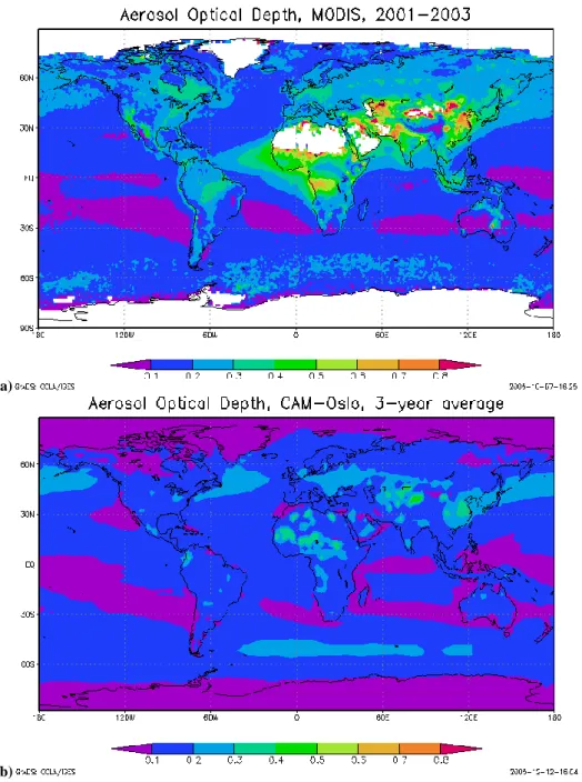
Figures 8a and b display AOD for MODIS and CAM-Oslo, respectively. Over the ocean, AOD from satellite and model
(a)
(b)
Fig. 10. Global maps of Aerosol Optical Depth from (a) MODIS and (b) CAM-Oslo.
compares very well. This indicates that the marine back-ground aerosol is realistic and that hygroscopic growth is well represented in the model. The only region where we see significant differences over ocean is the Atlantic Ocean, off the coast of North-Africa, where the model seems to grossly underestimate transport of Saharan dust and biomass burning aerosols. Over land we find significant differences between MODIS and CAM-Oslo, which are also evident in Table 4. Qualitatively, there are many similarities, but MODIS values are higher than CAM-Oslo values practically everywhere. There is a higher uncertainty associated with the MODIS
re-trieval algorithm for AOD over land than over ocean. There are indications that MODIS AOD is possibly overestimated (Remer et al., 2005). However, we still believe that the model underestimates continental aerosol concentrations.
Since the underestimation is also evident over continen-tal areas far from anthropogenic sources, it is possible that the background aerosol is too optically thin. Recently, it has been pointed out that primary biological aerosol particles (PBAPs) like bacteria, algae, dandruff etc. constitute a ma-jor portion of atmospheric aerosols (Jaenicke, 2005). Such aerosols are not included in the model simulation and could
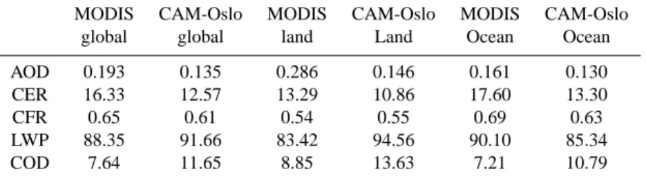
Table 4. Global, land and ocean averages of Aerosol Optical Depth (AOD), Cloud Droplet Effective Radius (CER), Cloud Fraction (CFR),
Liquid Water Path (LWP) and Liquid Cloud Optical Depth (COD).
MODIS CAM-Oslo MODIS CAM-Oslo MODIS CAM-Oslo global global land Land Ocean Ocean AOD 0.193 0.135 0.286 0.146 0.161 0.130 CER 16.33 12.57 13.29 10.86 17.60 13.30 CFR 0.65 0.61 0.54 0.55 0.69 0.63 LWP 88.35 91.66 83.42 94.56 90.10 85.34 COD 7.64 11.65 8.85 13.63 7.21 10.79
be part of the explanation for differences between satellite and model. Additionally, aerosols from biomass burning and fossil fuel burning seem to be somewhat underestimated in the model.
Figures 11a and b show CER for MODIS and CAM-Oslo, respectively. MODIS reports larger droplets than CAM-Oslo everywhere, with a global average of 16.33 µm. This is significantly higher than reported by for example Han et al. (1994) (11.4 µm) for the ISCCP dataset. Droplets are par-ticularly large over mid-oceanic areas where they frequently exceed 20 µm. The global average CER from the model is 12.57 µm. Compared to other GCMs predicting CER, this is actually a high number (e.g. Kristj´ansson, 2000 (10.31 µm), Ghan et al., 2001 (11.62 µm) and Lohmann et al., 1999 (ranging from 7.8 µm in NH winter over land to 11.9 µm in SH winter over oceans)). Such a large difference in CER will inevitably lead to significant differences in cloud radiative forcing. If models were to increase their cloud droplet sizes to MODIS values (∼30% increase in the case of CAM-Oslo) it would also have a notable effect on the predicted aerosol in-direct effect. We investigated this by running a Column radi-ation Model (CRM), which is a standalone version of the ra-diation code employed by NCAR CCM3, a previous NCAR model version (http://www.cgd.ucar.edu/cms/crm). We sim-ulated a cloud at 800 hPa covering a whole grid box lo-cated at the equator. Reducing cloud droplet effective ra-dius by 0.5 µm from 16.33 µm lead to a change in short-wave cloud forcing at the top of the atmosphere (TOA) of −3.75 W/m2. However, when reducing cloud droplet ra-dius by 0.5 µm from 12.57 µm, the corresponding change in shortwave cloud forcing at TOA is −4.45 W/m2, correspond-ing to a 20% larger indirect forccorrespond-ing.
It is also worth noting that the shortwave radiation scheme for liquid clouds applied in CAM-2.0.1 is unsuitable for droplets larger than 20 µm (Slingo, 1989). If the large droplets over ocean reported by MODIS are realistic, this scheme would need to be replaced or extended to be valid also for droplets as large as 30 µm. In Marshak et al. (2006) the effect of cloud horizontal inhomogeneity on retrievals of cloud droplet sizes is discussed as a factor possibly leading to overestimations.
The CER land-ocean contrast is larger in the MODIS data than for CAM-Oslo, the latter one being closer to the contrast reported by Han et al. (1994). However, both contrasts are pronounced, supporting the Twomey hypothesis.
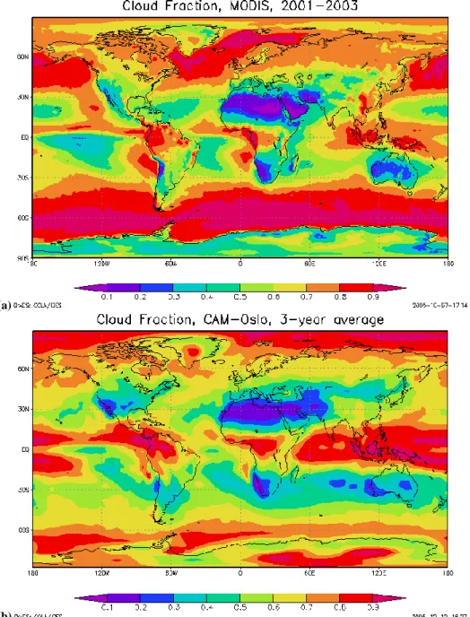
Total cloud fractions for (a) MODIS and (b) CAM-Oslo are given in Fig. 10. MODIS predicts a somewhat higher cloud fraction than CAM-Oslo, the global means being 65% and 61%, respectively. The underestimation in the model primarily takes place over the ocean, as apparent from the averages in Table 4. Figure 12 reveals that the cloud fraction over mid-latitude oceanic areas is significantly lower in the model than in the observations.
Figure 13 shows in-cloud liquid water path (LWP) for (a) MODIS and (b) CAM-Oslo. Both for the model and the ob-servations the in-cloud LWP is given as an average over all times, both when clouds are present and not. The global av-erage is very similar in CAM-Oslo and MODIS, as evident from Table 4. This indicates that the grid box averaged LWP would be somewhat higher for MODIS than for CAM-Oslo, as cloud fraction is higher in the MODIS data.
Figure 14 shows in-cloud optical depth (COD) (averaged over all times) for (a) MODIS and (b) CAM-Oslo. As the global mean in-cloud LWP is very similar in the model and the observations, the in-cloud COD should be somewhat higher in CAM-Oslo due to the smaller average CER. This is also the case for the global averages shown in Table 4.
We have left high latitudes out in the comparisons of LWP and COD, because we find these parameters unrealistically high in the MODIS data in these areas.
6 Discussion and conclusion
The way in which aerosols influence clouds, and how well modeled relationships between aerosol and cloud parameters compare to observations, have been investigated in this study. This was done on the regional scale by comparing the rela-tionships between parameters crucial in aerosol-cloud inter-actions, and on the global scale by comparing global maps and averages for the same parameters.
The regional study displayed fundamental differences be-tween modeled and observed relationships bebe-tween AOD
(a)
(b)
Fig. 11. Global maps of total cloud fraction from (a) MODIS and (b) CAM-Oslo.
and CER, AOD and LWP and AOD and COD. In the MODIS data, 96.1% of the calculated correlations for AOD vs. COD were positive, supporting but not necessarily confirming our aerosol-cloud hypothesis. For the strictest requirement (al-pha level of 0.01), 23.1% of the slopes were statistically sig-nificant. For a moderate requirement more typical for scien-tific studies (alpha level of 0.10), 61.8% of the slopes were statistically significant. CAM-Oslo gave a positive AOD vs. COD relationship in 90.0% of the cases. This is somewhat lower than MODIS, but the statistical significance was sig-nificantly higher in the model data. For the weakest
require-ment 71.6% of the slopes were statistically significant, while for the stricter requirement 50.6% were statistically signif-icant. The relationship AOD vs. CER is in the MODIS data highly variable both in sign and statistical significance, with 55.0% of the slopes being negative. Also in the model data the variability in AOD vs. CER is high, but a negative slope was found more often (80.6 % of the slopes) here than in the MODIS data. For an alpha level of 0.01, the frac-tions of negative slopes which were statistically significant are 13.1% and 15.9% for MODIS and CAM-Oslo, respec-tively. For an alpha level of 0.10, the corresponding numbers
(a)
(b)
Fig. 12. Global maps of Cloud Droplet Effective Radius from (a) MODIS and (b) CAM-Oslo.
are 46.5% and 42.1%. If we had calculated the slopes sepa-rately for cases with similar LWP, we would possibly find a stronger negative correlation. However, this was done in the study of Quaas et al. (2004) resulting in only slight changes. The AOD vs. LWP relationship shows the expected positive correlation more often, 80% and 82.8% in CAM-Oslo and MODIS data, respectively. However, this can not be inter-preted as an effect of aerosol-cloud interaction alone. Mete-orological conditions obviously play an important role. Hy-groscopic growth of aerosols is probably just as important. Water soluble aerosols grow due to humidity swelling, and
this growth is an increasing function of relative humidity. As aerosols grow due to water uptake, they become optically thicker. Relative humidity is assumed to be particularly high in the vicinity of clouds. Humid areas typically correspond to areas with high cloud water content. The mechanisms de-scribed above would lead to a positive correlation between AOD and LWP, and therefore also between AOD and COD. Hence, we can easily get such correlations for other reasons than the Albrecht effect. This issue is discussed in more detail in Myhre et al. (2006). For an alpha level of 0.01, 54.4% of the positive correlations are statistically significant
(a)
(b)
Fig. 13. Global maps of Liquid Water Path from (a) MODIS and (b) CAM-Oslo.
in CAM-Oslo, but the corresponding figure for MODIS is only 17.4%. For an alpha level of 0.10, corresponding num-bers are 74.3% and 45.6%, respectively.
It is interesting that AOD vs. COD shows a quite stable positive correlation despite the fact that the two parameters determining the COD according to Eq. (1) are relatively vari-able in their response to increasing AODs. Hence, it is tempt-ing to conclude that aerosols frequently influence the cloud optical depth through only one of the two main aerosol indi-rect effects. One can imagine that in regions with low pre-cipitation rates, the introduction of more cloud droplets will not affect precipitation release and hence not alter the water content of the clouds. Droplet sizes will however be sensitive to an increase in CCN and thereby CDNC. It is even possi-ble that cloud water will decrease as droplets become smaller and evaporate more easily.
Similarly, in regions where clouds frequently precipitate, an increase in CDNC can typically delay precipitation pro-cesses and allow clouds to last longer and contain more wa-ter (Andreae et al., 2004.) In these cases, droplet sizes may not be affected by the CDNC increase because cloud water is increasing too. Although MODIS and CAM-Oslo both show positive correlations between AOD and COD in most cases, they often do so for different reasons. Both the model and the satellite data indicate an aerosol effect on clouds, but for many regions they disagree in which of the two estab-lished aerosol indirect effects is likely to be more important. CAM-Oslo seems to slightly overestimate the aerosol effect on cloud droplet size compared to MODIS, and the model also seems to have a stronger seasonal variation than MODIS in many regions.
(a)
(b)
Fig. 14. Global maps of Liquid Cloud Optical Depth from (a) MODIS and (b) CAM-Oslo.
In our statistical analysis in Sect. 4, we made the basic assumption that there is a linear relationship between AOD and COD, CER and LWP. However, this can not necessar-liy be expected according to theory. For instance, if one assumes a linear relationship between aerosol number con-centration (ANC) and CDNC (from now on referred to as Assumption 1), this would imply an inverse relationship be-tween ANC and CER. To test this hypothesis, we calculated new correlation coefficients for the parameter set AOD (as a surrogate for ANC) vs. CER for both MODIS and CAM-Oslo data, this time based on an inverse relationship on the form CER=1/(a+b·AOD), where a and b are constants. While this approach led to similar or poorer correlation than the linear approach for the MODIS data, the opposite was true for the CAM-Oslo data. The expected relationship (i.e. CER decreasing with increasing AOD) was found more often (in
82.8% of the cases), and the statistical significance was a lot higher (29.8% for an alpha level of 0.01 and 49.1% for an alpha level of 0.10.
The competition effect is one reason why CDNC should not increase linearly with ANC, but rather reach a plateau for high aerosol loadings. If this effect is real, one would also expect to find plateau values for COD and LWP for high aerosol concentrations. We looked for such an effect in our model and satellite data by calculating new correlation coefficients for the parameter sets AOD vs. LWP and AOD vs. COD, this time based on a relationship on the form LWP/COD=c·AODd, where c and d are constants and d is between 0 and 1 (from now on Assumption 2). For the CAM-Oslo data, the correlation for this relationship was poorer than the linear one. For MODIS on the other hand, we found significant improvements: For AOD vs. COD, the expected
0.0 0.2 0.4 0.6 0.8 1.0 AOD 10.0 15.0 20.0 25.0 30.0 CER (um) CER vs. AOD Illustration Assumption 1 Assumption 2 Linear fit, assumption 1 Linear fit, assumption2
Fig. 15. CER vs. AOD for Assumption 1 and 2 and realistic
pro-portionality constants. Assumption 2 is clearly closer to a linear approximation than Assumption 1.
relationship was found in 96.1% of the cases, 39.3% of them being statistically significant for an alpha level of 0.01 and 76.3% being statistically significant for the weaker require-ment. For AOD vs. LWP, the corresponding figures were 88.9%, 32.5% and 66.9%, respectively.
Hence, there is a clear difference between the satellite and the model when it comes to what type of relationship gives the best correlation for each parameter set. We find this re-sult to be intriguing and propose the following explanation: Because MODIS AOD values are in most regions higher than those from CAM-Oslo, a saturation level for CDNC is reached more frequently. The saturation or plateau level can bee seen for COD and LWP in the satellite data. For CER, this saturation will lead to an inverse dependence of AOD which becomes closer to linearity. This is illustrated by Fig. 15 for realistic choices of proportionality constants. Possibly, we do not see the same effect in the CAM-Oslo data because high levels of aerosol loading are reached less frequently, or because of an underestimation of the compe-tition effect. If so, this would lead to an overestimation of the aerosol indirect effect in the model. Overestimations of the AIE compared to MODIS were also found in Quaas et al. (2006) for the LMDZ and ECHAM4 GCMs.
The global study revealed that AOD is significantly lower in CAM-Oslo than in MODIS over the continents. However, as the reliability of MODIS AOD retrievals over land is ques-tionable (Quaas et al., 2006) a quantification of this under-estimation cannot be given. The CAM-Oslo cloud fraction
is on global average only slightly lower than the MODIS cloud fraction. Global patterns are somewhat different, as CAM-Oslo overpredicts cloud cover in the tropics and un-derestimates mid-latitude oceanic cloud cover compared to MODIS.
CER is significantly smaller in CAM-Oslo than in MODIS. MODIS reports droplets larger than 22 µm over large oceanic areas in the tropics. If this is realistic, the crit-ical radius at which autoconversion is assumed to become efficient (15 µm) in CAM-Oslo must be reconsidered. The global comparison of LWP shows that CAM-Oslo slightly overpredicts LWP in the tropics. Otherwise, global patterns and global averages are quite similar. The COD is higher in CAM-Oslo than in MODIS in the global comparison. This is to be expected as LWP is slightly higher and CER is signifi-cantly lower in the model than in the MODIS retrievals.
This study only considers the relationship between AOD and cloud parameters for liquid clouds. A parameterization of aerosol influence on ice clouds is under development for CAM-Oslo, and will be compared to MODIS data in a simi-lar manner to that presented here. We firmly believe that it is important to validate not only global averages and spatial dis-tributions, but also instantaneous values in different regions, in order to achieve better understanding of how aerosols in-teract with clouds.
Acknowledgements. The work presented in this paper has been
supported by the Norwegian Research Council through the COM-BINE project (grant no. 155968/S30). Furthermore, this work has received support of the Norwegian Research Council’s program for Supercomputing through a grant of computer time. We are grateful to A. Kirkev˚ag, Ø. Seland and T. Iversen for their important roles in the CAM-Oslo model development. We are grateful to S. Ghan at the Pacific Northwest National Laboratory for making his droplet activation scheme available and for help in implementing it in CAM-Oslo. The MODIS data used in this study were acquired as part of the NASA’s Earth-Sun System Division and archived and distributed by the Goddard Earth Sciences (GES) Data and Information Services Center (DISC) Distributed Active Archive Center (DAAC). Finally, we would like to thank one anonymous reviewer for comments that led to major improvements of the paper. Edited by: W. Conant
References
Abdul-Razzak, H. and Ghan, S.: A parameterization of aerosol ac-tivation, 2. Multiple aerosol type, J. Geophys. Res., 105, 6837– 6844, 2000.
Albrecht, B. A.: Aerosols, cloud microphysics, and fractional cloudiness, Science, 245, 1227–1230, 1989.
Andreae, M. O., Rosenfeld, D., Artaxo, P., Costa, A. A., Frank, G. P., Longo, K. M., and Silvas-Dias, M. A. F.: Smoking rain clouds over the Amazon, Science, 303, 1337–1342, 2004.
Br´eon, F. M., Tanr´e, D., and Generoso, S.: Aerosol Effect on Cloud Droplet Size Monitored from Satellite, Science, 295, 834–838, 2002.