HAL Id: hal-02019678
https://hal.uca.fr/hal-02019678
Submitted on 14 Feb 2019
HAL is a multi-disciplinary open access
archive for the deposit and dissemination of
sci-entific research documents, whether they are
pub-lished or not. The documents may come from
teaching and research institutions in France or
abroad, or from public or private research centers.
L’archive ouverte pluridisciplinaire HAL, est
destinée au dépôt et à la diffusion de documents
scientifiques de niveau recherche, publiés ou non,
émanant des établissements d’enseignement et de
recherche français ou étrangers, des laboratoires
publics ou privés.
Autofunk, a fast and scalable framework for building
formal models from production systems
Sébastien Salva, William Durand
To cite this version:
Sébastien Salva, William Durand. Autofunk, a fast and scalable framework for building formal models
from production systems. 9th ACM International Conference on Distributed Event-Based Systems,
DEBS, Jul 2015, oslo, Norway. pp.193-204, �10.1145/2675743.2771876�. �hal-02019678�
Industry Paper: Autofunk, a fast and scalable framework
for building formal models from production systems.
Sébastien Salva
LIMOS - UMR CNRS 6158 Auvergne University, France
[email protected]
William Durand
Manufacture Francaise des Pneumatiques Michelin, France
[email protected]
ABSTRACT
This paper proposes a model inference framework for pro-duction systems distributed over multiple devices exchang-ing thousands of events. Buildexchang-ing models for such systems and keeping them up to date is time consuming and expen-sive, thus not adequately taken care of. Our framework, called Autofunk and designed with the collaboration of our industrial partner Michelin, combines formal model-driven engineering and expert systems to infer formal models that can be used to perform analyses, e.g. test case generation, or help diagnose faults in production by highlighting faulty behaviours. Given a large set of production events, we infer exact models that only capture the functional behaviours of a system under analysis. In this paper, we introduce and evaluate our framework on a real Michelin manufacturing system, showing that it can be used in practice.
Keywords
Model inference, STS, expert system, production system, event-driven system.
1.
INTRODUCTION
Models are essential while working on the design of com-plex systems to build reliable implementations. But, they are also particularly useful when systems reach maintenance cycle, easing comprehension of the overall design and de-scribing how these systems work under the hood. This is important because people who are responsible for maintain-ing or improvmaintain-ing systems are most likely not the same who designed and built them. It is nearly impossible for one per-son to know all the details related to a particular system, hence the need for creating and maintaining models. In the industry, building models for production systems, i.e. event-driven systems that run in production environments and are distributed over several devices and sensors, is fre-quent since these are valuable in many situations like test-ing and fault diagnosis for instance. Models may have been
Permission to make digital or hard copies of all or part of this work for personal or classroom use is granted without fee provided that copies are not made or distributed for profit or commercial advantage and that copies bear this notice and the full cita-tion on the first page. Copyrights for components of this work owned by others than ACM must be honored. Abstracting with credit is permitted. To copy otherwise, or re-publish, to post on servers or to redistribute to lists, requires prior specific permission and/or a fee. Request permissions from [email protected].
DEBS’15,June 29 - July 3, 2015, OSLO, Norway. Copyright 2015 ACM 978-1-4503-3286-6/15/06. . . $15.00. DOI: http://dx.doi.org/10.1145/2675743.2771876
written as storyboards or with languages such as the Unified Modelling Language (UML) or even more formal languages. Usually, these models are designed when brand-new systems are built. It has been pointed out by our industrial partner that production systems have a life span of many years, up to 20 years, and are often incrementally updated, but not their corresponding models. This leads to a major issue which is to keep these models up to date and synchronised with the respective systems. This is a common problem with documentation in general, and it often implies rather under-specified or not documented systems that no one wants to maintain because of lack of understanding.
In this paper, we focus on this problem for production sys-tems that exchange thousands of events a day. Model infer-ence, a.k.a. model learning or model reverse-engineering, is a recent research field that addresses this issue. Models are built from documentation or execution traces (sequences of observed events). Several approaches have been proposed for different types of systems, usually for GUI applications, e.g. desktop or mobile applications. However, we noticed that these approaches are not tailored to support produc-tion systems. From the literature, we deduced the following key observations:
• model inference approaches give approximate models capturing the behaviours of a system and more. In our context, we want exact models that could be used for regression test case generation and fault diagnosis, • most of these approaches perform active testing on
sys-tems to learn models. Applying active testing on run-ning systems is not possible since these must not be disrupted,
• production systems exchange thousands and thousands of events a day. Most of the model inference approaches cannot take such a huge amount of information to build models.
Based on these observations, we propose a pragmatic model inference approach that aims at building formal models de-scribing functional behaviours of a system. Our goal is to quickly build exact models from large amounts of produc-tion events. Execuproduc-tion speed takes an important place for building up to date models. Such models could also be used for diagnosis every time an issue would be experienced in production. The strong originality of our approach lies in
the combination of two domains for model inference: model-driven engineering and expert systems. We consider formal models and their definitions to infer models by means of dif-ferent transformations. But we also take into consideration the knowledge of human experts captured by expert sys-tems. Intuitively, our proposal emerges from the following idea: a human expert, who is able to conceive specifications, is also able to diagnose the behaviours of the corresponding implementation by reading and interpreting its events. His knowledge could then be formalised and exploited to auto-matically infer models. A part of our approach is based upon this notion of knowledge implemented with inference rules. The paper is structured as follows: Section 2 gives some research directions considered in model inference and ex-plains our choices regarding our design. Section 3 presents an overview of the framework of our approach, called Auto-funk. This work has been conducted in the context of pro-duction systems for one of the world’s leading tire manu-facturer Michelin. Therefore, we describe this context, its assumptions, and a case study. We give the theoretical as-pects of Autofunk in Section 4, and an empirical evaluation in Section 5. We conclude in Section 6.
2.
RELATED WORK
Several papers dealing with model generation approaches were issued in the last decade. We present here some of them related to our work, and introduce some key observa-tions. We only consider the approaches that infer models by observing the application behaviours at runtime, even though other papers, e.g. [13], propose to build models from documentation.
White-box techniques. Many works were proposed to infer specifications from source code or APIs, e.g. [12, 11]. Specifications are inferred in [11] from correct method call sequences on multiple related objects. The approach prepro-cesses method traces to identify small sets of related objects and method calls which can be analysed separately. The approach was implemented in a tool which supports more than 240 million runtime events. Other methods [3, 5] focus on mobile and web applications. They rely upon concolic testing to explore symbolic execution paths of an applica-tion and to detect bugs. These white-box approaches the-oretically offer good code coverage. However, the number of paths being explored concretely is limited to short paths only. Furthermore, the constraints must not be too complex for being solved. As a consequence, the code coverage of these approaches may be lower in practice, and models tend to be too detailed, thus hard to read.
Black-box automatic techniques. Many other methods [9, 10] were proposed to build models from event-driven ap-plications seen as black-boxes, e.g. desktop, web and more recently mobile applications. Such applications have GUIs to interact with users and which respond to user input se-quences. Automatic testing methods are applied to exper-iment such applications through their GUIs to learn mod-els. For instance, Memon et al. [9] introduced the tool GUITAR for scanning desktop applications. This tool pro-duces event flow graphs and trees showing the GUI execu-tion behaviours. The tool Crawljax [10], which is specialised in AJAX applications, produces state machine models to
capture the changes of DOM structures of web documents by means of events (click, mouseover, etc.). To prevent a state space explosion, these approaches [9, 2] require state-abstractions specified by users, and given in a high level of abstraction. This decision is particularly suitable for com-prehension aid, but these models often lack information for test case generation. In contrast, other approaches try to reduce models on the fly. The algorithm introduced in [10] reduces the model size by concatenating identical states of the model under construction. But this cannot be gener-ically applied on all applications, and a state abstraction definition must be manually given.
Active learning. TheL∗algorithm [4] is still widely con-sidered with active learning methods for generating finite state machines. The learning algorithm is used in conjunc-tion with a testing approach to learn models, and to guide the generation of user input sequences based on the model. The testing engine aims at interacting with the application under test to discover new application states, and to build a model accordingly. If an input sequence contradicts the learned model, the learning algorithm rebuilds a new model that meets all the previous scenarios. This approach has successfully been applied to various domains from network protocol inference to mobile applications [8, 6].
Based on these works, we concluded that active methods cannot be applied on production systems. In our context, we only assume having a set of events passively collected, i.e. collected without disrupting the system. Furthermore, the event set may be vast. We observed that most of the previous methods are not tailored for supporting large scale systems and thus millions of events. Only a few of them, e.g. [11], can take huge event sets as input and still infer models quickly. Likewise, the previous techniques often leave aside the notion of correctness regarding the learned models, i.e. whether these models only express the observed behaviours while testing one or more behaviours. The approaches [8, 6] based upon theL∗learning algorithm [4] do not aim at yield-ing exact models. The others use abstraction mechanisms to reduce model sizes. For comprehension aid, an exact model is not mandatory but the model correctness is extremely im-portant if the model is later used for analysis purpose. In the case of production systems, it is highly probable that executing incorrect test cases can raise false positives, and it may even lead to severe damages on the devices.
That is why we propose a framework that aims at inferring models from collected events as in [11], but similarities end here. We focus on exact and formal model generation, us-ing expert systems and inference rules to emulate human knowledge, and transition systems to embrace formal tools.
3.
OVERVIEW
3.1
Context and assumptions
Michelin is a worldwide tire manufacturer and designs mos of its factories, production systems, and software by itself. Like many other industrial companies, Michelin follows the Computer Integrated Manufacturing (CIM) approach, using computers and software to control the entire manufacturing process. In this paper, we focus on the Level 2 of the CIM approach, i.e. all the applications that monitor and control several production devices and points, i.e. locations where a
production line branches into multiple lines, in a workshop. In a factory, there are different workshops for each step of the tire building process. At a workshop level, we observe a continuous stream of products from specific entry points to a finite set of exit points, i.e. where products go to reach the next step of the manufacturing process, and disappear of the workshop frame in the meantime. Millions of production events are exchanged among the industrial devices of the same workshop every day, allowing some factories to build over 30,000 tires a day.
Although there is a finite number of applications, each has different versions deployed in factories all over the world, potentially highlighting even more different behaviours and features. Even if a lot of efforts are put into standardiz-ing applications and development processes, different pro-gramming languages and different frameworks are used by development teams, making difficult to focus on a single technology. Last but not least, the average lifetime of these applications is 20 years. This set is large and too disparate to apply conventional testing techniques, however most of the applications exchange events using dedicated custom in-ternal protocols.
Our industrial partner needs a safe way to infer up to date models, independent of the underlying technical details, and without having to rely on any existing documentation. Ad-ditionally, Michelin is interested in building regression test suites to decrease the time required to deploy or upgrade sys-tems. We came up to the conclusion that, in order to target the largest part of all Michelin’s Level 2 applications, taking advantage of the production events exchanged among all de-vices would be the best solution, as it would not be tied to any programming language or framework, and these events contain all information needed to understand how a whole industrial system behaves in production. All these events are collected synchronously through a (centralised) logging system. Such a system logs all events with respect to their order, and does not miss any event. From these, we chose not to use extrapolation techniques to infer models, meaning our proposal generates exact models, exclusively describing what really happens in production.
This context leads to some assumptions that have been con-sidered to design our framework:
• Black-box systems: production systems are seen as black-boxes from which a large set of production events can be passively collected. Such systems are compound of production lines fragmented into several devices and sensors. Hence, a production system can have several entry and exit points. In this paper, we denote such a system with Sua (System under analysis),
• Production events: an event of the form a(α) must include a distinctive label a along with a parameter assignment α. Two events a(α1) and a(α2) having
the same label a must own assignments over the same parameter set. The events are ordered and processed with respect to this order,
• Traces identification: traces are sequences of events a1(α1)...an(αn). A trace is identified by a specific
pa-rameter that is included in all event assignments of the
trace. In this paper, this identifier is denoted with pid and identifies products, e.g. tires at Michelin. Besides this, event assignments include a timestamp to sort them into traces.
3.2
Framework overview
In this section, we introduce our framework called Autofunk whose main architecture is depicted in Figure 1. This frame-work contains different modules (in grey in the figure): four modules are dedicated to build models, and an optional one can be used to derive more abstract and readable models. We consider Symbolic Transition Systems (STSs) as mod-els for representing industrial system behaviours. STSs are state machines incorporating actions (i.e. events in this con-text), labelled on transitions, that show what can be given to and observed on the system. In addition, actions are tied to an explicit notion of data. The innovation of this framework lies in the combination of the notion of expert systems with the STS formalism. Intuitively, the STS repre-sentation, operators and transformations, can be expressed with deduction rules. On the other hand, the knowledge of a human expert of a system can be transcribed with in-ference rules following the pattern: When condition, Then action(s). Autofunk combines both domains in such a way that each model modification can be expressed and imple-mented with a rule. As a consequence, the data collections handled by Autofunk are always expressed with knowledge bases (Events, Actions, Traces, STS, etc.) on which rules are applied to infer models. Given a system Sua and a set of production events, Autofunk builds exact models, i.e. the traces of a modelS are included in the traces of Sua.
Figure 1: Overview of Autofunk
To explain how Autofunk works, we consider a case study based upon the example of Figure 2. It depicts simplified production events similar to those extracted from Michelin’s logging system. INFO, 7011 and 17021 are labels that are accompanied with assignments of variables e.g. nsys, with indicates an industrial device number and point which gives the product position. With real events, there are around 20 parameters. Such a format is specific to Michelin but other
1 17−Jun −2014 2 3 : 2 9 : 5 9 . 0 0 | INFO | New F i l e 2 3 17−Jun −2014 2 3 : 2 9 : 5 9 . 5 0 | 1 7 0 1 1 | MSG IN [ n s y s : 1 ] [ n s e c : 8 ] [ p o i n t : 4 ] [ p i d : 1 ] 4 5 17−Jun −2014 2 3 : 2 9 : 5 9 . 6 1 | 1 7 0 2 1 |MSG OUT [ n s y s : 1 ] [ n s e c : 8 ] [ p o i n t : 4 ] [ t p o i n t : 8 ] [ p i d : 1 ] 6 7 17−Jun −2014 2 3 : 2 9 : 5 9 . 7 0 | 1 7 0 1 1 | MSG IN [ n s y s : 1 ] [ n s e c : 8 ] [ p o i n t : 4 ] [ p i d : 2 ] 8 9 17−Jun −2014 2 3 : 2 9 : 5 9 . 9 2 | 1 7 0 2 1 |MSG OUT [ n s y s : 1 ] [ n s e c : 8 ] [ p o i n t : 4 ] [ t p o i n t : 8 ] [ p i d : 2 ]
Figure 2: Production events
T races(Sua) = {(17011(nsys := 1, nsec := 8, point := 4, pid := 1) 17021(nsys := 1, nsec := 8, point := 4, tpoint := 8, pid := 1)), (17011(nsys := 1, nsec := 8, point := 4, pid := 2) 17021(nsys := 1, nsec := 8, point := 4, tpoint := 8, pid := 2))}
Figure 3: Initial trace set
kinds of events could be considered by updating the first module of Autofunk.
3.2.1
Production events and traces
Autofunk takes production events as input from a system under analysis Sua. These are formatted no matter their initial source, so that it is possible to use data from different providers. We obtain a set of events of the form a(α) with a a label, and α a parameter assignment. In the rest of the paper, we call these formatted events, valued events. Some of these valued events may be irrelevant. For instance, some events may capture logging information and are not part of the functioning of the system. In Figure 2, the event having the type INFO belongs to this category and can be removed. Filtering is achieved by an expert system and inference rules. Indeed, a human expert knows which events should be filtered out, and inference rules offer a natural way to express his knowledge. On top of that, expert systems also offer fast processing in this situation.
The remaining valued events are ordered to produce an ini-tial set of traces denoted T races(Sua). Figure 3 illustrates this set obtained from the events of Figure 2.
In the context of Michelin, we use four inference rules to remove all irrelevant events. Two of them are related to the logging system itself, the two others are used to remove events that have no business meaning, and have been given by Michelin experts.
3.2.2
Traces segmentation
We define a complete trace as a trace containing all events expressing the path taken by a product in a production sys-tem, from the beginning, i.e. one of its entry points, to the end, i.e. one of its exit points. In the trace set T races(Sua), we do not want to keep incomplete traces, i.e. traces related to products which did not pass through one of the known
entry points or moved to the next step of the manufacturing process using one of the known exit points.
We chose to split T races(Sua) constructed in the previous step into subsets STi, one for each entry point of the
sys-tem under analysis Sua. Later, every trace set STi shall
give birth to one model, describing all possible behaviours starting from its corresponding entry point.
In Michelin systems, the parameter point stores the product physical location and can be used to deduce the entry and exit points of the systems. We perform a statistical analysis on T races(Sua) and compute two ratios for each assignment (point := val) found in the first and last valued events of every trace. If T races(Sua) is sufficiently large (traces col-lected during more than a week at Michelin), these ratios directly show the entry and exit points, respectively stored into the sets P OIN Tinit and P OIN Tf inal. Otherwise, we
assume that the number of entry and exit points, N and M , are given and we keep only the first N and M points having the highest ratios. Then, for each entry point, we construct a trace set denoted STi made of traces
express-ing behaviours startexpress-ing at this entry point and endexpress-ing at one of the exit points of P OIN Tf inal. The other traces
are ignored. We obtain the set ST = {ST1, ..., STN} with
N the number of entry points of the system Sua. Finally, these traces are scrutinised to detect repetitive valued event sequences in order to remove them.
In our straightforward example, we obtain one trace set ST1 = T races(Sua).
3.2.3
STS generation
One model is built for each trace set STiin ST . Given a set
STi, a first STS, denoted Si, is built in a simple but quick
manner. Each trace of STi is completed to derive a set of
runs. A run is an alternate sequence of states and events. Given a trace t in STi, states, which are unique, are injected
before and after each event of t. States must be unique to keep the ordering of the events in the runs, and to prevent merging different behaviours in the model. The initial state is an exception though as it is shared by all the runs. The modelSiis obtained by transforming runs into sequences of
transitions that are then joined together. We obtain a model having a tree structure and whose traces are equivalent to those of STi. At this point, production events are called
actions in the STS.
Figure 4 depicts the model obtained from the traces given in Figure 3. Every initial trace is now represented as a STS branch. Parameter assignments are modelled with con-straints over transitions, called guards. The details about the STS models are given in Section 4.
3.2.4
STS reduction
A modelSiconstructed with the above steps is usually too
large, and thus cannot be beneficial as is. Using such a model for testing purpose would lead to too many test cases for instance. That is why our framework adds a reduction step, aiming at diminishing the first model into a second one, denoted R(Si) that will be more usable. Most of the existing
Figure 4: First generated model (STS)
Figure 5: Reduced model (STS)
inferred with high levels of abstraction but these are also ap-proximate, i.e. models express more behaviours than those concretely observed. This approach is not suitable since we do not want to infer extrapolated models. The second so-lution is to apply a minimisation technique [1] which guar-antees trace equivalence. Nonetheless, after investigation, we concluded that minimisation is costly and highly time consuming on large models.
As a result, we chose to apply a simpler approach which consists in combining STS branches that have the same se-quences of actions so that we still obtain a model having a tree structure. When branches are combined together, pa-rameter assignments are wrapped into matrices in such a way that trace equivalence between the first model and the new one is preserved. The use of matrices offers here an-other advantage: the parameter assignments are now packed into a structure that can be more easily analysed later. As described in Section 5, this straightforward approach gives good results in terms of STS reduction and requires low pro-cessing time, even with millions of transitions.
Figure 5 depicts the reduced model obtained from the STS of Figure 4. Now we have only one branch where guards are packed into one matrix M[b].
3.2.5
Model generation for comprehension aid
For every trace set STi, we have built a model R(Si) whose
size has been drastically reduced. Such a model can be used for testing purpose, which is one of Michelin’s goals, but it can also be lifted in abstraction to create more readable models. These could be used for diagnosis when issues are experienced in production.
Figure 6: Final model (STS)
To infer more abstract models, we focus once again on the notion of expert knowledge. The reasoning that an expert can apply while reading events are formalised into inference rules. The latters aim at analysing the behaviours captured by a model R(Si) to produce another model denoted S
↑ i
hav-ing a higher level of abstraction. In this paper, we consider two kinds of inference rules:
• the inference rules that are used to enrich the meaning of the STS actions, e.g. by replacing some labels with more comprehensive ones. These rules are initially ap-plied on the model R(Si),
• we consider a second set of inference rules to analyse the meaning of sequences of transitions and to aggre-gate such sequences into a single transition.
If we take back our example, we obtain a last model de-picted in Figure 6. The initial actions are replaced with more comprehensive ones (Figure 6(a)) by means of two in-ference rules. Then, the two actions expressing a moving request of a product and a response are aggregated into the action labelled as Product Advance (Figure 6(b)). We obtain a STS made of a unique transition whereas we had 5 pro-duction events at the beginning. Such models are easier to read and understand, but also seem to be more convenient to diagnose issues.
By writing 20 rules to enrich the meaning of the actions for our case study with Michelin, we were able to generate a model that Michelin experts understood. We then wrote 6 more rules to aggregate sequences of transitions in order to generate reduced models, mimicking some of the existing Michelin specifications.
3.3
Limitations
This framework can be applied to any kind of industrial system that meets the above assumptions. Nonetheless, it is manifest that a prelimiary evaluation on the system has to be done to establish:
1. how to parse production events, 2. the rules for event filtering,
3. the entry and exit point numbers if the production event set is not sufficient to deduce them automatically with a statistical analysis,
4. the name of the identifier parameter in production events,
5. (optional) the rules for improving the model level of abstraction. These rules may be deduced from docu-mentation or human experts but this step may be as difficult and long as writing a model.
At the moment, the implementation of Autofunk does not yet support a continuous incoming flow of production events to incrementally build a model (this is not the priority of Michelin). Nevertheless, the theoretical aspects of our ap-proach have been designed to enable this feature in the fu-ture.
4.
INFERENCE-BASED MODEL
GENERA-TION FRAMEWORK
In this section, we describe more formally the different steps illustrated in Figure 1. As stated in the overview, Autofunk is conceived upon the notion of expert system adopting a for-ward chaining. Such a system separates the knowledge base, a.k.a. facts, from the reasoning: the former is expressed with data and the latter is defined with inference rules that are applied on the facts. All information handled by Autofunk (events, traces, models, etc.) are then modelled with bases of facts. Autofunk relies upon two kinds of inference rules to infer STSs. On the one hand, we have rules based upon the STS formalism, and on the other hand, we have rules expressing expert knowledge. Now, it is evident that model inference execution has to be done in a finite time and in a deterministic way. To reach that goal, we assume that inference rules used by our framework meet the following hypotheses:
1. (finite complexity): a rule can only be applied a limited number of times on the same facts,
2. (soundness): inference rules are Modus Ponens (simple implications that lead to sound facts if the original facts are true).
4.1
Symbolic Transition Systems
Our model of choice for modelling Michelin systems is the Symbolic Transition System (STS). This model is known as a very general and powerful model for describing sev-eral aspects of event-based systems. The use of symbolic variables helps describe infinite state machines in a finite manner. This potentially infinite behaviour is represented by the semantics of a STS, given in terms of Labelled Transi-tion System (LTS). STS operaTransi-tions and transformaTransi-tions are often given with inference rules. This aspect helps combine the two areas we consider in this paper: formal models and expert systems. We briefly give some definitions related to the STS model below, but we refer to [7] for a more detailed description.
Definition 1 (Variable assignment) We assume that there exist a domain of values denoted D and a variable set X taking values in D. The assignment of variables in Y ⊆ X to elements of D is denoted with a mapping α : Y → D. We denote DY the assignment set over Y . We also denote
idY the identity assignment over Y , and v∅ the empty
as-signment.
Definition 2 (STS) A Symbolic Transition System (STS) is a tuple < L, l0, V, V0, I, Λ, →>, where:
• STSs do not have states but locations and L is the finite location set, with l0 being the initial one,
• V is the finite set of internal variables, while I is the finite set of parameters. The internal variables are ini-tialised with the condition V0 on V ,
• Λ is the finite set of symbolic events a(p), with p = (p1, ..., pk) a finite set of parameters in Ik(k ∈ N),
• → is the finite transition set. A transition (li, lj, a(p)
, G, A), from the location li∈ L to lj∈ L, also denoted
li
a(p),G,A
−−−−−−→ ljis labelled by:
– an action a(p) ∈ Λ,
– G is a guard over (p∪V ∪T (p∪V )) which restricts the firing of the transition. T (p ∪ V ) are boolean terms, a.k.a. predicates over p ∪ V ,
– internal variables are updated with the assignment function A of the form (x := Ax)x∈V, Ax is an
expression over V ∪ p ∪ T (p ∪ V ).
For readability purpose, we also use the generalised transi-tion relatransi-tion ⇒ to represent STS paths:
l ================⇒ l(a1,G1,A1)...(an,Gn,An) 0 =def ∃l0, ...ln, l = l0 a1,G1,A1 −−−−−−→ l1...ln−1 an,Gn,An −−−−−−−→ ln= l0.
A STS is also associated with a LTS (Labelled Transition System) to formulate its semantics. The LTS semantics corresponds to a valued automaton without any symbolic variables, which is often infinite: the LTS states are la-belled by internal variable assignments, and transitions are labelled by actions associated with parameter assignments. The semantics of a STS S =< L, l0, V, V0, I, Λ, →> is the
LTS ||S|| =< Q, q0,P, →> composed of valued states in
Q = L × DV, q0= (l0, V0) is the initial one,P is the set of
valued actions, and → is the transition relation. Intuitively, for a STS transition l1
a(p),G,A
−−−−−−→ l2, we obtain
a LTS transition (l1, v) a(p),α
−−−−→ (l2, v0) with v an assignment
over the internal variable set if there exists a parameter value set α such that the guard G evaluates to true with v ∪ α. Once the transition is fired, the internal variables are as-signed with v0 derived from the assignment A(v ∪ α). Finally, runs and traces, which represent executions and event sequences, can also be derived from LTS semantics: Definition 3 (Runs and traces) Given a STSS = < L, l0, V, V0, I, Λ, →>, interpreted by its LTS semantics ||S|| =<
Q, q0,P, →>, a run q0α0...αn−1qn is an alternate sequence
of states and valued actions. Run(S) = Run(||S||) is the set of runs found in ||S||.
1 r u l e ”Remove INFO e v e n t s ” 2 when : 3 $a : ValuedEvent ( a s s i g n m e n t . v a l u e O f ( ” t y p e ”) == TYPE INFO) 4 t h e n 5 r e t r a c t ( $a ) 6 end 7 8 r u l e ”Remove e v e n t s t h a t a r e r e p e a t e d ” 9 when 10 $a : ValuedEvent ( 11 a s s i g n m e n t . v a l u e O f ( ” key ”) m a t c h e s ” KEY NAME [ 0 − 9 ] + ”, 12 a s s i g n m e n t . v a l u e O f ( ” i n c ”) != n u l l , 13 a s s i g n m e n t . v a l u e O f ( ” i n c ”) != ”1 ” 14 ) 15 t h e n 16 r e t r a c t ( $a ) 17 end
Figure 7: Inference rules example for filtering
A trace of a run r is defined as the projection projP(r) on
the actions.
We consider this theoretical background in a backward man-ner to infer models from trace sets. These are collected from running production systems, then filtered out, and trans-formed into runs. From these, we construct STSs that are reduced and built over assignments compound of matrices of guards.
In the following, we describe Autofunk ’s modules.
4.2
Production events and traces
Production events are collected, filtered, and formatted into traces (Figure 1). To avoid disrupting the (running) sys-tem under analysis Sua, we do not instrument the indus-trial equipments composing the whole system. Everything is done offline with a logging system or with monitoring. As stated in the framework overview, production events are formatted into a base of valued events of the form a(α) with a a label and α a parameter assignment. Right after, the valued event base is filtered. These steps are performed with inference rules of the form: When a(α), condition on a(α), Then retract(a(α)).
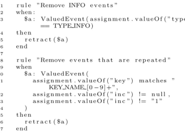
Figure 7 shows two concrete rules applied on Michelin sys-tems. These two rules are written with the Drools1
formal-ism. Drools is a rule-based expert system where knowledge bases are expressed with Java objects. The first rule removes valued events including the INFO parameter which do not contain any business value. The second rule removes valued events extracted from very specific events, i.e. those whose key matches a pattern and having a inc value that is not equal to 1. This rule, given by a Michelin expert, removes some duplicate events.
From this filtered valued event base, we reconstruct the cor-responding traces from the trace identifier pid, present in each valued event, and timestamps. We call the resulting trace set T races(Sua):
1
http://www.drools.org/
Definition 4 (T races(Sua)) Given a system under analy-sis Sua, T races(Sua) denotes its formatted trace set. T races(Sua) includes traces of the form (a1, α1)....(an, αn)
such that (ai, αi)(1≤i≤n) are (ordered) valued events having
the same identifier assignment.
We can now state that a STS model S is said exact iff. T races(S) ⊆ T races(Sua).
Algorithm 1: Trace segmentation algorithm
input : T races(Sua), optionally entry point number N and/or exit point number M
output: ST = {ST1, ..., STn}
1 Step 1. T races(Sua) segmentation
2 foreach t = (a1, α1)...(an, αn) ∈ T races(Sua) do
3 Rinit((point := val) ⊂ α1) + +;
4 Rf inal((point := val2) ⊂ αn) + +;
5 P OIN Tinit= {(point := val) | Rinit((point := val)) >
10% or belongs to the N highest ratios};
6 P OIN Tf inal= {(point := val) | Rf inal((point := val)) >
10% or belongs to the M highest ratios};
7 foreach αi= (point := val) ∈ P OIN Tinit do
8 STi= {a1(α1)...an(αn) ∈ T races(Sua) | αi⊂
α1, ∃(point := val2) ⊂ αn, (point := val2) ∈
P OIN Tf inal};
9 ST := {ST1, ..., STN};
10 Step 2. trace filtering
11 foreach t = σ1p...pσn∈ ST do
12 if ∃t0= σ01p0σ0n∈ ST such that p ∼(pid)p0,
σ1 ∼(pid)σ01, σn∼(pid)σn0 then
13 ST := ST /{t};
4.3
Trace segmentation and filtering
This module performs two steps which are summarised in Algorithm 1. It starts by splitting T races(Sua) into several trace sets STi, one for each entry point of the system Sua,
and then removes incomplete traces. Since we want a frame-work as flexible as possible, we chose to perform a statistical analysis on T races(Sua) aiming at automatically detecting the entry and exit points. This analysis is performed on the assignments (point := val) found in the first and last valued events of the traces of T races(Sua) since point captures the product physical location and especially the entry and exit points of Sua. We obtain two ratios Rinit(point := val) and Rf inal(point := val). Based on these ratios, one can deduce the entry point set P OIN Tinit and the exit point
set P OIN Tf inalif T races(Sua) is large enough.
Pragmati-cally, we observed that the traces collected during one or two days are not sufficient because they do not provide enough differences between the ratios. In this case, we assume that the number of entry and exit points, N and M , are given and we keep the first N and M ratios only. On the other hand, a week seems to offer good results. We chose to set a fixed yet configurable minimum limit to 10%. Assigne-ments (point := val) having a ratio below this limit are not retained. Then, for each assignment αi = (point := val)
in P OIN Tinit, we construct a trace set STi such that a
trace of STi has a first valued event including the
assign-ment αi, and ends with a valued event including an
assign-ment (point := val2) in P OIN Tf inal. We obtain the set
ST = {ST1, ..., STN} with N the number of entry points of
the system Sua.
Thereafter, Autofunk scans the traces in ST and tries to de-tect repetitive patterns p, ..., p. If it finds a trace t having a repetitive pattern p and another equivalent trace including this pattern p once, then t is removed since we suppose that t does not express a new and interesting behaviour. Here, traces are removed rather than deleting the repetitive pat-terns to prevent from modifying traces and to keep the trace inclusion property between the sets STi and T races(Sua).
In Algorithm 1, two traces t = σ1p, ..., pσnand t0 = σ1p0σn
are said equivalent if the patterns p, p0and the sub-sequences are equivalent, denoted with the ∼(pid)notation. Intuitively,
this relation means that the two equivalent sequences must have the same successive valued events after having removed the assignments of the variable pid.
We obtain a set ST = {ST1, ..., STN} according to the
fol-lowing proposition:
Proposition 5 Let ST =S
1≤i≤NSTi be the trace set
ob-tained from Sua. We have T races(STi) ⊆ T races(Sua).
4.4
STS generation
Given a trace set STi ∈ ST , the STS generation is
incre-mentally done by transforming traces into runs, and runs into STSs. The translation of STi into a run set denoted
Runsi is done by completing traces with states. Each run
starts by the same initial state (l0, v∅) with v∅ the empty
assignment. Then, new states are injected after each event. Runsiis formally given by the following definition:
Definition 6 (Structured Runs) Let STi be a trace set
obtained from Sua. We denote Runsithe set of runs derived
from STiwith the following inference rule:
σk(1≤k≤n)=(a1,α1)...(an,αn)∈STi
(l0,v∅)(a1,α1)(lk1,v∅)...(lkn−1,v∅)(an,αn)(lkn,v∅)∈Runsi
The above definition preserves trace inclusion between Runsi
and T races(Sua), and we can deduce the following propo-sition:
Proposition 7 Let STi be a trace set obtained from Sua.
We have T races(Runsi) ⊆ T races(Sua).
The runs of Runsi have states that are unique except for
the initial state (l0, v∅). We defined such a set to ease the
process of building a STS having a tree structure. Runs are transformed into STS paths that are assembled together by means of a disjoint union. The resulting STS forms a tree compound of branches starting from the location l0.
Parameters and guards are extracted from the assignments found in valued events:
Definition 8 Given a run set Runsi,Si=< LSi, l0Si, VSi,
V 0Si, ISi, ΛSi, →Si> is the STS expressing the behaviours
found in Runsi such that:
• LSi = {li| ∃r ∈ Runsi, (li, v∅) is a state found in r},
• l0Si = l0 is the initial location such that ∀r ∈ Runsi,
r starts with (l0, v∅),
• VSi= ∅, V 0Si= v∅,
• →Siand ΛSi are defined by the following inference rule
applied on every element r ∈ Runsi:
(li,v∅)(ai,αi)(li+1,v∅)∈r,p={x|(x:=v)∈αi},Gi= ^ (x:=v)∈αi x == v li ai(p),Gi,idV −−−−−−−−→Sili+1
Now, we have a first STS that has a tree form, describing all behaviours of the system under analysis.
Figure 4 illustrates the STSS1 obtained from the
produc-tion events of Figure 2. We have STS acproduc-tions and each one owns a parameter list. Transitions are labelled with guards derived from parameter assignments. This STS expresses the behaviours found in T races(Sua) but in a slightly dif-ferent manner. More generally, trace inclusion between an inferred STS and T races(Sua) is captured by the following proposition:
Proposition 9 Let Sua be a system under analysis and T races(Sua) be its trace set. Si is an inferred STS from
T races(Sua).
We have T races(Si) = T races(STi) ⊆ T races(Sua).
4.5
STS reduction
A STSSiis most likely too large for being analysed in an
ef-ficient manner. Given that a production system has a finite number of elements and that there should only be determin-istic decisions, the STSSishould contain branches capturing
the same sequences of events (without necessarily the same parameter assignments). Consequently, it sounds natural to try to reduce the STS obtained from the previous step. Because our goal is to produce exact models quickly, we propose to apply a lightweight STS reduction method which also aims at gathering data in order to ease the data anal-ysis later on. Our method merges complete branches that have the same action sequences whereas guards, which cap-ture parameter assignments, are merged into matrices. More precisely, a sequence of successive guards found in a branch is stored into a matrix column. By doing this, we reduce the model size and we can still retrieve original behaviours and only these ones. We still preserve trace inclusion between the reduced STS and T races(Sua).
Given a STS Si, every STS branch is initially adapted to
express sequences of guards in a vector form to ease the STS reduction. Later, the concatenation of these vectors shall give birth to matrices. This adaptation is obtained with the definition of the STS operator M at:
Definition 10 LetSi=< LSi, l0Si, VSi, V 0Si, ISi, ΛSi, →Si>
be a STS. We denote M at(Si) the STS operator which
con-sists in expressing guards of STS branches in a vector form. M at(Si) =< LM at(Si), l0M at(Si), VM at(Si), V 0M at(Si), IM at(Si)
, ΛM at(Si), →M at(Si)> where:
• LM at(Si)= LSi, l0M at(Si)= l0Si, IM at(Si)= ISi,
ΛM at(Si)= ΛSi,
• VM at(Si), V 0M at(Si)and →M at(Si) are given by the
fol-lowing rule: bi=l0 (a1(p1),G1,A1)...(an(pn),Gn,An) =====================⇒ln V 0M at(Si):= V 0M at(Si)∧ Mi= [G1, ..., Gn] l0M at(Si)
(a1(p1),Mi[1],idV)...(an(pn),Mi[n],idV)
==========================⇒→M at(Si) ln
Given a branch bi∈ (→M at(Si))
n, we also denote M at(b i) =
M the vector used with bi.
Now, we are ready to merge the STS branches that have the same sequences of actions. This last sentence can be interpreted as an equivalence relation over STS branches from which we can derive equivalence classes:
Definition 11 (STS branch equivalence class) LetSi
=< LSi, l0Si, VSi, V 0Si, ISi, ΛSi, →Si> be a STS obtained from T races(Sua) (and having a tree structure). [b] denotes the equivalence class ofSibranches such that:
[b] = {bj = l0Si (a1(p1),G1j,A1j)...(an(pn),Gnj,Anj) ========================⇒ lnj(j ≥ 1) | b = l0Si (a1(p1),G1,A1)...(an(pn),Gn,An) =====================⇒ ln}
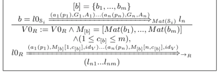
The reduced STS denoted R(Si) ofSiis obtained by
concate-nating all the branches of each equivalence class [b] found in M at(Si) into one branch. The vectors found in the branches
of [b] are concatenated as well into the same unique matrix M[b]. A column of this matrix represents a complete and
ordered sequence of guards found in one initial branch ofSi.
R(Si) is defined as follow:
Definition 12 LetSi=< LSi, l0Si, VSi, V 0Si, ISi, ΛSi, →Si>
be a STS inferred from a structured trace set T races(Sua). The reduction ofSiis modelled by the STS R(Si) =< LR, l0R,
VR, V 0R, IR, ΛR, →R> where: [b] = {b1, ..., bm} b = l0Si (a1(p1),G1,A1)...(an(pn),Gn,An) =====================⇒M at(Si)ln V 0R:= V 0R∧ M[b]= [M at(b1), ..., M at(bm)] ∧(1 ≤ c[b]≤ m), l0R
(a1(p1),M[b][1,c[b]],idV)...(an(pn),M[b][n,c[b]],idV)
=================================⇒→R
(ln1...lnm)
The resulting model R(Si) is a STS composed of variables
assigned to matrices whose values are used as guards. A matrix column represents a successive list of guards found
in a branch of the initial STSSi. The choice of the column
in a matrix depends on a new variable c[b].
Figure 4 has two branches that can be combined since they have the same action sequences. During the construction of the reduced STS depicted in Figure 6, the guards are placed into two vectors M 1 = [G1 G2] and M 2 = [G3 G3]. These are combined into the same matrix M[b]. The variable c[b]
is used to take either the guards of the first column or the guards of the second one.
The STS R(Si) has less branches but still expresses the
ini-tial behaviours described by the STS Si. This is captured
with the following proposition:
Proposition 13 Let Sua be a system under analysis and T races(Sua) be its traces set. R(Si) is a STS derived from
T races(Sua). We have T races(R(Si)) = T races(STi) ⊆
T races(Sua).
4.6
STS abstraction
Given the trace set STi∈ ST , the generated STS R(Si) can
be used for analysis purpose but is still difficult to manu-ally interpret, even for experts. This Autofunk module aims to analyse R(Si) to produce a new STS S
↑
i whose level of
abstraction is lifted by using more intelligible actions. This process is performed with inference rules, which encode the knowledge of the expert of the system. These are triggered on the transitions of R(Si) to deduce new transitions. We
consider two types of rules:
• the rules replacing some transitions by more compre-hensive ones. These rules are of the form: When Transition l1 a(p),G,A −−−−−−→R(Si)l2, condition on a(p), G, A, Then add l1 a0(p0),G0,A0 −−−−−−−−→S↑ i l2and retract l1 a(p),G,A −−−−−−→R(Si) l2.
• the rules that aggregate some successive transitions to a single transition compound of a more abstract ac-tion. These rules are of the form When Transition l1
(a1,G1,A1),...(an,Gn,An)
================⇒ ln, condition on
(a1, G1, A1), ...(an, Gn, An), Then add l1
a(p),G,A −−−−−−→S↑ i ln, and retract l1 (a1,G1,A1),...(an,Gn,An) ================⇒ ln.
The generated STSs represent recorded scenarios modelled at a higher level of abstraction. These can be particularly useful for generating documentation or better understanding how the system behaves, especially when issues are experi-enced in production. However, it is manifest that the trace inclusion property is lost with the STSs constructed by this module since sequences are modified.
If we take back our example, the actions of the STS of Fig-ure 5 are replaced with the rules of FigFig-ure 8 which change the labels 17011 and 17021 to more intelligible ones. The third rule of Figure 9 aggregates the two transitions into a unique transition indicating the movement of a product in its production line. These rules are also written using the Drools formalism. Here, T ransition are facts modelling
1 r u l e ”Mark d e s t i n a t i o n r e q u e s t s ” 2 when : 3 $ t : T r a n s i t i o n ( name m a t c h e s ”1 7 0 1 1 ”) 4 t h e n 5 $ t . c h a n g e A c t i o n ( ” D e s t i n a t i o n R e q u e s t ”) 6 end 7 8 r u l e ”Mark d e s t i n a t i o n r e s p o n s e s ” 9 when : 10 $ t : T r a n s i t i o n ( name m a t c h e s ”1 7 0 2 1 ”) 11 t h e n 12 $ t . c h a n g e A c t i o n ( ” D e s t i n a t i o n R e s p o n s e ”) 13 end
Figure 8: Two rules adding value to existing transitions
1 r u l e ” A g g r e g a t e d e s t i n a t i o n r e q u e s t s / r e s p o n s e s ” 2 when 3 $ t 1 : T r a n s i t i o n ( a c t i o n == ” D e s t i n a t i o n R e q u e s t ” , $ l f i n a l := L f i n a l ) 4 $ t 2 : T r a n s i t i o n ( a c t i o n == ” D e s t i n a t i o n R e s p o n s e ” , L i n i t == $ l f i n a l ) 5 t h e n
6 i n s e r t ( new T r a n s i t i o n ( ” P r o d u c t Advance ” , Guard ( $ t 1 . Guard , $ t 2 . Guard ) , A s s i g n ( $ t 1 . A s s i g n , $ t 2 . A s s i g n ) , $ t 1 . L i n i t , $ t 2 . L f i n a l ) ) 7 r e t r a c t ( $ t 1 )
8 r e t r a c t ( $ t 2 ) 9 end
Figure 9: STS transition aggregation rule
STS transitions. From 5 initial production events that are not self-explanatory, we generate a simpler STS constituted of one transition, clearly expressing a part of the functioning of the system.
5.
IMPLEMENTATION AND
EXPERIMEN-TATION
In this section, we briefly describe the implementation of our model inference framework for Michelin. Then, we give an evaluation on a real production system.
5.1
Implementation
Our framework Autofunk is developed in Java and mainly based on Drools 2, a Java rule-based expert system engine. Drools supports knowledge bases with facts given as Java objects. In our context, we have several bases of facts used throughout the different Autofunk modules: Events, Trace sets STi, Runs, Transitions and STSs. We chose to target
performance and simplicity while implementing Autofunk. That is why most of the steps are implemented with parallel algorithms (except the production event parsing) which are based upon the inference rules given in Section 4.
The input trace collection is constructed with a classical parser with returns Event Java objects. By now, we are not able to parallelise this part because of an issue we faced with Michelin’s logging system. The resulting drawback is that the time to parse traces is longer than expected and heavily depends on the size of data to parse. The Event base is then filtered with Drools inference rules as presented in Section 4.2. Then, we call a straightforward algorithm for reconstructing traces: it iterates over the Event base
2
http://www.drools.org/
and creates a set for each assignment of the identifier pid. These sets are sorted to construct traces given as T race Java objects. These objects correspond to T races(Sua). The generation of the trace subsets ST = {ST1, ..., STN}
and of the first STSs are done with Drools inference rules as described in Section 4, but applied in parallel. The STS reduction, and specifically the generation of STS branches equivalence classes, has been implemented with a specific algorithm for better performance. Indeed, comparing every action in STS branches in order to aggregate them is time consuming. Given a STSS, this algorithm generates a sig-nature for each branch b, i.e. a hash (SHA1 algorithm) of the concatenation of the signatures of the actions of b. The branches which have the same signature are gathered to-gether and establish branch equivalence classes (as described in Section 4.5). Thereafter, the reduced R(S) is constructed thanks to the inference rule given in Section 4.5.
5.2
Evaluation
We conducted several experiments with real sets of produc-tion events, recorded in one of Michelin’s factories at dif-ferent periods of time. We executed our implementation on a Linux (Debian) machine with 12 Intel(R) Xeon(R) CPU X5660 @ 2.8GHz and 64GB RAM.
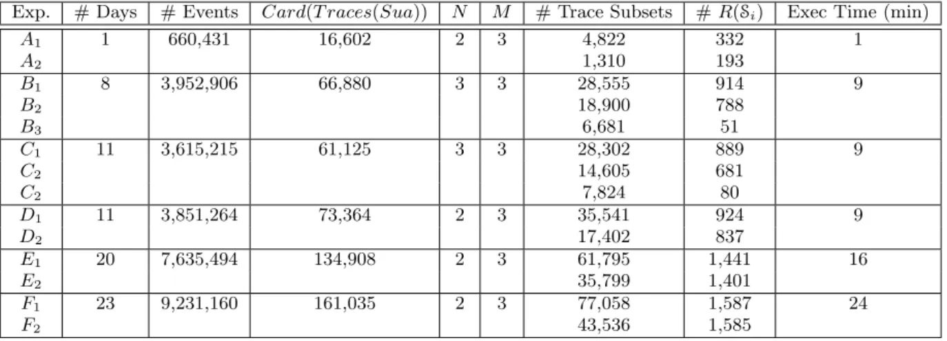
We present here the results of 6 experiments on the same production system with different event sets collected during 1, 8, 11, 20, and 23 days. These results are depicted in Figure 10. For confidentiality reasons, we are not able to provide results related to the generation of more abstract models. The third column gives the number of production events recorded on the system. The next column shows the trace number obtained after the parsing step. N and M represent the entry and exit points automatically computed with the statistical analysis. The column Trace Subsets shows how T races(Sua) is segmented into subsets {ST1, ..., STN} and
the number of traces included in each subset. These num-bers of traces also correspond to the numnum-bers of branches generated in the STSs S1, ...,SN. The eighth column, #
R(Si), represents the number of branches found in each
re-duced STSs R(S1), ..., R(SN). Finally, execution times are
rounded and expressed in minutes in the last column. First, these results show that our framework can take mil-lions of production events and still builds models quickly (less than half an hour). With sets collected during one day up to one week (experiments A, B, C, and D), models are inferred in less than 10 minutes. Hence, Autofunk can be used to quickly infer models for analysis purpose or to help diagnose faults in a system. Experiment F handled al-most 10 million events in less than half an hour to build two models including around 1,600 branches. As mentioned in Section 5.1, the parsing process is not parallelized yet, and it took up to 20 minutes to open and parse around 1,000 files (number of Michelin log files for this experiment). This is an issue we want to tackle in the next version of Autofunk. The graph shown in Figure 13 summarises the performances of our framework and how fast it is at transforming production events into models (experiments B, C and D run in about 9 minutes). It also demonstrates that doubling the event set does not involve doubling its execution time. The exponen-tial trend line reveals that the overall framework scales well, even with the current parsing implementation.
Exp. # Days # Events Card(T races(Sua)) N M # Trace Subsets # R(Si) Exec Time (min) A1 1 660,431 16,602 2 3 4,822 332 1 A2 1,310 193 B1 8 3,952,906 66,880 3 3 28,555 914 9 B2 18,900 788 B3 6,681 51 C1 11 3,615,215 61,125 3 3 28,302 889 9 C2 14,605 681 C2 7,824 80 D1 11 3,851,264 73,364 2 3 35,541 924 9 D2 17,402 837 E1 20 7,635,494 134,908 2 3 61,795 1,441 16 E2 35,799 1,401 F1 23 9,231,160 161,035 2 3 77,058 1,587 24 F2 43,536 1,585
Figure 10: Results of 6 experiments on a Michelin industrial system
In Figure 10, the difference between the number of trace subsets (7th column) and the number of branches included in the STSs R(Si) (8th column) clearly shows that our STS
reduction approach is effective. For instance, with experi-ment B, we reduce the STSs by 91.88% against the initial trace set T races(Sua). In other words, 91% of the original behaviours are packed into matrices.
We also extracted the values of columns 4 and 7 in Figure 10 to depict the stacked bar chart illustrated in Figure 11. This chart shows, for each experiment, the proportion of complete traces kept by Autofunk to build models, over the initial number of traces in T races(Sua). Autofunk has kept only 37% of the initial traces in Experiment A because its initial trace set is too small and contains many incomplete behaviours. During a day, most of the recorded traces do not start or end at entry or exit points, but rather start or end somewhere in production lines. Indeed, a workshop contains storage areas where products can stay for a while, depending on the production campaigns or needs for instance. That is why, on a single day, we can find so many incomplete traces. With more production events, such a phenomenon is limited because we absorb these storage delays.
We can also notice that experiments C and D have simi-lar initial trace sets but experiment C owns more complete traces than experiment D by 12%, which is significant. Fur-thermore, experiments B and C take 3 entry points into ac-count while the others only take 2 of them. This is related to the fixed limit of 10% we chose to ensure truly entry points to be automatically selected. The workshop we analysed has three entry points whose two are mainly used. The third entry point is employed to equilibrate the production load between this workshop and a second one located close to it in the same factory. Depending on the period, this entry point may be more or less sollicitated, hence the difference between experiments B, C and experiment D. Increasing the limit of 10% to a higher value would change the value of N for experiments B and C, but would also impact ex-periment A by introducing false results since incorrect entry points could be selected. By means of a manual analysis, we concluded that 10% was the best ratio for removing incom-plete traces in our experiments. 30% of initial traces have been removed, which is close to the reality. However, this
Figure 11: Proportions of complete traces
simple analysis could be improved in the future.
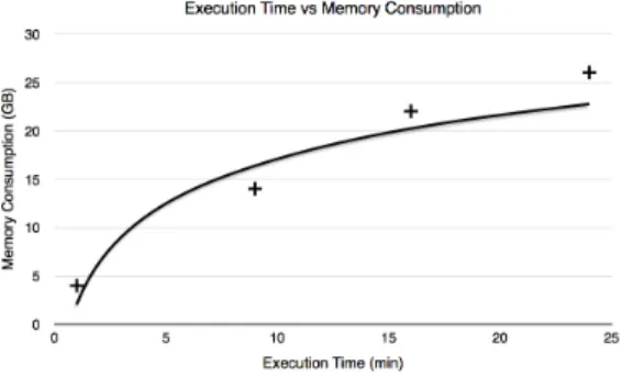
Another potential issue with our parsing implementation is that every event has to be loaded in memory, so that we can perform computation and apply our algorithms on them. However working with millions of Java objects re-quires enough memory, i.e. memory consumption depends on the amount of initial traces. We compared execution time and memory consumption in Figure 12, showing that memory consumption tends to follow a logarithmic trend. In the next version of Autofunk, we plan to work on im-proving memory consumption even if it has been considered acceptable as is by Michelin.
6.
CONCLUSION
This paper presents Autofunk, a fast and scalable framework combining model inference and expert systems to generate models from production systems. Given a large set of pro-duction events, our framework infers exacts models whose traces are included in the initial trace set of a system un-der analysis. We chose to design Autofunk for targeting high performance. Our evaluation shows that this approach is suitable in the context of production systems since we quickly obtain STS trees reduced by 90% against the
origi-Figure 12: Memory consumption vs execution time
Figure 13: Execution time vs events
nal trace sets of the system under analysis.
Nevertheless, many aspects need to be investigated and proved in the future. From a technical perspective, our im-plementation should be enhanced to speed up the event pars-ing, for instance by considering a message queuing protocol, and to optimize memory consumption. Our STS reduction approach could also be improved by concatenating partial equivalent STS branches. However, a naive solution would affect performance as partial branch concatenation is time consuming, and we do not want to sacrifice execution speed. We also plan to use this framework to propose a new test-ing approach taktest-ing advantage of the inferred models. In short, inferred models could be used to generate event-based scenarios to test production systems, and an improved ver-sion of Autofunk could check the compliance of the recorded event sets against inferred models.
7.
REFERENCES
[1] P. A. Abdulla, L. Kaati, and J. Hogberg. Bisimulation minimization of tree automata. Technical report, In Proc. 11th Int. Conf. Implementation and Application of Automata, volume 4094 of LNCS, 2006.
[2] D. Amalfitano, A. R. Fasolino, P. Tramontana, B. D. Ta, and A. M. Memon. Mobiguitar – a tool for automated model-based testing of mobile apps. IEEE Software, NN(N):NN–NN, 2014.
[3] S. Anand, M. Naik, M. J. Harrold, and H. Yang. Automated concolic testing of smartphone apps. In Proceedings of the ACM SIGSOFT 20th International Symposium on the Foundations of Software
Engineering, FSE ’12, pages 59:1–59:11, New York,
NY, USA, 2012. ACM.
[4] D. Angluin. Learning regular sets from queries and counterexamples. Information and Computation, 75(2):87 – 106, 1987.
[5] S. Artzi, A. Kiezun, J. Dolby, F. Tip, D. Dig, A. Paradkar, and M. Ernst. Finding bugs in web applications using dynamic test generation and explicit-state model checking. Software Engineering, IEEE Transactions on, 36(4):474–494, 2010.
[6] W. Choi, G. Necula, and K. Sen. Guided gui testing of android apps with minimal restart and approximate learning. In Proceedings of the 2013 ACM SIGPLAN International Conference on Object Oriented
Programming Systems Languages & Applications, OOPSLA ’13, pages 623–640, New York, NY, USA, 2013. ACM.
[7] L. Frantzen, J. Tretmans, and T. Willemse. Test Generation Based on Symbolic Specifications. In J. Grabowski and B. Nielsen, editors, FATES 2004, number 3395 in Lecture Notes in Computer Science, pages 1–15. Springer, 2005.
[8] H. Hungar, T. Margaria, and B. Steffen. Model generation for legacy systems. In M. Wirsing, A. Knapp, and S. Balsamo, editors, Radical
Innovations of Software and Systems Engineering in the Future, 9th International Workshop, RISSEF 2002, Venice, Italy, October 7-11, 2002, Revised Papers, volume 2941 of Lecture Notes in Computer Science, pages 167–183. Springer, 2002.
[9] A. Memon, I. Banerjee, and A. Nagarajan. Gui ripping: Reverse engineering of graphical user interfaces for testing. In Proceedings of the 10th Working Conference on Reverse Engineering, WCRE ’03, pages 260–, Washington, DC, USA, 2003. IEEE Computer Society.
[10] A. Mesbah, A. van Deursen, and S. Lenselink. Crawling Ajax-based web applications through dynamic analysis of user interface state changes. ACM Transactions on the Web (TWEB), 6(1):3:1–3:30, 2012.
[11] M. Pradel and T. R. Gross. Automatic generation of object usage specifications from large method traces. In Proceedings of the 2009 IEEE/ACM International Conference on Automated Software Engineering, ASE ’09, pages 371–382, Washington, DC, USA, 2009. IEEE Computer Society.
[12] M. Salah, T. Denton, S. Mancoridis, and A. Shokouf. Scenariographer: A tool for reverse engineering class usage scenarios from method invocation sequences. In In ICSM, pages 155–164. IEEE Computer Society, 2005.
[13] H. Zhong, L. Zhang, T. Xie, and H. Mei. Inferring specifications for resources from natural language api documentation. Autom. Softw. Eng., 18(3-4):227–261, 2011.