HAL Id: ujm-00297147
https://hal-ujm.archives-ouvertes.fr/ujm-00297147
Submitted on 6 Feb 2009
HAL is a multi-disciplinary open access archive for the deposit and dissemination of sci-entific research documents, whether they are pub-lished or not. The documents may come from teaching and research institutions in France or abroad, or from public or private research centers.
L’archive ouverte pluridisciplinaire HAL, est destinée au dépôt et à la diffusion de documents scientifiques de niveau recherche, publiés ou non, émanant des établissements d’enseignement et de recherche français ou étrangers, des laboratoires publics ou privés.
problem-based algorithm for digital inline holography
Jérôme Gire, Christophe Ducottet, Loïc Denis, Éric Thiébaut, Ferréol Soulez
To cite this version:
Jérôme Gire, Christophe Ducottet, Loïc Denis, Éric Thiébaut, Ferréol Soulez. Signal to noise charac-terization of an inverse problem-based algorithm for digital inline holography. ISFV13, 13th Interna-tional Symposium on Flow Visualization, Jul 2008, Nice, France. pp.Session 39, ID226. �ujm-00297147�
Signal to noise characterization of an inverse
problem-based algorithm for digital in-line holography
J Gire1,2,4, C Ducottet1,4, L Denis1,3, E Thiébaut2, F Soulez1,21Laboratoire Hubert Curien (ex-LTSI) ; CNRS, UMR5516 ; Université Jean Monnet;
18 rue Pr Benoît Lauras, F-42000 Saint-Etienne, France
2Université de Lyon, Lyon, F-69000, France ; Université Lyon 1, Villeurbanne, F-69622, France ;
Centre de Recherche Astronomique de Lyon, Observatoire de Lyon,
9 avenue Charles André, Saint-Genis Laval cedex, F-69561, France ; CNRS, UMR 5574 ; Ecole Normale Supérieure de Lyon, Lyon, France
4Institut Supérieur des Techniques Avancées de Saint-Etienne, Saint-Etienne, France
KEYWORDS:
Main subject(s): digital holography; in-line holography; inverse problem; signal to noise ratio;
Fluid: micro-particles, jet flows, tracking
ABSTRACT:In-line holography is a 3D imaging technique which has been used for many years, especially in experimental fluid mechanics for the 3D localization and sizing of micro-particles from the acquisition of a single 2D image (hologram). This technique is easily usable in an industrial environment thanks to its simple setup.
We have recently presented an algorithm of hologram analysis based on an “inverse problem” approach. This method find the best model which can explain the hologram and this is realized iteratively by removing at each step the contribution of the detected particle. This method can overcome some limitations of classical approach: like the enlargement of the accessible studied field.
Nevertheless, some questions remain on the limitations of the method. We propose in this paper an analysis of the evolution of the signal to noise ratio to clarify the limitations like the size of the studied field, the effect of the cleaning of already detected particles during the process and the influence of the noise generated by the other particles.
1 Introduction
In-line holography is a 3D imaging technique which has been used during many years, especially in experimental fluid mechanics [1, 2]. In particular, to return the 3D localization and sizing of small objects from the acquisition of a single 2D image (hologram). The digital version of this technique uses a direct recording on a sensor and a digital processing of holograms without any optical reconstruction [3, 4]. Thanks to the simple experimental setup and the easy operating, the technique is usable in a real industrial environment.
Numerous techniques have been developed to analyze micro-particle holograms [3, 4]. They are mostly based on digital reconstruction by the simulation of hologram diffraction. These methods are often limited to low concentrated holograms due to the intrinsic speckle noise which is a major problem in in-line holography [5, 6]. Some techniques have been developed to reduce it, like off-axis or in-line recording and off-axis viewing technique [7, 8, 9, 10, 11]. These techniques overcome some problems like speckle noise but require a more complex setup.
We recently proposed a new approach for the hologram processing [12, 13]. This approach, based on an “inverse problem” formulation, consists in searching for the parameters of localization and size of each particle by minimizing the difference between the recorded hologram and the model of this hologram. This minimization is made iteratively by looking for, at each iteration, the parameters of the most likely particle and then subtracting the contribution of this particle from the initial data (cleaning). The parameters of the particle are determined in two steps: an extensive search over a given sampling of the parameter space, followed by a local refinement step performed by non-linear optimization.
This approach was tested on both synthetic and real holograms. The obtained results showed an improvement of the accuracy of the particles localization and an increase in the accessible field of view beyond the size of the sensor. A study of some benefits of this approach have already been realized [14].
Nevertheless, a lot of questions about this algorithm had not yet been studied. In particular: • the limit size of the studied field
• the benefit of the cleaning step[14]
• the influence of the noise and of the other particles during the optimization step • the influence of experimental parameters.
The present article proposes a detailed study of the behavior of the algorithm. For that purpose, we define a signal to noise ratio (SNR) adapted to the algorithm and we propose a study of its evolution during iterations of the algorithm for different levels of background noise.
In section 2 we recall the principle of the processing algorithm based on an “inverse problem” approach. Then we propose, in section 3, a definition of the signal to noise ratio for this approach and describe the method to calculate it. Then we study, in section 4 the evolution of the SNR and finally we describe, in section 5 the behavior of the algorithm.
2 Principle of the algorithm based on inverse problem
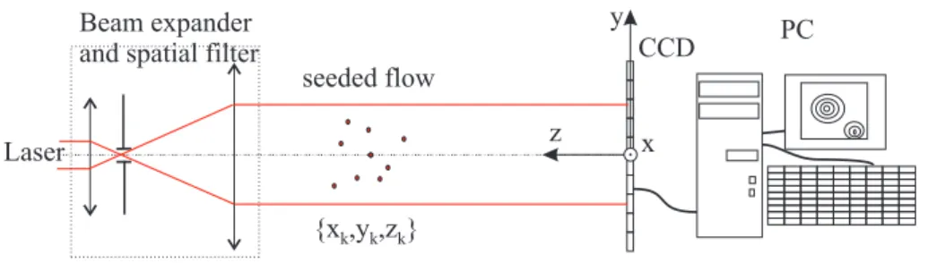
In that study, we consider digital holograms of a set of spherical particles recorded in the in-line holography configuration (Gabor setup) (figure 1). We address the problem of recovering the position and size of all the recorded particles from a given digital hologram.
The principle of the approach we propose in [12] is to consider this problem as an “inverse prob-lem”. The associated direct problem is the computation of the intensity function in the hologram plane given the position and size of all the particles. This latter problem, known as the recording
model determination, is well known and particularly simple in the context of Fresnel’s diffraction approximation. We then propose to solve the “inverse problem” by minimizing the difference be-tween the recorded hologram and the model of this hologram. This minimization is made iteratively by looking for, at each iteration, the parameters of the most likely particle and then subtracting the contribution of this particle from the initial data (cleaning).
This section recalls briefly the recording model, the “inverse problem” formulation and its iterative resolution. A more detailed presentation can be found in [12, 13].
2.1 Recording model of the hologram
PC
Laser
CCD Beam expander
and spatial filter
z y
x seeded flow
{x ,y ,z }k k k
Figure 1: The in-line holography setup
We consider an in-line holographic setup (see figure 1) where studied particles are illuminated by the laser beam and both reference wave and object wave interfere and are recorded by the detector (typically a CCD sensor). The resulting hologram expression is a sum of terms depending on the location and size of each particle. In the case of digital holography of spherical micro-particles, each particle is described by few parameters{xk, yk, zk, rk}: x, y, z represent the spatial coordinates and r
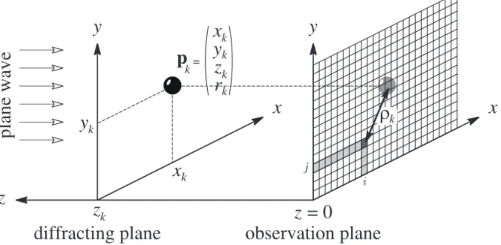
the radius. The notations and coordinate system we use are summarized in figure 2. The simplified expression of hologram intensity measured by the detector can be written as follows [13]:
I(x, y) = I0−
n
∑
k=1
αkgk(x − xk, y− yk) + Ibg(x, y) (1)
whereαkis an amplitude factor of the diffraction pattern of the k-th particle, I0represents the incident
intensity on the sensor and Ibg the background noise. The function gk(x, y) represents the diffraction pattern of one particle and is given by the following equation:
gk(x, y) = πr2k λzk J1c à 2πrk p x2+ y2 λzk ! sin µπ(x2+ y2) λzk ¶ (2) whereλis the laser wavelength. Let us notice that the speckle noise due to second order interference terms is negligible compared to the amplitude of the diffraction patterns of the other particles (Meng [5]). We therefore neglect this noise. The background noise (Ibg(x, y)) comprises the noise due to
experimental setup, due to the electronic noise and due to the quantization noise.
The detector is a matrix of size (Ni,Nj), thus the intensity is only known on discrete values (i, j).
The recorded data (1) on the pixel[i, j] are:
d[i, j] = I0−
n
∑
k=1
αkgk[i, j] + Ibg[i, j] (3)
where gk[i, j] = gk(x − xk, y− yk) with x − xk= i∆ξand y− yk= j∆ξ.
This recording model of a hologram is an additive model: the hologram intensity consists of the sum of the diffraction-patterns of the n particles plus a remaining background noise Ibg.
Figure 2: Notations used in the hologram model.
2.2 Inverse problem formulation
The experimental digital hologram is given as a matrix of data d[i, j]. The inverse problem consists in finding the value I0,{αk}k=1,...n and the set of parameters of the particles{xk, yk, zk, rk}k=1,...nwhich best model this hologram.
We denotes m[i, j] the parametric model of the hologram defined as:
m[i, j] = I0−
n
∑
k=1
αkgk[i, j] (4)
The latter inverse problem can be expressed as a global optimization problem. It consists in finding the optimal set of parameters which minimizes the penalty function
P
of weighted least squares defined by:P
=∑
w (m[i, j] − d[i, j])2 (5) The operator∑
wrepresents a weighted sum over the matrix of pixels(Ni, Nj). For any matrix a[i, j],
it is defined as:
∑
w a[i, j] = Ni∑
i=1 Nj∑
j=1 w[i, j] a[i, j]. (6)where w[i, j] is a weight matrix taking into account the truncation effect and possible dead pixels and can be defined as:
w[i, j] = ½
1 if the pixel (i, j) is measured,
0 otherwise. (7)
2.3 Iterative particle detection
We have proposed an iterative algorithm to solve this problem particle per particle by a local opti-mization [12].
At iteration ℓ, the parameters{xℓ, yℓ, zℓ, rℓ} of the ℓ-th particle are determined by minimization of the weighted least-squares penalty function
P
ℓ:P
ℓ=∑
w
(mℓ[i, j] − dℓ[i, j])2 (8) where mℓ[i, j] is the intensity contribution of the ℓ-th particle and dℓ[i, j] is the centered residual data at the ℓ-th step.
mℓ[i, j], which can be considered as the model of the ℓ-th particle, is given by:
mℓ[i, j] = Iℓ−αℓgℓ[i, j] (9) with Iℓthe incident intensity on the residual hologram.
dℓ[i, j] represents the residual centered hologram after removing the contribution of the ℓ − 1 first particles. It can be detailed from equations (3) and (4) as follows:
dℓ[i, j] = d[i, j] + ℓ−1
∑
k=1
αkgk[i, j] + aℓ (10) where aℓcorresponds to the centering constant such as:
∑
w
dℓ[i, j] = 0 . (11)
If we optimize with respect to Iℓ andαℓfor other parameters fixed, it can be shown [13] that the minimization of
P
ℓis equivalent to the maximization of theQ
ℓcriterion defined by:Q
ℓ= µ∑
w dℓ[i, j] ˜gℓ[i, j] ¶2∑
w ˜ g2ℓ[i, j] (12)where ˜gℓis a centered version of gℓsuch that:
∑
w
˜
gℓ[i, j] = 0 (13)
3 Proposed definition of the signal to noise ratio
Some important questions about the previous algorithm have not yet been studied. In particular, we infer that the first iterations are delicate since few particles have been removed. In the same way we don’t know precisely what are the accurate limits for the size of the analyzed field, and for background noise or for the number of particles.
The aim of this section is to define a signal to noise ratio (SNR) adapted to the study of these questions. This ratio, defined at a given iteration of the optimization algorithm, will evaluate the relative contribution of a signal term corresponding to the optimized particle and two noise terms respectively due to the other remaining particles and due to background noise.
We first present a definition of the signal to noise ratio. Then we propose a numerical method to compute it.
3.1 Definition of the SNR
At iteration ℓ, residual data are given by equation (10) and including (3) in (10), we have:
dℓ[i, j] = I0−αℓgℓ[i, j] −
n
∑
k=ℓ+1
αkgk[i, j] + Ibg[i, j] + aℓ (14) by inserting (14) in (12), and tacking accounts of
∑
w ˜ gℓ[i, j] = 0:
Q
ℓ= 1∑
w ˜ g2ℓ[i, j] αℓ∑
w gℓ[i, j] ˜gℓ[i, j] | {z } t1 + n∑
k=l+1 αk∑
w gk[i, j] ˜gℓ[i, j] | {z } t2 +∑
w Ibg[i, j] ˜gℓ[i, j] | {z } t3 2 (15)During the optimization step, we search for parameters {x+ℓ, y+ℓ, z+ℓ, rℓ+} of the function ˜gℓwhich maximize
Q
ℓ. In this equation three components can be distinguished: (t1) the energy on the sensor ofthe ℓ-th particle, (t2) the contribution of residual particles, and (t3) the contribution of the background
noise.
To study the efficiency of the optimization, we can modeled (t2) and (t3) as two random
compo-nents: t2= n
∑
k=ℓ−1 αk∑
w Gk[i, j] ˜gℓ[i, j] (16) where Gk[i, j] is a random process defined by:Gk[i, j] = gZkRk(i∆ξ− Xk, j∆ξ−Yk) (17)
where Xk,Yk, Zk, Rkare random variables.
t3=
∑
w
Ibg[i, j] ˜gℓ[i, j] (18) where Ibg is a random process (background noise).
Then, we can define the signal to noise ratio as:
SNRℓ=
t12
var(t2+ t3)
(19) where var is the statistical variance operator.
As (t2) and (t3) are statistically independent, we have:
var(t2+ t3) = var(t2) + var(t3) (20)
Similarly, the Gkprocesses are identical and each other independent as we suppose that there isn’t
any interaction between particles. We can denote them G and we have: var(t2) = Ã n
∑
k=ℓ−1 α2 k ! var µ∑
w G[i, j] ˜gℓ[i, j] ¶ (21) =α20(n − ℓ) var µ∑
w G[i, j] ˜gℓ[i, j] ¶ (22)ifαkare identical and equal toα0.
The noise variance can also be simplified if the noise Ibg is stationary. Its expression becomes:
var(t3) = var(Ibg)
∑
w ˜ g2ℓ[i, j] (23) =σ2bg∑
w ˜ g2ℓ[i, j] (24)whereσbg is the standard deviation of the background noise.
According to equations (20), (21) and (23), the signal to noise ratio (19) becomes:
SNRℓ= α2 0 µ
∑
w ˜ g2ℓ[i, j] ¶2 α2 0(n − ℓ) var µ∑
w G ˜gℓ[i, j] ¶ +σ2bg∑
w ˜ g2ℓ[i, j] (25) 3.2 Numerical calculationIn this subsection, we consider that variance of the background noise is known and that the set of particles is uniformly distributed into a rectangular spatial domain B. We then present the numerical calculation of the value of the previous SNR for any iteration ℓ.
Given the iteration number and the parameters of the particle optimized at step ℓ, all the terms of equation 25 are easily calculable except the variance of the noise term due to the other particles defined as: var(t2′) = var µ
∑
w G[i, j] ˜gℓ[i, j] ¶ (26) 3.2.1 Cleaning effectLet us notice that the influence of the cleaning must be taken into account in the calculation of this variance. Indeed, as the particles are removed from the hologram, the statistical distribution of the remaining particles changes. More precisely, without tacking account the influence of noise, particles are removed in decreasing order of energy. In the case of mono-disperse particles, the ones of higher energy are the ones located on the optical axis, and their energy decreases with the distance (ρ) to the optical axis.
As the sensor is a square, at step ℓ, all the particles located in a square of size 2ρ have been removed. As the particles are supposed to be uniformly distributed, we approximately can link the iteration number ℓ and the distanceρto the optical axis by:
ρ2= Sℓ
4n (27)
where S is the projected surface of the volume containing the particles, and n is the number of parti-cles.
Then, at each iteration ℓ, the remaining particles are uniformly distributed over a domain Bρ defined as the initial domain B deprived of the square cylinder of size 2ρcentered on the optical axis.
From that point, the statistical variance of t2′ can be calculated as:
var(t2′) = E(t2′2) − E(t2′)2 (28)
3.2.2 Calculation of E(t2′)
As we saw in section 3.1,
G[i, j] = gR,Z(i∆ξ− X, j∆ξ−Y ) (29)
Where X ,Y, Z, R are random variables.
We suppose that these variables are independents and uniformly distributed on intervals such as: (X,Y ) ∈ B = [Xa, Xb] × [Ya,Yb] (30)
Z= [Za, Zb] (31)
R= [Ra, Rb] (32)
When particles are removed, the domain B is deprived of the square of size 2ρ. The variables X and Y are randomly distributed on Bρ= B \ square(0, 2ρ)
E(t2′) = E ·
∑
w G[i, j] ˜gℓ[i, j] ¸ (33) = Z Bρ Z Zb Za Z Rb Ra 1 Bρ 1 Zb− Za 1 Ra− Rb∑
w gz,rg˜ℓdx dy dz dr (34)∑
w gz,rg˜ℓ =∑
w gz,r(i∆ξ− xℓ, j∆ξ− yℓ) ˜gℓ(i∆ξ− xℓ, j∆ξ− yℓ) (35) =∑
w gz,r(∆ξ(i − i′),∆ξ( j − j′)) ˜gℓ(i∆ξ, j∆ξ) (36) with x = i′∆ξ (37) y = j′∆ξ (38)If we note gz,r[i, j] = gz,r(i∆ξ, j∆ξ), for i′and j′integer, we have:
∑
w
gz,rg˜ℓ = (gz,r∗ w ˜gℓ) [i′, j′] (39) where∗ is the discrete convolution product.
If we approximate the integral on x, y by a discrete sum on[i′, j′], the equation (33) becomes:
E(t2′) ≈ ∆ξ 2 I(Bρ) 1 Za− Zb 1 Ra− Rb Z Zb Za Z Rb Ra (i′, j
∑
′)∈Bρ (gz,r∗ w ˜gℓ) [i′, j′] dz dr (40) = ∆ξ 2 I(Bρ)(i′, j∑
′)∈Bρ ³ g(1)∗ w ˜gℓ ´ [i′, j′] (41) where g(1)= 1 Za− Zb 1 Ra− Rb Z Zb Za Z Rb Ra gz,rdz dr (42)3.2.3 Calculation of E(t2′2)
In the same way, we have:
E(t2′2) = ∆ξ 2 I(Bρ) 1 Za− Zb 1 Ra− Rb Z Zb Za Z Rb Ra (i′, j
∑
′)∈Bρ (gz,r∗ w ˜gℓ)2[i′, j′] dz dr (43)4 Study of the SNR evolution
In this section, we study the evolution of the SNR during iterations of the algorithm for different levels of background noise. We first define the parameters of holograms used. Then, the study is done both theoretically using the expression given in the previous section and experimentally using a set of simulated holograms. Finally, we compare the results and conclude on the validation of the theoretical study and approximations made in the calculation in section 3.2.
4.1 Parameters of the study
(a) (b)
Figure 3: (a) Example of a hologram simulation [14] (1024× 1024) made with 2000
par-ticles (radius of 50µm) spread throughout a volume of 27.44× 27.44 × 50mm located at
z0= 250mm. The pixel size is 6.7 × 6.7µm and the laser wavelength is 0.532µm. The
holo-gram is coded on 8 bits depth. (b) Illustration of the distribution of particles throughout the volume: 125 particles are located on the sensor (dark gray area of width L), 500 out-of-field particles are located on the white area (4 times the sensor area), and 1500 particles are located around the white area (in the light gray part) which corresponds to the noise.
We consider particles with constant radius r0that are randomly distributed under a uniform
prob-ability law throughout a volume centered on the optical axis and located at the distance z0. The
holo-grams (example in figure 3a) are realized with a sensor of 1024× 1024 (pixels size of 6.7 × 6.7µm) placed at about z0= 250mm from the studied volume. Figure 3b illustrates the transverse distribution
of 2000 particles (radius of 50µm) throughout the volume of 27.44× 27.44 × 50mm: 125 particles are located on the sensor (dark gray rectangle), 500 out-of-field particles are located on the white
rectangle (4 times the sensor surface), and 1500 particles are located in the light gray part. These latter particles are not detected by the algorithm (since they are outside of the explored field of view). They therefore contribute to the noise. The light gray rectangle corresponds to the projected surface of the volume (16 times the sensor surface). The laser wavelength is 0.532µm. This parameters have already been used in reference [14]. We add to this hologram a white Gaussian noise with a variance depending on a percentage of the hologram amplitude.
4.2 Theoretical study
The signal to noise ratio can be calculated theoretically according to the equation (25). For that, three components have to be calculated for different distancesρfrom the hologram center: the energy of a particle, the variance of the other particles (according to section 3.2), and the variance of the background noise. To simplify the calculation of the term corresponding to the variance of the other particles (ie equations (40) and (43)), we take the same longitudinal distance for all the particles as the mean longitudinal distance zm= 225mm. Then, using the relation in (27), the SNR can be plotted
as a function of the iteration number or of the distanceρfrom the optical axis.
On figure 4, we can see several curves of the SNR plotted for different level of background noise.
0 200 400 600 800 1000 1200 5 10 15 20 25 30 35
Distance from the center (pixels)
S NR le ve l (d B )
Signal to noise ratio
in-field out-of-field 0% 5% 10% 15% 20% 25%
Figure 4: Theoretical curves of the SNR evolution as a function of the distance to the optical
axis. The SNR is plotted for different background noise level depending on a percentage of the hologram amplitude (from 0% to 25%). The vertical dot-dash line represents the sensor border.
4.3 Numerical experimentation
In this subsection, we study the evolution of the SNR from the results of the analysis of simulated holograms for different levels of noise. For that, the components of the SNR are estimated, during the iterations of the inverse algorithm using the optimal parameters given by the algorithm.
The component t1of
Q
ℓ (15) and can be obtained from the energy of the particle. The statistical variance of the noise (components t2 and t3) is estimated by the computation of the spatial varianceof the numerator of
Q
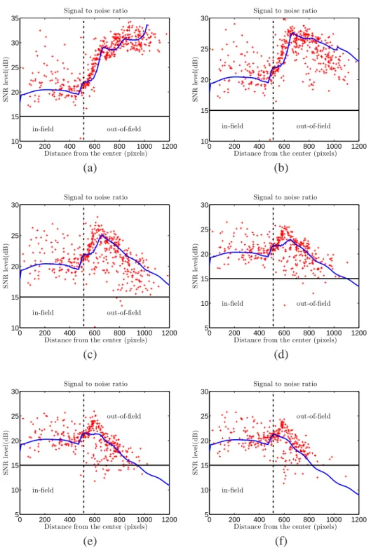
ℓ on a square ring around the hologram center with a radius corresponding to the distance ρ. On figure 5, we can see several curves of SNR for different background noise levels (white Gaussian noise). The variance of background noise corresponds to a percentage of thehologram amplitude: 0% for (5a) to 25% for (5f) with a step of 5% between each figure. Theoretical curves (see section 4.2) are plotted in blue and ones calculated on the simulated hologram in red. The vertical dot-dash line represents the sensor border. The horizontal line shows the SNR limit value (see section 5). 0 200 400 600 800 1000 1200 10 15 20 25 30 35 in-field out-of-field Signal to noise ratio
Distance from the center (pixels)
S NR le ve l( d B ) 0 200 400 600 800 1000 1200 10 15 20 25 30 in-field out-of-field Signal to noise ratio
Distance from the center (pixels)
S NR le ve l( d B ) (a) (b) 0 200 400 600 800 1000 1200 10 15 20 25 30 in-field out-of-field Signal to noise ratio
Distance from the center (pixels)
S NR le ve l( d B ) 0 200 400 600 800 1000 1200 5 10 15 20 25 30 in-field out-of-field Signal to noise ratio
Distance from the center (pixels)
S NR le ve l( d B ) (c) (d) 0 200 400 600 800 1000 1200 5 10 15 20 25 30 in-field out-of-field Signal to noise ratio
Distance from the center (pixels)
S NR le ve l( d B ) 0 200 400 600 800 1000 1200 5 10 15 20 25 30 in-field out-of-field Signal to noise ratio
Distance from the center (pixels)
S NR le ve l( d B ) (e) (f)
Figure 5: Evolution of the SNR during the detection of particles. Theoretical curves are
plotted in blue and ones calculated on simulated holograms in red (+). The evolution
is studied for several noise levels. The variance of background noise corresponds to a percentage of the hologram amplitude: 0% for (a) to 25% for (f) with a step of 5% between each figure. The vertical dot-dash line represents the sensor border. The horizontal line shows the SNR limit value (see section 5).
4.4 Comparison and validation
In this section we compare the theoretical curves (section 4.2) of the signal to noise ratio to the curves obtained by the analysis of simulated holograms (section 4.3).
When particles are on the sensor area, we can observe (figure 5) a large dispersion of the exper-imental points. When particles are located out-of-field the point are close to the theoretical curve. This dispersion at the beginning is mainly due to the detection order of particles. Indeed, at this point, particles are not detected as a function of the distanceρ. As a consequence, the variance of the noise mainly varies as a function of the local neighborhood of the particle. On the contrary, out-of-field particles are detected as a function of their distance to the optical axis and the SNR curves on the sim-ulations are in agreement with the theoretical ones. Another source of dispersion in experimentations is due to the influence of the variation of the longitudinal position z of particles. In the theoretical calculation we take this parameter constant (see section 4.2).
For the three first curves (5a and 5b), we can see that the SNR on the theoretical curves is higher than the one of the simulated hologram. It can be explained by additional sources of noise which appear during the iterations of the algorithm. For example, due to quantization errors or mismod-elling, the contribution of a given particle is not totally removed during the cleaning step. This effect increases the background noise level and decreases the SNR for the out-of-field particles.
On the whole, we can consider that the model is in good agreement with the numerical experi-mentations. Even if the theoretical model does not exactly react in the same way as the algorithm, especially for in-field particles, it is a good tool to explain the SNR evolution. It gives an average value of the evolution of the SNR for a given setup, and a given estimation of the particle density and background noise level.
5 Analysis of the algorithm behavior
In the first part of the curves (ρ< 512), the particles are in the field. The noise is dominated by the remaining particles. The SNR is quite constant (it is slightly increasing and then slightly decreasing) because the decrease in the particle energy is roughly compensated by the decrease of the noise due to cleaning. In the second part, the SNR is increasing until a maximum. The particles energy continue to decrease, but the noise due to the remaining particles is less important so as the SNR is increasing. Then the background noise becomes to be significant and limit the increasing of the SNR. In the third part, the background noise is dominant and the SNR is decreasing until the algorithm stops.
We remark that the effect of the cleaning helps us to detect out-of-field particles even far away from the hologram borders and as consequence it allows to enlarge the size of the studied field. The effect of the cleaning provides a great improvement when there is a high number of particle in the studied field. It has a lower effect when the background noise is very high compared to the noise generated by other particles or when the density of particle is low.
According to figure 5 we can roughly estimate a limit distance beyond which the algorithm does not detect particles anymore. We can then derive a limit SNR. In the case of figures 5a to 5c the detection is not limited by the background noise but only because we choose to stop the algorithm after the detection of 500 particles. For figures 5d to 5f the detection is limited by the background noise level. For these curves we can define a limit value of the SNR beyond which the particles are no longer detected. We estimate this value to 15dB by averaging the SNR value of the farthest particles from the optical axis (represented by an horizontal line on figure 5).
The previous value can help to define working limits of the algorithm. Given the setup parameters, the background noise and the number of particles, a theoretical SNR curve can be calculated. If the
SNR of particles located in the center (ρ= 0) is below the limit SNR, the starting of the algorithm may be critical: the first particles may not be correctly detected and/or estimated. If the SNR at starting is high enough, the limit size of the studied field can be estimated by finding the greatest distanceρ having a SNR greater than the limit SNR. These last statements must be verified on more detailed experimentations.
6 Conclusion
We have proposed in this contribution a signal to noise ratio study of our inverse problem approach based algorithm. This study relies on a definition of the SNR adapted to the optimization criterion. It allows the study of the evolution of the SNR during the iterations of the algorithm for different levels of noise.
We have shown that this theoretical SNR can be numerically calculated if the statistical distribu-tions of the particles parameters are given. Then, after a comparison of the theoretical results with numerical experimentations on simulated holograms, we have validated our theoretical approach.
Finally, the shape of the curves as a function of the particle distance have been analyzed for different levels of background noise. A limit SNR has been highlighted on the curves providing a way to define the working limits of the algorithm.
Future work has to be realized to confirm the precise influence of the limit SNR on real holograms. The proposed SNR definition can also be used to study the effect of experimental parameters as the hologram distance, the number of particles or the number of pixels of the sensor. It can also be noticed that the proposed approach can be adapted for the SNR study of other digital inline holography algorithms.
References
[1] Xu L, Peng X, Guo Z, Miao J, and Asundi A. Imaging analysis of digital holography. Optics Express, 13(7):2444– 2452, 2005.
[2] Kreis T M. Handbook of Holographic Interferometry, Optical and Digital Methods. Wiley-VCH, Berlin, 2005. [3] Poon T C, Yatagai T, and Jüptner W. Digital holography – Coherent optics of the 21st century: introduction. Applied
Optics, 45(5):821, 2006.
[4] Hinsch K D and Herrmann S F. Special issue: Holographic particle image velocimetry. Measurement Science &
Technology, 15(4), 2004.
[5] Meng H, Anderson W L, Hussain F, and Liu D D. Intrinsic speckle noise in in-line particle holography. J. Opt. Soc.
Am A, 10(9):2046–2058, 1993.
[6] M. Malek, D. Allano, S. Coëtmellec, and D. Lebrun. Digital in-line holography: influence of the shadow density on particle field extraction. Optics Express, 12(10):2270–2279, 2004.
[7] R.J. Adrian D.H. Barnhart and G.C. Papen. Phase-conjugate holographic system for high-resolution particle-image velocimetry. Appl. Opt., 33:7159–70, 19944.
[8] K.D. Hinsch. Holographic particle image velocimetry. Meas. Sci. Technol, 13:61–72, 2002.
[9] J. Zhang, B. Tao, and J. Katz. Turbulent flow measurement in a square duct with hybrid holographic PIV.
Experi-ments in Fluids, 23(5):373–381, 1997.
[10] H. Meng and F. Hussain. In-line recording and off-axis viewing technique for holographic particle velocimetry.
Appl. Opt, 34:1827–40, 1995.
[11] H. Meng, G. Pan, Y. Pu, and S.H. Woodward. Holographic particle image velocimetry: from film to digital recording.
[12] Soulez F, Denis L, Fournier C, Thiébaut E, and Goepfert C. Inverse problem approach for particle digital holography: accurate location based on local optimisation. J. Opt. Soc. Am. A, 24(4), 2007.
[13] Soulez F, Denis L, Thiébaut E, Fournier C, and Goepfert C. Inverse problem approach in particle digital holography: out-of-field particle detection made possible. J. Opt. Soc. Am. A, 24(12), 2007.
[14] Gire J, Denis L, Fournier C, Thiébaut E, Soulez F, and Ducottet C. Digital holography of particles: benefits of the inverse problem approach. Meas. Sci. Technol, 19, 2008.
![Figure 3: (a) Example of a hologram simulation [14] (1024 ×1024) made with 2000 par- par-ticles (radius of 50µm) spread throughout a volume of 27.44 × 27.44 × 50mm located at z0 = 250mm](https://thumb-eu.123doks.com/thumbv2/123doknet/14702598.565285/10.892.175.721.531.855/figure-example-hologram-simulation-ticles-radius-spread-located.webp)