The MIT Faculty has made this article openly available.
Please share
how this access benefits you. Your story matters.
Citation
Levi, Retsef, et al. “The Data-Driven Newsvendor Problem: New
Bounds and Insights.” Operations Research 63, 6 (December
2015): 1294–1306 © 2015 Institute for Operations Research and the
Management Sciences (INFORMS)
As Published
http://dx.doi.org/10.1287/opre.2015.1422
Publisher
Institute for Operations Research and the Management Sciences
(INFORMS)
Version
Author's final manuscript
Citable link
http://hdl.handle.net/1721.1/111091
Terms of Use
Creative Commons Attribution-Noncommercial-Share Alike
issn 0030-364X| eissn 1526-5463 | 00 | 0000 | 0001 ⃝ 0000 INFORMSc
Authors are encouraged to submit new papers to INFORMS journals by means of a style file template, which includes the journal title. However, use of a template does not certify that the paper has been accepted for publication in the named jour-nal. INFORMS journal templates are for the exclusive purpose of submitting to an INFORMS journal and should not be used to distribute the papers in print or online or to submit the papers to another publication.
The Data-Driven Newsvendor Problem: New Bounds
and Insights
Retsef Levi, Georgia Perakis
Sloan School of Management, Massachusetts Institute of Technology, Cambridge, MA 02139
Joline Uichanco
Ross School of Business, University of Michigan, Ann Arbor, MI 48109, [email protected]
Consider the newsvendor model, but under the assumption that the underlying demand distribution is not known as part of the input. Instead, the only information available is a random, independent sample drawn from the demand distribution. This paper analyzes the sample average approximation (SAA) approach for the data-driven newsvendor problem. We obtain a new analytical bound on the probability that the relative regret of the SAA solution exceeds a threshold. This bound is significantly tighter than existing bounds, and it matches the empirical accuracy of the SAA solution observed in extensive computational experiments. This bound reveals that the demand distribution’s weighted mean spread (WMS) affects the accuracy of the SAA heuristic.
Key words : data-driven stochastic program; newsvendor problem; sample average approximation; weighted mean spread
History : This paper was first submitted on August 10, 2010 and has been with the authors for 5 years for 4 revisions.
1. Introduction
In the classical single-period newsvendor problem, a retailer plans to sell a perishable product which has a stochastic demand with a known distribution (Zipkin 2000). She needs to commit to an order quantity before observing the actual demand. The retailer incurs an underage cost for each unit of unsatisfied demand, and an overage cost for each unsold unit of product at the end of the period. Unsold units are discarded at the end of the period. The goal of the retailer is to choose an order quantity that minimizes the expected cost function C. If the demand distribution is known,
then the optimal order quantity q∗= min
q≥0C(q) is a well-specified quantile of the distribution
(sometimes called the critical quantile).
In reality, managers need to make inventory decisions without having complete knowledge of the demand distribution. Often, the only information available is a set of demand data. Nonparametric data-driven heuristics assume the demand data is a random sample drawn from the unknown demand distribution. Consider a random sample of size N drawn from the unknown distribution. One popular nonparametric data-driven heuristic approach often used in practice is sample average approximation (SAA) (Homem-De-Mello 2000, Kleywegt et al. 2001). The SAA solution, which we
denote by ˆQN, minimizes the cost averaged over the empirical distribution induced by the sample
of size N , instead of the true expected cost C that cannot be evaluated. The SAA solution is equal to the sample critical quantile, which can be obtained by sorting the N samples in increasing value.
Note that ˆQN is stochastic since its value depends on the random sample.
In many practical settings, there is either not enough demand data available or data is gener-ated from an expensive procedure. Under these settings, it is useful to understand the underlying accuracy of a data-driven solution for a given sample size. The following are only a few examples of such settings: (i) A retailer is planning to introduce a new product, and the retailer may want to gather demand information for production and inventory planning purposes. One method is through conducting pilot experiments where the product is introduced in a few pilot stores. Setting up a pilot at a store is expensive, however the retailer can gather useful information to forecast demand. How many pilot stores and pilot weeks are sufficient for the retailer to gather enough demand information to have a production plan it can be confident with? (ii) When a fast fashion retail company, such as ZARA, introduces a new collection for the season, it waits to receive some initial set of sales samples. It then uses these samples to refine the estimation of demand to be used for quick production. The longer the demand-gathering period, the more accurate the demand forecasts. But shorter demand-gathering periods enable the company to plan smaller production batches, resulting in shorter lead time and quicker abilities to react to demand. (iii) A retailer is planning to introduce a new product. In order to gather information about the demand, the retailer designed a simulation model that is computationally complex, but can accurately simulate demand based on multiple factors. Due to the computational complexity of the simulation model, the retailer may choose to generate limited demand data points for planning initial production.
In this paper, we develop a probabilistic understanding of the accuracy of the popular data-driven SAA heuristic using a novel analysis. We asses the accuracy of the SAA heuristic using its regret,
which is the difference between its cost C( ˆQN) and the optimal cost C(q∗). The regret divided by
C(q∗) is called the relative regret. The contributions and insights of the paper are outlined next.
1.1. Contributions and Insights
1.1.1. An Informative Probabilistic Bound. We derive a new analytical bound on the probability that the SAA solution has at most ϵ relative regret. This bound depends only on
the sample size, the threshold ϵ, the underage and overage cost parameters, as well as a newly introduced property of the demand distribution called weighted mean spread (WMS). To the best of our knowledge, the WMS is an entirely new concept first introduced in this paper. The absolute
mean spread (AMS), ∆(q∗), is the difference between the conditional expectation of demand above
q∗ and the conditional expectation below the q∗ (Definition 1). The WMS is the AMS weighted by
the density function value, i.e. ∆(q∗)f (q∗). Our analysis shows that the WMS is the key property of
a distribution that determines the accuracy of the SAA method. Specifically, the probability that the SAA solution has a relative regret greater than ϵ decays exponentially, with an exponential
decay constant proportional to ∆(q∗)f (q∗). Thus, the SAA solution is more likely to have a smaller
relative regret if the sample is drawn from a distribution with a large value for ∆(q∗)f (q∗).
1.1.2. A Tighter Bound that Predicts SAA’s Empirical Behavior. The probabilis-tic bound we derive for SAA accuracy based on our analysis is significantly tighter than those established in previous works (Kleywegt et al. 2001, Levi et al. 2007). In empirical experiments, the theoretical guarantee of our bound is closer to the actual empirical performance of SAA. Moreover, our bound accurately reflects the empirical relationship between regret–sample size and regret–WMS predicted by regression models built from applying SAA on different sample sizes and demand distributions.
1.1.3. A Probabilistic Bound for Log-Concave Distributions. The new notion of WMS is used to develop a general optimization-based methodology to derive a probabilistic bound for the accuracy of the SAA method over any nonparametric family of distributions. This is done through
a specified optimization problem that minimizes the WMS, ∆(q∗)f (q∗), over the family of
distri-butions. We are able to solve this problem in closed form for the important family of log-concave
distributions, providing a provably tight lower bound on ∆(q∗)f (q∗) of all log-concave distributions.
As a consequence, we obtain a uniform probabilistic bound for the accuracy of the SAA solution under any log-concave demand distribution. This bound is independent of distribution-specific parameters, and only depends on the sample size, the relative regret threshold, and the underage and overage cost parameters. Note that many of the common distributions, some often assumed in inventory and operations management, are log-concave, e.g., normal, uniform, exponential, logistic, chi-square, chi, beta and gamma distributions. The methodology we developed could potentially be used to derive probabilistic bounds for SAA accuracy under other distribution families. We believe this is a promising future research direction.
1.1.4. A Minimax Regret Policy for Uncensored Demand under Continuous Dis-tributions. Based on our probabilistic bound on SAA’s relative regret, we are able to derive an
upper bound on the SAA’s cumulative regret over N periods that is O(ln N ). A recent paper by Bes-bes and Muharremoglu (2013) shows that, in a repeated newsvendor setting where in each period an additional uncensored demand data point from a continuous distribution is revealed, there is no nonanticipating policy that achieves a worst-case cumulative regret smaller than O(ln N ). Based on our analysis, the policy of ordering the SAA solution in each period achieves a cumulative regret of O(ln N ).
1.1.5. Comparing SAA with Other Data-Driven Approaches. Finally, we conduct a computational study comparing the accuracy of the SAA method against another naive (but com-monly used in industry) approach that first fits the sample to a specified distribution and then solves the newsvendor problem with respect to that distribution. The comparison is made based on the average single-period relative regret. In most cases, even when the critical quantile is high, the accuracy of the SAA method are on par or dominate those of the distribution fitting approach. Moreover, when the sample is drawn from a nonstandard distribution (e.g., mixed normals), the distribution fitting method results in huge errors compared to the SAA method.
1.2. Literature Review
There exists a large body of literature on models and heuristics for inventory problems that can be applied when limited demand information is known. One may use either a parametric approach or a nonparametric approach. A parametric approach assumes that the true distribution belongs to a parametric family of distributions, but the specific values of the parameters are unknown. In contrast, a nonparametric approach requires no assumptions regarding the parametric form of the demand distribution. The following are some examples of parametric approaches. Scarf (1959) proposed a Bayesian procedure that updates the belief regarding the uncertainty of the parameter based on observations that are collected over time. Liyanage and Shanthikumar (2005) introduced operational statistics which, unlike the Bayesian approach, does not assume any prior knowledge on the parameter values. Instead it performs optimization and estimation simultaneously. In another work, Akcay et al. (2009) propose fitting the sample to a distribution in the Johnson Translation System, which is a parametric family that includes many common distributions. Besides SAA, the following are other examples of nonparametric approaches proposed in previous work. Con-cave adaptive value estimation (CAVE) (Godfrey and Powell 2001) successively approximates the objective cost function with a sequence of piecewise linear functions. Bookbinder and Lordahl (1989) propose estimating the critical quantile of the demand distribution using the bootstrap method. The infinitesimal perturbation approach (IPA) is a sampling-based stochastic gradient estimation technique that has been used to solve stochastic supply chain models (Glasserman and
Ho 1991). Huh and Rusmevichientong (2009) propose an online algorithm for the newsvendor problem with censored demand data (i.e., data is on sales instead of demand) based on stochastic gradient descent. Another nonparametric method for censored demand is proposed by Huh et al. (2008), based on the well-known Kaplan-Meier estimator. Robust optimization addresses distribu-tion uncertainty by providing soludistribu-tions that are robust against different distribudistribu-tion scenarios. It does this by allowing the distribution to belong to a specified family of distributions. Then one can use a max-min approach, attempting to maximize the worst-case expected profit over the set of allowed distributions. Scarf (1958) and Gallego and Moon (1993) derived the max-min order quantity for the newsvendor model with respect to a family of distributions with the same mean and variance. Another robust approach attempts to minimize the worst-case regret over the dis-tribution family. Some recent works using a minimax regret criterion include Ball and Queyranne (2009), Eren and Maglaras (2006), Perakis and Roels (2008), Levi et al. (2011).
In general, the sample average approximation (SAA) method is used to solve two types of stochastic optimization problems. The first type of problems are those that are computationally difficult even though the underlying distribution is known (e.g. two-stage discrete problems where the expectation is difficult to evaluate due to complicated utility functions and multivariate con-tinuous distributions). Sampling is used to approximate the complicated (but known) objective function. The resulting sample approximation leads to a deterministic equivalent problem (e.g. an integer program) that is finite, though possibly with a large dimension due to the sample size. Some analytical results about probabilistic bounds for SAA accuracy have been derived for two-stage stochastic integer programs (Kleywegt et al. 2001, Swamy and Shmoys 2005, Shapiro 2008). It was shown by Kleywegt et al. (2001) that the optimal solution of the SAA problem converges to the true optimal value with probability 1. They also derive a probabilistic bound on the SAA accuracy that depends on the variability of the objective function and the size of the feasible region, however they observe it to be too conservative for practical estimates.
The second type of problems SAA is used to solve are problems whose objective functions are easy to evaluate if the distribution is known (like for the newsvendor problem), however the complication is that the distribution is unknown. Samples are used to estimate the unknown objective function. The problem we are dealing with in this paper falls under this second category of problems. The accuracy of the SAA solution for the newsvendor problem is analyzed by Levi et al. (2007) who derive a bound on the probability that its relative regret exceeds a threshold. This bound is independent of the underlying demand distribution, and only depends on the sample size, the error threshold, and the overage and underage cost parameters. Since it applies to any demand distribution, it is uninformative and highly conservative. It is uninformative since it does not reveal the types of distributions for which the SAA procedure is likely to be accurate. It is conservative
because, as we demonstrate in computational experiments later in this paper, the probabilistic bound in Levi et al. (2007) does not match the empirical accuracy of the SAA seen for many common distributions. We show later in Section 5 that the analysis of Levi et al. (2007) greatly underestimates the accuracy of the SAA method. Similar to the probabilistic bounds derived for the first type of problems using SAA, our bound is distribution-specific. However, our bound is significantly tighter compared to previously established bounds. Since the demand distribution is unknown, we use an optimization-based framework to derive probabilistic bounds for SAA accuracy that do not depend on any distribution-parameters.
There are other metrics that have been used in the literature to evaluate whether a data-driven heuristic converges to the true optimal solution. In a repeated setting where the decision-maker can adapt the policy based on new data, a popular metric is the cumulative regret over N periods (Flaxman et al. 2005, Huh and Rusmevichientong 2009, Besbes and Muharremoglu 2013). A recent paper by Besbes and Muharremoglu (2013) shows that, if the demand distribution is continuous, no nonanticipating policy for uncensored demand can achieve a worst-case cumulative regret smaller than O(ln N ). However, since the adaptive policy by Huh and Rusmevichientong (2009) which uses the censored demand data to estimate a cost-decreasing direction achieves a cumulative regret that is O(ln N ), then both the censored and uncensored setting have a minimax cumulative regret that is O(ln N ). A corollary of our analysis in this paper is that the commonly-used SAA heuristic similarly achieves a cumulative regret of O(ln N ) for the uncensored demand setting.
Our results are also related to quantile estimation literature. This is because the SAA solution for the newsvendor problem is a particular sample quantile of the empirical distribution formed by the demand sample. The confidence interval for the quantile estimator are well-known (Asmussen and Glynn 2007). However, unlike in quantile estimation, the accuracy of the SAA solution does not depend on the absolute difference between the true quantile and the quantile estimator. Rather it depends on the cost difference between the true quantile and the estimator. In our work, we find a relationship between the two types of accuracies.
1.3. Outline
This paper is structured as follows. In Section 2, we describe the data-driven single-period newsven-dor problem and discuss the probabilistic bound on SAA’s relative regret by Levi et al. (2007). Section 3 introduces a novel WMS-based analysis of the SAA relative regret. In Section 4, we intro-duce an optimization-driven bound on WMS and apply it to log-concave distributions. In Section 5, we discuss the implications of the WMS-based bound: it closely matches the empirical behavior of SAA, and it implies that SAA achieves a cumulative regret of O(ln N ) in a repeated setting. Finally, in Section 6, we perform computational experiments that compare the performance of the
SAA approach to another popular data-driven method. Unless given, the proofs are provided in the electronic companion to this paper.
2. The Data-Driven Newsvendor Problem
In the newsvendor model, a retailer has to satisfy a stochastic demand D for a single product over a single sales period. Prior to observing the demand, the retailer needs to decide how many units q of the product to stock. Only then is demand realized and fulfilled to the maximum extent possible from the inventory on hand. At the end of the period, cost is incurred; specifically, a per-unit underage cost b > 0 for each unit of unmet demand, and a per-unit overage cost h > 0 for each unsold product unit. The goal of the newsvendor is to minimize the total expected cost. That is,
min
q≥0C(q)! E
!
b(D− q)++ h(q
− D)+",
where x+! max(0,x). The expectation is taken with respect to the stochastic demand D, which
has a cumulative distribution function (cdf) F .
Much is known about the newsvendor objective function and its optimal solution (see Zipkin
2000). In particular, C is convex in q with a right-sided derivative ∂+C(q) =−b + (b + h)F (q) and
a left-sided derivative ∂−C(q) =−b + (b + h) Pr(D < q). The optimal solution can be
character-ized through first-order conditions. In particular, if ∂−C(q)≤ 0 and ∂+C(q)≥ 0, then zero is a
subgradient, implying that q is optimal (Rockafellar 1972). These conditions are met by q∗! inf # q : F (q)≥ b b + h $ , which is the b
b+h quantile of D, also called the critical quantile or the newsvendor quantile.
The basic assumption of the newsvendor problem is that the cdf F of the stochastic demand
is known. If F is unknown, then the optimal order quantity q∗ cannot be evaluated. Let
{D1, D2, . . . , DN} be a random, independent sample of size N drawn from the true demand
dis-tribution, and let {d1, d2, . . . , dN} be a particular realization. Instead of optimizing the unknown
expected cost, C(·), the SAA method optimizes the cost averaged over the drawn sample:
min q≥0 ˆ CN(q)! 1 N N % k=1 & b(dk− q)+ + h(q− dk )+'. (1)
Based on the particular sample, the empirical distribution is formed by putting a weight of 1
N on
each of the demand data. Note the function ˆCN is the expected cost with respect to the empirical
distribution. Hence, the optimal solution to (1) is the b
b+h sample quantile. Formally, we denote
the empirical cdf as ˆFN(q)! N1
(N
k=11[Dk≤q]. Let QˆN denote the optimal solution to the SAA
counterpart with a sample of size N . Thus, ˆQN is the b+hb quantile of the random sample:
ˆ QN! inf # q : ˆFN(q)≥ b b + h $ . (2)
C S S ε ε LRS q (1+ε)C(q*) (a) SLRS ϵ C C ~ S S ε ε f q q − − q (1+ε)C(q*) (b) Sf ϵ
Figure 1 The intervals SLRS
ϵ and Sϵf of a newsvendor cost function C. Note: SϵLRS is defined in (3) and Sϵf is
defined in (6).
Note that ˆQN is a random variable since its value depends on the particular realization of the
random sample.
2.1. Distribution-Free Analysis for SAA Accuracy
We first describe the analysis of Levi et al. (2007), with the goal of highlighting its difference with the new WMS-based analysis presented in the next section. Levi et al. (2007) derive a bound on the probability that the relative regret of the SAA solution exceeds an error threshold. We show that, without additional assumptions, their bound can be improved.
An order quantity is called ϵ-optimal if its relative regret is no more than ϵ, where ϵ > 0. Let us
denote the set of all ϵ-optimal order quantities as Sϵ (see Figure 1). Levi et al. (2007) use the left
and right one-sided derivatives of C, denoted by ∂−C and ∂+C, to define the following interval:
SLRS ϵ ! ) q : ∂−C(q)≤ ϵ 3min(b, h) and ∂+C(q)≥ − ϵ 3min(b, h) * , (3)
then show that SLRS
ϵ ⊆ Sϵ(see Figure 1a). Using large deviations results, specifically the Hoeffding
inequality (Hoeffding 1963), they derive a bound on the probability that the SAA solution ˆQN
solved with a sample size N has one-sided derivatives bounded by γ. When γ = ϵ
3min(b, h), the
property is equivalent to ˆQN ∈ SϵLRS, implying that that ˆQN is ϵ-optimal since SϵLRS⊆ Sϵ. This
analysis gives the LRS probability bound (4).
Theorem 1 (LRS bound, Levi et al. (2007)). Consider the newsvendor problem with
under-age cost b > 0 and overunder-age cost h > 0. Let ˆQN be the SAA solution (2) with sample size N . For a
given ϵ > 0, the SAA solution ˆQN with sample size N is ϵ-optimal with probability at least
1− 2 exp + −2 9N ϵ 2 , min{b, h} b + h -2. . (4)
By using the Bernstein inequality (Bernstein 1927), we are able to prove a tighter bound than (4). Unlike the Hoeffding inequality, it uses the fact that the SAA solution seeks to estimate the
specific b
b+h quantile. The proof is provided in the electronic companion to this paper.
Theorem 2 (Improved LRS bound). Consider the newsvendor problem with underage cost b >
0 and overage cost h > 0. For any ϵ > 0, the SAA solution ˆQN with sample size N is ϵ-optimal with
probability of at least 1− 2 exp , − N ϵ 2 18 + 8ϵ· min{b, h} b + h -. (5)
The improved LRS bound (5) depends on min(b,h)b+h rather than on /min(b,h)b+h 0
2
. This is significant
because in many important inventory systems, the newsvendor quantile b
b+h is typically close to 1,
reflecting high service level requirements. Thus, h
b+h is close to zero, resulting in a very small value
for min(b,h)b+h . Hence, the improved LRS bound gives a significantly tighter bound on probability of an ϵ-optimal SAA solution. As an illustration, consider the SAA method applied to a newsvendor problem in which the service level increases from 95% to 99%. In order to maintain the likelihood of achieving the same accuracy, the LRS bound suggests that the sample size needs to be increased by 25 times. In contrast, the improved LRS bound suggests that the accuracy is maintained by a sample size that is only five times as large.
The analysis of Levi et al. (2007) yields a probability bound that is general, since it applies to any demand distribution. However, it is uninformative in that it does not reveal any relationship between the accuracy of the SAA heuristic and the particular demand distribution. Furthermore, the analysis is not tight since, as we will demonstrate in computational experiments in Section 5, it significantly underestimates the actual accuracy of the SAA solution in simulations. This is
because the interval SLRS
ϵ is typically very small relative to Sϵ (see Figure 1a). In the next section,
we develop a new and informative probabilistic bound on the relative regret of the SAA solution that identifies the important properties of the underlying demand distribution that determine the procedure’s accuracy. This bound is significantly tighter than the previously known bound for the single-period newsvendor problem by Levi et al. (2007).
3. Weighted Mean Spread-Based Analysis of SAA Accuracy
Suppose the demand is a continuous random variable with a probability density function (pdf) f , which we assume to be continuous everywhere. (Later in Section 4, we will show that this
Taylor series approximation of C at the point q = q∗, where q∗ is the optimal newsvendor quantile.
Note that since a pdf exists, the cost function is twice differentiable. It is straightforward to verify that ˜ C(q)! bh b + h∆(q ∗) +1 2(b + h)(q− q ∗)2f (q∗),
where ∆(q∗) is the absolute mean spread defined below.
Definition 1 (Absolute Mean Spread (AMS)). Let D be a random variable. We define the
absolute mean spread (AMS) as ∆(q∗)! E(D|D ≥ q∗)− E(D|D ≤ q∗).
Observe that ∆(q∗) is simply equal tob+h
bh C(q∗). Consider an approximation to Sϵusing a sublevel
set of ˜C (see Figure 1b):
Sf ϵ !
)
q : ˜C(q)≤ (1 + ϵ) ˜C(q∗)*. (6)
The superscript f is to emphasize that the interval is defined by the particular distribution f . The
two endpoints of Sf ϵ are: q! q∗− 1 2ϵ bh (b + h)2 ∆(q∗) f (q∗), q! q ∗+ 1 2ϵ bh (b + h)2 ∆(q∗) f (q∗). (7) Sf
ϵ is not necessarily a subset of Sϵ. However, by imposing a simple assumption on the pdf, we can
guarantee that Sf
ϵ ∩ [q∗,∞) is a subset of Sϵ.
Assumption 1. The cost parameters (b, h) are such that f (q) is decreasing for all q≥ q∗.
Observe that ˜C matches the first two derivatives of C at the point q = q∗. Moreover, C′′(q) =
(b + h)f (q) and ˜C′′(q) = (b + h)f (q∗). Thus, Assumption 1 implies that ˜C increases faster than C
over the interval [q∗,∞). That is, ˜C(q)≥ C(q) for each q ∈ [q∗,∞), implying that Sf
ϵ ∩ [q∗,∞) is a
subset of Sϵ. Hence, under Assumption 1, if an order quantity q falls within Sϵf∩ [q∗,∞), then this
implies that q∈ Sϵ or, equivalently, C(q)≤ (1 + ϵ)C(q∗).
For distributions that are unimodal or with support ℜ+, then Assumption 1 is satisfied when
the newsvendor quantile b
b+h is sufficiently large. Table EC.1 in the electronic companion to this
paper summarizes the range of b
b+h values for which Assumption 1 holds under common demand
distributions. In many important inventory systems, the newsvendor quantile is typically close to 1, so Assumption 1 would hold in a broad set of cases.
Recall that Theorem 2 gives a lower bound on the probability that the SAA solution (i.e., the
b
b+h sample quantile) lies in S
LRS
ϵ , implying that it is ϵ-optimal. However, in our new analysis, the
SAA solution is ϵ-optimal if it lies in the interval Sf
ϵ and if it is at least as large as q∗. Therefore,
instead of taking the b
in Theorem 3, we prove a lower bound on the probability that this biased SAA solution lies in Sf
ϵ ∩ [q∗,∞), implying that it is ϵ-optimal. The biasing of the SAA solution is to facilitate the proof
of the probabilistic guarantee. However, we will show in Section 5 through empirical experiments that the probabilistic guarantee derived for the biased solution is also empirically accurate for the unbiased SAA solution.
Recall that ˆFN is the empirical cdf of a random sample of size N drawn from the demand
distribution D. For some α≥ 0, define
˜ Qα N! inf # q : ˆFN(q)≥ b b + h+ 1 2 α b + h $ . (8) Note that ˜Qα
N is a random variable since its value depends on the particular realization of the
random sample. The following theorem states that for an appropriately chosen bias factor α, the
probability that ˜Qα
N is ϵ-optimal can be bounded. The proof is found in the electronic companion.
Theorem 3 (Distribution-dependent bound). Consider the newsvendor problem with
under-age cost b > 0 and overunder-age cost h > 0. Let ˜Qα
N be defined as in (8), with α =
2
2ϵbh∆(q∗)f (q∗) +
O(ϵ). Under Assumption 1, for a given ϵ > 0, ˜Qα
N is ϵ-optimal with probability at least 1− 2U(ϵ),
where U (ϵ)∼ exp , −1 4N ϵ∆(q ∗)f (q∗) -, as ϵ→ 0. (9)
Note that we say that g1(x)∼ g2(x) as x→ 0 if limx→0gg12(x)(x)= 1. Thus, in an asymptotic regime as
ϵ→ 0, the probability bound in Theorem 3 only depends on the distribution through the quantity
∆(q∗)f (q∗). In particular, the data-driven quantity ˜Qα
N is more likely to be near-optimal when the
sample is drawn from a distribution with a high value for ∆(q∗)f (q∗). Next, we further formalize
this insight through the following definition.
Definition 2 (Weighted Mean Spread (WMS)). Let D be a random variable. We define the
weighted mean spread (WMS) at q∗ as ∆(q∗)f (q∗).
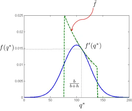
We briefly discuss the intuition behind the dependence of the bound (9) on the weighted mean
spread. The AMS ∆(q∗) can be thought of as a measure of dispersion around q∗. Note that the
slope C′(q) =−b + (b + h)F (q) is zero at q∗. How fast the slope changes depends on how fast the
distribution changes around the neighborhood of q∗. In other words, a distribution whose mass is
concentrated around q∗(i.e., has a small AMS) has a cost function C with a steeper slope around q∗.
This is illustrated in Figure 2. The left plot shows the pdf of a Normal and a uniform distribution. The right plot shows the relative regret (as a function of q) when b = h = 5 and the optimal order
0 50 100 150 200 0 0.002 0.004 0.006 0.008 0.01 0.012 0.014 0.016 q f Uniform Normal
(a) Probability density function
90 95 100 105 110 0 0.02 0.04 0.06 0.08 0.1 0.12 q C(q)/C(q*) − 1 Uniform, ∆(q*)=31.33 Normal, ∆(q*)=39.89 (b) Relative error Figure 2 Newsvendor problem with (b = 5, h = 5) for a uniform and normal distribution.
quantity is 100 units for both distributions. The uniform distribution, which has a smaller AMS, has a steeper relative regret function. The decision of ordering 110 units has a larger relative regret under the uniform distribution. Hence, distributions with a small AMS value incur a larger relative regret for deviating from the optimal order quantity. On the other hand, the size of the confidence
interval for the quantile estimator of q∗ is inversely proportional to f (q∗) (Asmussen and Glynn
2007). Thus, if f (q∗) is small, a larger sample size is needed for the quantity ˆQ
N to be close (in
absolute terms) to q∗. Therefore, if a distribution has a small weighted mean spread ∆(q∗)f (q∗),
then the SAA solution ˆQN is likelier to incur a large relative regret.
The new WMS-based bound predicts that the probability the SAA single-period relative regret exceeds ϵ decays exponentially in O(ϵ). This rate of decay is significantly faster than the best
known bound by Levi et al. (2007) which predicts this probability to decay exponentially in O(ϵ2).
However, computing the WMS-based bound requires information on the weighted mean spread of the underlying demand distribution. In the next section, we shall develop a new optimization framework to obtain a lower bound on the WMS for a family of distributions. Combined with Theorem 3, this results in a uniform probability bound for the SAA heuristic that is independent of distribution parameters when the demand distribution belongs to this family.
4. Optimization-Driven Bound on WMS
Suppose that the demand distribution f is such that it belongs toF, where F is a specified family
of distributions. Suppose v∗ is a lower bound on the weighted mean spread ∆(q∗)f (q∗) of any
distribution inF. Suppose we choose to bias ˜Qα
N, as defined in (8), by the factor α =
√
With minor changes to the proof of Theorem 3, we can show that C( ˜Qα
N)≤ (1 + ϵ)C(q∗) with
probability at least 1− 2U∗(ϵ), where
U∗(ϵ)∼ exp , −1 4N ϵv ∗ -, as ϵ→ 0.
Note that both the bias factor and this new bound does not depend on specific parameters of the
distribution beyond v∗. That is, unlike the bound in Theorem 3 which depends on the weighted
mean spread, this bound is independent of any distribution parameters.
We introduce an optimization framework to find a lower bound v∗ for a family of distributions
F. This is accomplished by the following optimization problem: inf f,q∗ ∆(q ∗)f (q∗) s.t. f∈F, 3 q∗ −∞ f (s)ds = b b + h. (10)
Note that q∗ is a decision variable, but because of the second constraint, it is forced to take the
value of the b
b+h quantile. Hence, (10) finds a distribution in F with the smallest WMS at the
b b+h
quantile. Solving (10) or finding a lower bound v∗on its optimal value provides a probability bound
for the relative regret of ˜Qα
N over all demand distributions that belong to F.
In what follows, we will restrict our attention to the family of log-concave distributionsL, which
includes many of the distributions commonly used in inventory theory (Zipkin 2000). We shall
show that if F = L, then (10) can be solved in closed form. Moreover, the resulting probability
bound on the relative regret incurred by the SAA solution is significantly tighter than the LRS bound (5).
Definition 3 (Log-Concave Distribution). A distribution f with support X is log-concave if
log f is concave inX .
It is known that the Normal distribution, the uniform distribution, the logistic distribution, the extreme-value distribution, the chi-square distribution, the chi distribution, the exponential distribution, and the Laplace distribution are all log-concave for any respective parameter values. Some families have log-concave density functions for some parameter regimes and not for others. Such families include the gamma distribution, the Weibull distribution, the beta distribution and
the power function distribution. Note that L is not characterized through any parameterization
(i.e, it does not depend on distributional parameters such as moments that need to be estimated), but rather describes properties satisfied by many common distributions.
Log-concave distributions are necessarily unimodal (Chandra and Roy 2001). Any distribution in this class must also have monotonic failure rate and reversed hazard rate (see Definition 4 below).
Definition 4 (Failure Rate and Reversed Hazard Rate). The failure rate is defined as
f
1−F. The reversed hazard rate is defined as
f F.
Log-concave distributions have both an increasing failure rate (IFR) and decreasing reversed hazard rate (DRHR). Intuitively, this implies that the distribution falls off quickly from its mode.
When we introduced our new analysis in Section 3, we made the technical assumption that f is continuous everywhere. In fact, if f is log-concave, then it can have at most one jump discontinuity, and the jump can only occur at the left end-point of its support (Sengupta and Nanda 1997). Therefore, assuming that the demand distribution is log-concave automatically implies that this continuity assumption is also satisfied.
4.1. Probability Bound for Log-Concave Distributions
To solve (10) for log-concave distributions, we first solve a constrained version of (10). Specifically,
for some γ0> 0 and γ1, fix the value of q∗ and add the constraints f (q∗) = γ0 and γ1∈ ∂ log f(q∗),
where ∂ log f (q∗) is the set of all subgradients of log f at q∗. The following optimization problem
is obtained: min f b + h h 3 ∞ q∗ sf (s)ds−b + h b 3 q∗ −∞ sf (s)(ds) s.t. f∈L, 3 q∗ −∞ f (s)ds = b b + h, f (q∗) = γ 0, γ1∈ ∂ log f(q∗). (11)
Note that since the density value f (q∗) is fixed, the objective of the constrained problem reduces
to minimizing the absolute mean spread ∆(q∗). The following lemma provides necessary conditions
on values of γ0 and γ1 for the feasible set of (11) to be nonempty. The proof is provided in the
electronic companion.
Lemma 1. Let f be a log-concave pdf. Suppose q∗ is the b
b+h quantile with f (q∗) = γ0 and γ1∈
∂ log f (q∗) for some γ
0> 0 and γ1. Then−b+hh ≤γγ10 ≤b+hb .
Solving the constrained problem (11) for log-concave distributions proves to be much simpler than solving (10). We shall first show that the optimal value of (11) is attained by an exponential-type distribution. As a consequence, we are able to obtain a uniform lower bound for the WMS of
any log-concave distribution. Particularly, we show that ∆(q∗)f (q∗)≥min(b,h)
b+h .
To solve (11), we note that for a log-concave distribution f , specifying a value for a subgradient of log f bounds how fast the pdf f can grow or decay. This is formalized in the next lemma. The proof is provided in the electronic companion.
Lemma 2. Let f be a log-concave pdf. Suppose that for some t in its support, f (t) = γ0 and γ1∈
∂ log f (t). Then for any x, f (x)≤ γ0eγ1(x−t).
In fact, the upper bound in Lemma 2 is sufficient to obtain the optimal solution to (11). The next
lemma characterizes useful conditions that imply the AMS of one random variable D2 is lower than
another random variable D1. The proof is given in the electronic companion.
Lemma 3 (Domination Lemma). Let f1 and f2 be two pdfs, with respective cdfs F1 and F2.
Suppose that f1(x)≤ f2(x) for all x with f2(x) > 0, and that for some t, F1(t) = F2(t). Then
∆1(t)≥ ∆2(t), where ∆1 and ∆2 are the respective AMS of f1 and f2.
Finally, the following proposition constructs the optimal solution to optimization problem (11).
Proposition 1. Let Lq∗,γ0,γ1 be the set of all log-concave distributions with
b
b+h quantile q∗, and
f (q∗) = γ
0 and γ1∈ ∂ log f(q∗). The distribution with the smallest AMS ∆(q∗) inLq∗,γ0,γ1 is:
˜ f (x) = γ0eγ1(x−q ∗) , ∀x ∈ [x, x], (12) where x = q∗+ 1 γ1log / 1−γ1 γ0 b b+h 0 and x = q∗+ 1 γ1 log / 1 +γ1 γ0 h b+h 0 .
Proof. Note that ˜f is log-concave and therefore belongs in the set Lq∗,γ0,γ1. The range of ˜f
is well-defined since by Lemma 1, we have that γ1
γ0 ∈ ! −b+h h , b+h b "
. From Lemma 2, we know that ˜
f (x)≥ f(x) for all x ∈ [x, x] for each f ∈Lq∗,γ0,γ1. Thus, by the Domination Lemma 3, ˜f has a
smaller AMS than any f∈Lq∗,γ0,γ1, and is therefore the optimal solution to problem (11). Q.E.D.
A graphical illustration of the distribution ˜f in (12) is given in the electronic companion to this
paper (Figure EC.1). Finally, using the optimal value for problem (11), we are able to derive a uniform lower bound on the WMS of any log-concave distribution. To do this, we will need the following Lemma 4. The proof is provided in the electronic companion.
Lemma 4. Let β∈ (0, 1) and η ∈/− 1
1−β, 1 β
0
. Then, the following relationships are true: , 1 1− β+ η -log (1 + η(1− β)) + , 1 β− η -log (1− ηβ) − min{β, 1 − β}η2 ≥ 0, β 1− βlog , 1 β -− β ≥ 0, 1− β β log , 1 1− β -− (1 -− β) ≥ 0.
Proposition 2. Suppose D has a log-concave pdf f , with b
b+h quantile q∗ and AMS ∆(q∗). Then
∆(q∗)f (q∗)≥min(b,h) b+h .
Proof. Suppose that f belongs to the set Lq∗,γ0,γ1, i.e., it has a b+hb quantile q∗ with f (q∗) = γ0
and γ1∈ ∂ log f(q∗). Denote the optimal value of problem (11) by zq∗∗,γ0,γ1. From Proposition 1, the
distribution ˜f defined in (12) is the optimal solution of problem (11), which achieves the minimum
AMS z∗
q∗,γ0,γ1. We consider three cases. If γ1 γ0 ∈ & −b+h h , b+h b ' , then z∗ q∗,γ0,γ1= γ0 γ2 1 4, b + h h + γ1 γ0 -log , 1 +γ1 γ0 h b + h -+ , b + h b − γ1 γ0 -log , 1−γ1 γ0 b b + h -5 . If γ1 γ0 = b+h b , then z∗q∗,γ0,γ1=γ10 b hlog &b+h b ' . If γ1 γ0 =− b+h h , then z∗q∗,γ0,γ1=γ10 h blog &b+h h ' . By applying Lemma 4 with η =γ1 γ0 and β = b
b+h, we find that in all three cases zq∗∗,γ0,γ1≥γ10
min(b,h)
b+h . Since f is a
feasible solution of problem (11), we have that ∆(q∗)≥ z∗
q∗,γ0,γ1 ≥ 1 γ0 min(b,h) b+h = 1 f (q∗) min(b,h) b+h . Q.E.D.
Recall our original objective is to find the smallest WMS among distributions in the set L. To
do this we partitioned the set into subsets Lq∗,γ0,γ1. The derivation of Proposition 2 implies that
even solving the problem (11) restricted to a subset Lq∗,γ0,γ1, regardless of the value of γ1, the
minimum absolute mean spread is always bounded below by a term that only depends on b, h
and γ0. Hence, we are able to prove that min(b,h)b+h is a uniform lower bound on the weighted mean
spread for any log-concave distribution. Finally, this implies a probability bound for log-concave distributions. The proof is in the electronic companion.
Theorem 4 (Log-concave bound). Consider the newsvendor problem with underage cost b > 0
and overage cost h > 0. Suppose that D is log-concave and satisfies Assumption 1. Let ˜Qα
N be defined
as in (8), with α =62ϵbhminb+h{b,h}+ O(ϵ). Then for a given ϵ > 0, ˜Qα
N is ϵ-optimal with probability
of at least 1− 2U∗(ϵ), where U∗(ϵ)∼ exp , −1 4N ϵ min{b, h} b + h -, as ϵ→ 0. (13)
We point out a few nonparametric tests proposed in the literature that check whether a sam-ple has been drawn from a log-concave distribution. An (1995) proposes to test two necessary conditions for log-concavity. Another test proposed by Sengupta and Paul (2005) involves finding the Least Concave Majorant (LCM) to the log of empirical probability distribution function. The distribution is log-concave with high probability if the “distance” between the LCM and the log of the distribution function does not exceed a threshold.
Theorems 3 and 4 require that f (q) is decreasing for all q≥ q∗ (Assumption 1). We can in fact
use the log-concave statistical tests to check if this true. The advantage of the test by Sengupta and Paul (2005) is that it estimates the mode of the log-concave distribution (every log-concave distribution is unimodal). If the cumulative density at the estimated mode is significantly smaller
than b
Finally, we would like to stress that the insights from our results are not limited to log-concave distributions. In fact, if we can find a lower bound on the weighted mean spread of any distribution family, then we can bound the relative error of the SAA procedure applied to a distribution in that family.
5. Implications of the WMS-Based Bound
In Section 3, we derived a bound on the probability that the SAA quantity is ϵ-optimal. This derivation uses a novel analysis that is based on a tight approximation of the set of ϵ-optimal quantities. In this section, we study the implications of this new bound. First, we test whether the new WMS-based bound can match the empirical accuracy of SAA better than the previous bound by (Levi et al. 2007). Second, we study whether the WMS-based bound predicts the empirical relationship between the relative regret and sample size or relative regret and weighted mean spread. Third, we analyze the implications of the WMS-based bound on the cumulative regret of SAA over several time periods in a repeated newsvendor setting.
5.1. Empirical Accuracy of the SAA Heuristic
We conduct computational experiments to determine the empirical accuracy of the SAA heuristic. In the experiments, 1000 random independent samples (with a sample size of N = 100) are drawn
from a demand distribution. The respective SAA solutions {ˆq1
100, . . . , ˆq1001000} are computed, where
ˆ qi
100 is the SAA solution corresponding to random sample i. We note that although the sample
is drawn from specific distributions, the SAA solution is computed purely based on the resulting
empirical distribution. The respective relative regret of the SAA solutions are{ϵ1, . . . , ϵ1000} where
ϵi!C(ˆqi100)−C(q∗)
C(q∗) . We refer to the fraction of sets that incur a relative regret less than the target ϵ
to be the empirical confidence.
Using Theorem 2, we can infer the sample size required by the LRS bound to match the empirical confidence level. Table 1 summarizes the results of the outlined experiment for a newsvendor critical
quantile of 0.9. Rows labeled NLRS correspond to the LRS sample size. One can see from the
table that if, for example, the SAA counterpart is solved with a sample drawn from a uniform distribution, the relative errors are less than 0.02 in 81.8% of the sets. However, to match this same error and confidence level, the LRS bound requires a sample size of 1,088,200. The results of this experiment demonstrate that the LRS bound is not tight since the same accuracy and confidence probability can be achieved with a smaller sample size of 100. This large mismatch between the empirical SAA accuracy and the theoretical guarantee by the LRS bound prevails throughout various target errors ϵ and distributions.
Table 1 Theoretical bounds and actual empirical performance of SAA with N = 100. Note: “Emp conf” refers to the proportion of random samples where the SAA solution incurs relative regret less than ϵ.
Distribution ϵ = 0.02 ϵ = 0.04 ϵ = 0.06 ϵ = 0.08 ϵ = 0.10
Uniform Emp conf 81.8% 93.7% 96.6% 99.0% 98.9%
(A = 0, B = 100) NLRS 1,088,200 395,900 209,200 154,300 97,800
Nf 956 692 544 428 416
Normal Emp conf 75.8% 89.7% 94.7% 97.3% 99.4%
(µ = 100, σ = 50) NLRS 958,830 339,630 186,370 125,390 109,210
Nf 3,812 2,676 2,184 1,940 2,096
Exponential Emp conf 69.6% 84.4% 91.5% 94.0% 98.2%
(µ = 100) NLRS 855,280 292,090 162,120 102,130 88,560
Nf 1,472 996 824 684 736
Lognormal Emp conf 75.1% 90.5% 96.5% 98.2% 98.7%
(µ = 1, σ = 1.805) NLRS 945,890 348,880 207,670 137,190 94,680
Nf 1,272 932 824 720 616
Pareto Emp conf 79.1% 92.6% 98.0% 98.1% 99.5%
(xm= 1, α = 1.5) NLRS 1,025,400 377,500 236,400 135,600 112,600
Nf 1,152 840 780 592 612
In the same experiment, we use Theorem 3 to infer the sample size required by the new WMS-based bound to match the SAA accuracy. The results are reported in Table 1 under the rows labeled
Nf. We observe that the sample sizes predicted using the WMS-based analysis are empirically
significantly smaller than that of the LRS analysis. NLRS typically has an order of magnitude
between 100,000 to 1 million, whereas Nf is typically between 100 to 1,000. Hence, the new
WMS-based analysis results in a theoretical guarantee that is a better match to the empirical accuracy observed for the SAA heuristic.
5.2. Empirical Regret–Sample Size and Regret–WMS Relationship
In the next set of experiments, we use regression analysis to estimate the empirical relationship observed between: (i) relative regret and sample size, and (ii) relative regret and weighted mean square.
We empirically estimate the regret–sample size relationship by estimating parameters C, k in the
equation ϵ = CNk in a regression model from error data resulting from applying SAA to different
sample sizes. We fix a 90% confidence level and cost parameters h = 1 and b. The sample size N is
varied from {100, 200, . . . , 1000}. For each N, a total of 1000 random samples of size N are drawn
from a distribution. The SAA solutions{ˆq1
N, . . . , ˆq1000N } are calculated, and the resulting errors are
labeled {ϵ1
N, . . . , ϵ1000N } where ϵkN =
C(ˆqkN)−C(q∗)
C(q∗) . The 90% quantile of the errors is denoted by ϵN.
We perform the regression using the data {(100, ϵ100), (200, ϵ200), . . . , (1000, ϵ1000)}. Table 2 shows
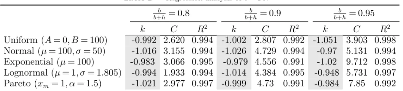
the estimated parameters as well as the R2 value. From Table 2, all estimates for k are close to -1,
Table 2 Regression analysis of ϵ = CNk b b+h= 0.8 b b+h = 0.9 b b+h = 0.95 k C R2 k C R2 k C R2 Uniform (A = 0, B = 100) -0.992 2.620 0.994 -1.002 2.807 0.992 -1.051 3.903 0.998 Normal (µ = 100, σ = 50) -1.016 3.155 0.994 -1.026 4.729 0.994 -0.97 5.131 0.994 Exponential (µ = 100) -0.983 3.066 0.995 -0.979 4.556 0.991 -1.02 9.712 0.998 Lognormal (µ = 1, σ = 1.805) -0.994 1.933 0.994 -1.014 4.384 0.995 -0.948 5.731 0.997 Pareto (xm= 1, α = 1.5) -1.021 2.977 0.997 -0.999 4.73 0.991 -0.984 7.85 0.992
Table 3 Regression analysis of ϵ = C{∆(q∗)f (q∗)}k
N k C R2
100 -0.843 0.0166 0.928
300 -0.939 0.0048 0.990
500 -0.947 0.0029 0.993
the WMS-based bound reflects the empirical regret–sample size accuracy size it predicts, ceteris paribus, that the regret is inversely proportional to the sample size.
Similar to the previous experiments, we estimate the empirical relationship between regret and
the weighted mean spread by estimating the parameters C, k in ϵ = C{∆(q∗)f (q∗)}k using a
regres-sion model on error data from SAA applied to different distributions with varying WMS values. We fix a 90% confidence level and a sample size N . We consider a pool of ten distributions, i.e., the five distributions in Table 2 each under two values of the newsvendor quantile, 0.9 and 0.95
(note that the WMS value depends on the newsvendor quantile). Let ωi be the weighted mean
spread of distribution i. A total of 1000 independent samples of size N are drawn from distribution
i. We denote by ϵi the 90% quantile of the errors of the 1000 SAA solutions. We perform the
regression using the data{(ω1, ϵ1), (ω2, ϵ2), . . . , (ω10, ϵ10)}. The results of the regression are reported
in Table 3 for different values of N . Based on the results, the R2 value is close to 1, signifying
that empirically there is a strong inverse relationship between the weighted mean spread and the relative regret. Hence, the WMS-based bound matches the empirical relationship of regret and WMS since it predicts, ceteris paribus, that regret is inversely proportional to the distribution’s weighted mean spread.
5.3. Cumulative Regret of SAA in a Repeated Newsvendor Setting
In a repeated newsvendor setting, where policy adapts based on additional demand information, a metric to evaluate the performance of a data-driven policy is the cumulative regret it incurs over consecutive time periods. Based on the WMS-based probabilistic bound for the single-period relative regret of the SAA, we can derive a bound on the cumulative regret of the SAA over N periods which is O(ln N ).
Note that the single-period regret of the SAA solution is a nonnegative random variable. Hence, we can compute a bound on the expected single-period regret by integrating the WMS-based probabilistic bound over all thresholds ϵ > 0. That is, suppose that an additional demand data is revealed in each period, then the expected regret of the SAA heuristic at time period t is
E/C/Qˆt 0 − C(q∗)0= C(q∗) ∞
3
0 Pr ⎛ ⎝C / ˆ Qt 0 − C(q∗) C(q∗) > ϵ ⎞ ⎠ dϵ ≤∆(q8C(q∗)f (q∗)∗)t= 8bh (b + h)f (q∗)t, (14) where the inequality results from applying the WMS-based bound in Theorem 3. Hence, the cumu-lative regret over N periods is:E ; N % t=1 / C/Qˆt 0 − C(q∗)0 < ≤ 8bh (b + h)f (q∗) N % t=1 1 t ≈ 8bh (b + h)f (q∗)ln N (15)
Hence, an implication of our analysis for the single-period regret implies that the SAA achieves an cumulative regret over N periods that is O(ln N ).
In a recent paper, Besbes and Muharremoglu (2013) show that if the demand distribution is continuous, then for any nonanticipating policy on uncensored demand, the worst-case cumulative regret cannot be smaller than O(ln N ). Hence, based on our upper bound (15), we conclude that the policy of ordering the SAA quantity in each time period results in a cumulative regret of O(ln N ), which matches the minimax cumulative regret derived by Besbes and Muharremoglu (2013).
This might seem surprising since under the censored demand setting, where the decision-maker has less information, Huh and Rusmevichientong (2009) introduce an adaptive data-driven policy (based on estimating the gradient from the censored demand) which incurs a cumulative regret that is also O(ln N ). However, as is shown in Besbes and Muharremoglu (2013), when demand is continuous, the minimax regret of both censored and uncensored demand cases is O(ln N ). As they state in their paper, “To achieve the best rate of growth of the minimax regret one does not need to actively explore, as a stochastic direction of cost improvement is available even when the demand samples are censored, and as a result, one may apply stochastic gradient type algorithms such as the [Huh and Rusmevichientong (2009)] policy.” We are able to show using our analysis that the commonly-used SAA approach similarly matches the cumulative regret O(ln N ) of the stochastic gradient policy.
In our analysis of the SAA solution, we had to assume that demand is continuous in order to approximate the ϵ-optimal set using Taylor series expansion around the critical quantile. Hence, the SAA’s cumulative regret of O(ln N ) only holds for continuous demand distributions. When the
demand distribution is discrete, Besbes and Muharremoglu (2013) are in fact able to show that the cumulative regret of the SAA policy does not depend on the number of time periods N . This is because when the support is discrete, one may identify the critical quantile exactly with very high probability, whereas for a continuous support, it is only possible to do so up to some error.
6. Empirical Comparison to Other Data-Driven Heuristics
In this section, we conduct computational experiments to compare the empirical accuracy of the
SAA solution vis-´a-vis other data-driven heuristics, and how accuracy of both methods compare.
The SAA heuristic estimates the unknown demand distribution with the empirical distribution formed by the sample. Another popular data-driven heuristic is a distribution-fitting approach. This heuristic infers the true distribution by fitting the sample to a distribution family the true distribution is assumed to belong. For instance, a common practice is to assume demand is normally distributed, and the sample is used to estimate its parameters. The argument for a distribution-fitting approach is that the tail of the distribution cannot be accurately approximated by the empirical cdf. Hence, when the critical quantile is close to 1, a distribution-fitting approach results in smaller ordering errors by hopefully better approximating the distribution tail. However, the distribution-fitting approach is sensitive to the specification of the distribution family. That is, if the true demand distribution is non-normal, then fitting the sample to a normal distribution might potentially result in a suboptimal order quantity. However, to reduce this risk it is possible to use distribution-fitting softwares, such as EasyFit, which finds the distribution that “best” fits the sample. EasyFit in particular has more than 50 distributions in its database, and chooses the distribution that has the smallest Kolmogorov-Smirnov statistic (based on the largest difference between the fitted distribution and the empirical cdf).
Consider the following experiment. A random sample is drawn from one of the following distri-butions: (i) an exponential distribution with mean µ = 100, (ii) a Normal distribution with mean
µ = 100 and standard deviation σ = 100, (iii) a Pareto distribution with scale parameter xm= 1
and shape parameter α = 1.5, (iv) a scaled beta distribution with range [0, 50] and shape param-eters α = 5, β = 1, and (v) a mixture of three Normal distributions where µ = (100, 500, 1000), the
standard deviation for each is σ = 100 and the weight vector is w = (5
9, 1 3,
1
9). The drawn sample is
used to generate two order heuristics. The first is the SAA order quantity, which is simply the b
b+h
quantile of the sample. The second is the Best Fit order quantity, which is the b
b+h quantile of the
distribution F chosen by the software EasyFit to be the “best” fit for the sample.
We conduct the experiment for sample size N ∈ {25, 50, 100, 200} and for cost parameters, where
we set h = 1, and vary b such that b
b+h∈ {0.1, 0.2, . . . , 0.9, 0.95, 0.99}. For a given b
b+h, 100 random
ˆ
qk is found through one of the heuristics (SAA or Best Fit). If q∗ is the true solution, then the
relative error of ˆqk is given by ϵk=C(ˆqk)−C(q∗)
C(q∗) . The average relative error of the heuristic is the
average of {ϵ1, . . . , ϵ100}. Tables EC.2, EC.3, EC.4, EC.5 and EC.6 in the electronic companion
present the average errors for different critical quantiles b
b+h and sample sizes N when the samples
are drawn from an exponential, a Normal, a Pareto, a beta distribution, and a mixture of Normal distributions, respectively.
We first analyze the effect of the shape of the distribution on the inaccuracy of the SAA method and the Best Fit method. Table EC.6 shows the average errors of the methods when the samples are drawn from a nonstandard distribution: a mixture of three Normal distributions. Note that when the sample size is at least 50, the average errors of the SAA heuristic is small (less than 5%, and in most cases less than 1%). The largest average error of the SAA heuristic is about 10%. However, the Best Fit method (which fits the data to standard distributions with at most two modes) show instances when the errors are 25% or even 30%. This suggests that, overall, the SAA method can handle nonstandard distributions better than the Best Fit heuristic, especially if the available demand data is limited.
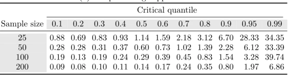
We next observe the effect of the sample size on the accuracy of the two heuristics. The cases when the inaccuracy of the solution from the SAA method is most apparent is when the newsvendor
quantile is large, e.g. b
b+h = 0.99, while the sample size is small. In fact, we observe that when
estimating a quantile that corresponds to a rare event (characterized by a small density), the sample size must be sufficiently large (usually N = 100 or more) for the average errors to be small. When N = 200, the average errors are uniformly small for all distributions.
7. Conclusions
The sample average approximation (SAA) method is a simple and powerful tool for solving stochas-tic optimization problems without knowing the distribution. It relies only on observing a sample drawn from the true distribution. Due to its simplicity, it is often used in practice when solving distribution-free stochastic optimization problems. This work derived a bound on the probability that the SAA solution applied to the newsvendor problem has a relative regret exceeding a spec-ified threshold. The bound was derived through a novel analysis which approximates the set of ϵ-optimal solutions to the newsvendor model through gradient information. Unlike the distribution-free bound of Levi et al. (2007), the new bound derived in this work depends on the demand distribution’s weighted mean spread (WMS). Hence, it is significantly tighter and can match the empirical accuracy of the SAA observed in many computational experiments. We also derived a distribution parameter-free bound for the family of log-concave distributions using an optimiza-tion framework which minimizes the WMS over the family. This optimizaoptimiza-tion framework can be
also applied to other interesting distribution families, which seems to be a promising future direc-tion. Other potential future directions are to extend the analysis to an objective function that is piecewise linear, or to introduce a weighted mean spread for a multivariate demand distribution.
Acknowledgments
The authors thank the associate editor and two anonymous referees for their insightful comments which have significantly improved this paper. The research of the first author was partially supported by NSF grants DMS-0732175 and CMMI-0846554 (CAREER Award), AFOSR awards FA9550-08-1-0369 and FA9550-11-1-0150, a Singapore-MIT Alliance (SMA) grant, and the Buschbaum Research Fund of MIT. The research of the second author was partially supported by NSF grants CMMI-0824674 and CMMI-0758061 and a Singapore-MIT Alliance (SMA) grant. The research of all three authors was partially supported by BP.
References
A. Akcay, B. Biller, and S. Tayur. Improved inventory targets in the presence of limited historical demand data. Tepper School of Business Working Paper, Carnegie Mellon University, Pittsburgh, PA, 2009. M.Y. An. Log-concave probability distributions: theory and statistical testing. Technical Report, Economics
Department, Duke University, Durham, NC, 1995.
S. Asmussen and P. Glynn. Stochastic simulation: algorithms and analysis, chapter 4, pages 77–80. Springer, New York, 2007.
M. Ball and M. Queyranne. Toward robust revenue management: competitive analysis of online booking. Operations Research, 57:950–963, 2009.
S. N. Bernstein. Theory of Probability. Moscow, 1927.
O. Besbes and A. Muharremoglu. On implications of demand censoring in the newsvendor problem. Man-agement Science, 59(6):1407–1424, 2013.
J. H. Bookbinder and A. E. Lordahl. Estimation of inventory reorder level using the bootstrap statistical procedure. IEE Transactions, 21:302–312, 1989.
N. K. Chandra and D. Roy. Some results on reversed hazard rate. Probability in the Engineering and Informational Sciences, 15:95–102, 2001.
S. Eren and C. Maglaras. Revenue management heuristics under limited market information: A maximum entropy approach. Presented at The 6th Annual INFORMS Revenue Management Conference, Jun 5-6, Columbia University, 2006.
A. D. Flaxman, A. T. Kalai, and H. B. McMahan. Online convex optimization in the bandit setting: Gradient descent without a gradient. In Proceedings of the sixteenth annual ACM-SIAM symposium on Discrete algorithms, SODA ’05, pages 385–394, 2005.
G. Gallego and I. Moon. The distribution free newsboy problem: Review and extensions. Journal of the Operational Research Society, 44(8):825–834, 1993.
P. Glasserman and Y. C. Ho. Gradient Estimation via perturbation analysis. Kluwer Academic Publishers, 1991.
G. A. Godfrey and W. B. Powell. An adaptive, distribution-free algorithm for the newsvendor problem with censored demands, with applications to inventory and distribution. Management Science, 47: 1101–1112, 2001.
W. Hoeffding. Probability inequalities for sums of bounded random variables. Journal of the American Statistical Association, 58:13–30, 1963.
T. Homem-De-Mello. Monte carlo methods for discrete stochastic optimization. In S. Uryasev and P. M. Parados, editors, Stochastic Optimization: Algorithms and Applications, pages 95–117. Kluwer Aca-demic Publishers, Norwell, MA, 2000.
W. T. Huh and P. Rusmevichientong. A nonparametric asymptotic analysis of inventory planning with censored data. Mathematics of Operations Research, 34:103–123, 2009.
W. T. Huh, R. Levi, P. Rusmevichientong, and J. Orlin. Adaptive data-driven inventory control policies based on Kaplan-Meier estimator. Working paper, 2008.
A. J. Kleywegt, A. Shapiro, and T. Homem-De-Mello. The sample average approximation method for stochastic discrete optimization. SIAM Journal on Optimization, 12:479–502, 2001.
R. Levi, R. Roundy, and D. B. Shmoys. Provably near-optimal sampling-based policies for stochastic inven-tory control models. Mathematics of Operations Research, 32(4):821–839, 2007.
R. Levi, G. Perakis, and J. Uichanco. Regret optimization for stochastic inventory models with spread information. Working paper, 2011.
L. H. Liyanage and J. G. Shanthikumar. A practical inventory control policy using operational statistics. Operations Research Letters, 33:341–348, 2005.
G. Perakis and G. Roels. Regret in the newsvendor model with partial information. Operations Research, 56:188–203, 2008.
R. T. Rockafellar. Convex Analysis. Princeton University Press, Princeton, NJ, 1972.
H. Scarf. Bayes solution to the statistical inventory problem. Annals of Mathematical Statistics, 30(2): 490–508, 1959.
H. E. Scarf. A min-max solution to an inventory problem. In K. J. Arrow and S. Karlin and H. E. Scarf, editor, Studies in Mathematical Theory of Inventory and Production, pages 201–209. Stanford Univerity Press, Stanford, CA, 1958.
D. Sengupta and A. Nanda. Log-concave and concave distributions in reliability. Naval Research Logistics, 46:419–433, 1997.
D. Sengupta and D. Paul. Some tests for log-concavity of life distributions. Preprint available at http: //anson.ucdavis.edu/~debashis/techrep/logconca.pdf., 2005.
A. Shapiro. Stochastic programming approach to optimization under uncertainty. Mathematical Program-ming, 112:183–220, 2008.
C. Swamy and D. B. Shmoys. Sampling-based approximation algorithms for multi-stage stochastic optimiza-tion. In Proceedings of the 46th Annual IEEE Symposium on the Foundations of Computer Science, 2005.
Proofs, Tables and Figures
In this electronic companion to the paper, we provide proofs of the theorems and lemmas. This companion also contains several accompanying tables and figures to the paper.
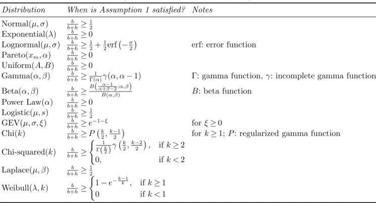
Table EC.1 Range of critical fractile values where Assumption 1 holds.
Distribution When is Assumption 1 satisfied? Notes
Normal(µ, σ) b b+h ≥ 1 2 Exponential(λ) b b+h ≥ 0 Lognormal(µ, σ) b b+h ≥ 1 2+ 1 2erf & −σ 2 '
erf: error function
Pareto(xm, α) b+hb ≥ 0 Uniform(A, B) b b+h ≥ 0 Gamma(α, β) b b+h ≥ 1
Γ(α)γ(α, α− 1) Γ: gamma function, γ: incomplete gamma function
Beta(α, β) b b+h ≥ B(α+βα−1 −2;α,β) B(α,β) B: beta function Power Law(α) b b+h ≥ 0 Logistic(µ, s) b b+h ≥ 1 2 GEV(µ, σ, ξ) b b+h ≥ e−1−ξ for ξ≥ 0 Chi(k) b b+h ≥ P &k 2, k−1 2 '
for k≥ 1; P : regularized gamma function
Chi-squared(k) b b+h ≥ = 1 Γ(k2)γ &k 2, k−2 2 ' , if k≥ 2 0, if k < 2 Laplace(µ, β) b b+h ≥ 1 2 Weibull(λ, k) b b+h ≥ = 1− e−k−1k , if k≥ 1 0 if k < 1
Table EC.2 Average errors (%) with samples from an exponential distribution.
(a) Sample average approximation Critical quantile Sample size 0.1 0.2 0.3 0.4 0.5 0.6 0.7 0.8 0.9 0.95 0.99 25 2.39 1.83 2.08 2.24 2.62 3.22 4.05 4.67 7.65 10.87 33.76 50 0.77 0.73 0.81 0.87 1.35 1.49 1.93 2.38 3.10 7.33 16.89 100 0.54 0.34 0.48 0.60 0.70 0.91 0.96 1.50 2.03 3.24 8.56 200 0.27 0.23 0.27 0.29 0.34 0.40 0.49 0.64 1.22 2.22 4.36 (b) Distribution fitting Critical quantile Sample size 0.1 0.2 0.3 0.4 0.5 0.6 0.7 0.8 0.9 0.95 0.99 25 1.88 1.54 1.54 1.69 2.03 2.60 3.37 4.26 5.81 9.64 40.06 50 0.65 0.64 0.69 0.80 0.99 1.23 1.53 1.90 2.72 4.88 22.93 100 0.36 0.34 0.39 0.46 0.57 0.73 0.96 1.33 1.91 2.62 9.03 200 0.21 0.20 0.21 0.24 0.28 0.34 0.43 0.59 0.94 1.64 7.25
Figure EC.1 Upper bound for a log-concave distribution with b
b+h quantile q∗.
Table EC.3 Average errors (%) with samples from a normal distribution.
(a) Sample average approximation Critical quantile Sample size 0.1 0.2 0.3 0.4 0.5 0.6 0.7 0.8 0.9 0.95 0.99 25 6.03 3.84 3.81 3.11 2.60 2.95 3.50 4.91 6.23 8.71 42.85 50 2.31 1.69 1.62 1.58 1.41 1.60 1.59 2.06 3.26 4.57 13.76 100 1.63 1.15 0.92 0.86 0.83 0.75 0.92 1.08 1.56 2.18 5.94 200 0.81 0.45 0.38 0.36 0.30 0.29 0.38 0.47 0.81 1.41 3.65 (b) Distribution fitting Critical quantile Sample size 0.1 0.2 0.3 0.4 0.5 0.6 0.7 0.8 0.9 0.95 0.99 25 4.65 3.53 3.07 2.73 2.62 2.77 3.16 3.74 5.48 12.83 75.12 50 1.91 1.43 1.27 1.20 1.24 1.38 1.60 1.87 2.53 4.41 18.77 100 1.13 0.90 0.78 0.71 0.68 0.69 0.76 0.89 1.17 1.75 6.59 200 0.47 0.36 0.28 0.25 0.25 0.27 0.33 0.42 0.63 1.03 3.92