Land Use in LCA (Subject Editor: Llorenç Milà i Canals)
Assessment of Land Use Impacts on the Natural Environment
Part 2: Generic Characterization Factors for Local Species Diversity in Central Europe
Thomas Koellner* and Roland W. Scholz
Swiss Federal Institute of Technology, Department of Environmental Sciences, Natural and Social Science Interface (ETH-NSSI), ETH-Zentrum CHN, 8092 Zurich, Switzerland
* Corresponding author ([email protected])
Part 1: An analytical framework for pure land occupation and land use change [Int J LCA 12 (1) 16–23 (2007)] Part 2: Generic characterization factors for local species diversity in Central Europe [Int J LCA 13 (1) 32–48 (2008)] Preamble. This series of two papers is based on a PhD thesis (Koellner 2003) and develops a method how to assess land use impacts on
biodiversity in the framework of LCA. Part 2 rests on a much richer database compared to the thesis in order to quantify generic characterization factors for local species' richness. Part 1 further expands the analytical framework of the thesis for pure land occupation and land use change.
indicating that the skewedness of the distribution is low. Stan-dard error is low and is similar for all intensity classes. Linear transformations of the relative species numbers are linearly
trans-formed into ecosystem damage potentials (EDPlinear
S ). The
inte-gration of threatened plant species diversity into a more
differenti-ated damage function EDPlinearStotal makes it possible to differentiate
between land use types that have similar total species numbers, but intensities of land use that are clearly different (e.g., artificial meadow and broad-leafed forest). Negative impact values indicate
that land use types hold more species per m2 than the reference
does. In terms of species diversity, these land use types are supe-rior (e.g. near-to-nature meadow, hedgerows, agricultural fallow).
Discussion. Land use has severe impacts on the environment. The
ecosystem damage potential EDPS is based on assessment of
im-pacts of land use on species diversity. We clearly base EDPS
fac-tors on α-diversity, which correlates with the local aspect of spe-cies diversity of land use types. Based on an extensive meta-analysis of biologists' field research, we were able to in-clude data on the diversity of plant species, threatened plant
spe-cies, moss and mollusks in the EDPS. The integration of other
animal species groups (e.g. insects, birds, mammals, amphibians) with their specific habitat preferences could change the charac-terization factors values specific for each land use type. Those mobile species groups support ecosystem functions, because they provide functional links between habitats in the landscape.
Conclusions. The use of generic characterization factors in Life
Cycle Impact Assessment of land use, which we have developed, can improve the basis for decision-making in industry and other organizations. It can best be applied for marginal land use deci-sions. However, if the goal and scope of an LCA requires it this generic assessment can be complemented with a site-dependent assessment.
Recommendations and Perspectives. We recommend utilizing the
developed characterization factors for land use in Central Europe and as a reference methodology for other regions. In order to as-sess the impacts of land use in other regions it would be necessary to sample empirical data on species diversity and to develop region specific characterization factors on a worldwide basis in LCA. This is because species diversity and the impact of land use on it can very much differ from region to region.
Keywords: Generic assessment; impacts; land use; LCA; species
diversity
DOI: http://dx.doi.org/10.1065/lca2006.12.292.2
Please cite this paper as: Koellner T, Scholz RW (2008):
Assessment of Land Use Impacts on the Natural Environ-ment. Part 2: Generic Characterization Factors for Local Spe-cies Diversity in Central Europe. Int J LCA 13 (1) 32–48
Abstract
Goal, Scope and Background. Land use is an economic activity
that generates large benefits for human society. One side effect, however, is that it has caused many environmental problems throughout history and still does today. Biodiversity, in particu-lar, has been negatively influenced by intensive agriculture, for-estry and the increase in urban areas and infrastructure. Inte-grated assessment such as Life Cycle Assessment (LCA), thus, incorporate impacts on biodiversity. The main objective of this paper is to develop generic characterization factors for land use types using empirical information on species diversity from Cen-tral Europe, which can be used in the assessment method devel-oped in the first part of this series of paper.
Methods. Based on an extensive meta-analysis, with information
about species diversity on 5581 sample plots, we calculated char-acterization factors for 53 land use types and six intensity classes. The typology is based on the CORINE Plus classification. We took information on the standardized α -diversity of plants, moss and mollusks into account. In addition, threatened plants were considered. Linear and nonlinear models were used for the
cal-culation of damage potentials (EDPS). In our approach, we use
the current mean species number in the region as a reference, because this determines whether specific land use types hold more or less species diversity per area. The damage potential calcu-lated here is endpoint oriented. The corresponding
characteriza-tion factors EDPS can be used in the Life Cycle Impact
Assess-ment as weighting factors for different types of land occupation and land use change as described in Part 1 of this paper series.
Results. The result from ranking the intensity classes based on
the mean plant species number is as expected. High intensive forestry and agriculture exhibit the lowest species richness (5.7–
5.8 plant species/m2), artificial surfaces, low intensity forestry
and non-use have medium species richness (9.4–11.1 plant
spe-cies/m2) and low-intensity agriculture has the highest species
Introduction
Land use is an economic activity that causes many environ-mental problems. Consequently, land use has been intro-duced in LCA as impact category (Heijungs et al. 1997, Udo de Haes et al. 1999). In particular biodiversity has been nega-tively influenced by intensive agriculture, forestry and the increase of urban areas and infrastructure. The measure-ment of land use impacts on biodiversity, however, is a com-plex task, because a widely accepted definition of biodiversity does not exist. In LCA, some indicators were proposed for
species diversity and ecological diversity. Indicators for
spe-cies diversity include number/percentage of vascular plant species (Koellner 2000, Koellner 2003, Vogtländer et al. 2004), number/percentage of threatened vascular plant spe-cies (e.g. Goedkoop and Spriensma 1999, Koellner 2003, Müller-Wenk 1998), species accumulation rate (Koellner 2000, Lindeijer 2000) or probability of species occurrence (Wiertz van Dijk and Latour 1992). The following indica-tors were proposed for ecological diversity: Structural di-versity of forest habitats (Giegrich and Sturm 1996) and area/ percentage of rare ecosystems (Müller-Wenk 1998, Schenck 2001, Vogtländer et al. 2004). The usefulness of those ap-proaches for decision-makers in industry and administra-tion very much depends on the availability of basic ecologi-cal information from environmental sciences. At the same time the information provided must be functional and mean-ingful to decision-makers (Werner and Scholz 2002). We propose to develop a set of generic characterization factors, which express the potential damage for ecosystems or more specific for species diversity, being an important aspect of ecosystems. The main goal of this paper is to perform a meta-analysis on land use and species diversity and to propose a method for the assessment of land use impacts on species diversity on the local scale, which is consistent with the framework of LCA. Accordingly, the method must be ge-neric and is generally not site-dependent. Udo de Haes (2006) proposes to implement such generic weighting schemes of species assemblages of different types of land use in the frame-work of LCA. To address site-dependent impacts of land use other approaches like environmental impact assessment (EIA) are more appropriate. In order to provide decision-makers with ecological information, we quantify the poten-tial impact of 53 land use types (ranging from continuous urban to near-to-nature forestry) based on reliable, published data. We expand upon an existing meta-analysis for local species diversity (Koellner 2003) and calculate character-ization factors on the basis of empirical data from 5,581 plots. In the meta-analysis we differentiate between all plant species and threatened plant species, as well as moss and mollusks. Specific problems posed by a meta-analysis of spe-cies richness and land use types are addressed.
1 Method for Developing Characterization Factors for Species Diversity
1.1 Endpoint definition and indicators of species diversity For the quantification of land use impacts on species diver-sity in LCA it is essential to clearly define assessment end-points for the calculation of characterization factors labeled
Ecosystem Damage Potential with respect to species
diver-sity or in short EDPS. For operational integration of biodi-versity into LCA we proposed species dibiodi-versity for endpoint definition (Koellner 2000, Koellner 2003). Genetic diversity is not operational, because there is a severe lack of informa-tion about the impact of land use activities on the genetic diversity of populations and species. Ecological diversity is included indirectly, because in the chain of cause and effect, the homogenization of habitats (i.e., reduction of ecological diversity) is an intermediate factor that directly contributes to the reduction of species diversity.
Endpoints for species diversity should be defined on differ-ent scales. It is essdiffer-ential to distinguish between α-, β- and γ-diversity (in sensu MacArthur 1965, Whittaker 1972, Whitt-aker et al. 2001), because underlying ecological processes interplay on multiple scales (Levin 2000). The mean species diversity for a single land use type can be referred to as α-diversity. It is defined on the local scale for homogenous land use types (e.g. mean species number of 1 m2
planta-tions versus 1 m2 near-to-nature forests). β-Diversity is
de-fined from local to regional scales. In this paper it stands for the species turnover between sample plots of one land use type (Whittaker 1972, Whittaker et al. 2001). Generally, the value for β-diversity measures the species diversity be-tween sample plots. It is high when sample plots differ with respect to their species community. It is low when the spe-cies composition of sample plots is very similar. It increases as the diversity of habitats and, hence, the environmental heterogeneity increases (Alard and Podevigne 2000, Balva-nera et al. 2002, Whittaker 1972). In Switzerland, for ex-ample,β-diversity is large for pioneer and weed species and small for fertilized meadow species; this clearly reflects the degree of homogeneity of respective habitats (Koellner et al. 2004). Finally, the species diversity of an entire region is defined as γ-diversity and is a function of β-diversities at intraregional scales (Balvanera et al. 2002, Whittaker 1972). 1.2 Development of characterization factors for species
diversity
Quantifying species diversity is challenging because of diffi-culties in measuring species abundance and distribution (Magurran 1996). In experimental settings (e.g. Hector et al. 1999) and in landscape ecology (e.g. Wohlgemuth 1998) species richness (i.e., the number of species per sample plot) was used as a proxy for diversity. To overcome the problem of abundance measurement a probabilistic method has been used for estimating species diversity (Hurlbert 1971, Palmer 1990, Simberloff 1978). Based on the presence or absence of data on the species in the sample plots, they calculated the expected number of species using a rarefaction function. The discontinuous rarefaction function integrates data on the species' commonness or rarity in a given region. How-ever, data requirements for rarefaction functions are less demanding than for indices like the Shannon-Wiener Index (Shannon 1948) and the Simpson Index (Simpson 1949), both of which require data on abundance.
For reliable characterization factors, the nonlinearity of the relationship between area and species number should be taken into account. Models used for fitting species-area
samples portray a monotonically increasing curve, which is steep at the beginning and gradually becomes flat (He and Legendre 1996). That is to say that, the first deviation of the functions is decreasing. Three models are commonly used for such curves: the power model (Arrhenius 1921), the ex-ponential model (Gleason 1922, Gleason 1925), and the logistic model (Archibald 1949). We used the widespread power (log-log) model according to Arrhenius (1921)
S = cAz (1)
where S is the species number; A the area of the plot; pa-rameter c (measure for species richness) and papa-rameter z (measure for species accumulation rate). The transformed power model
lnS = lnc + zlnA (2)
shown in equation [2] has two parameters. The parameter ln c (y-intercept) indicates the species richness of a sample standardized for A = 1. The parameter z (slope) denotes spe-cies accumulation rates and was proposed as a measure for β-diversity (Koellner et al. 2004, Ricotta et al. 2002). 1.3 Data sources and calculation of α-diversity
The goal is to derive generic characterization factors for all types of land use. It was not possible to gather data on all species groups. Therefore, we have chosen the vascular plant species as a proxy for the total species richness. One reason for this choice is the existence of reliable data for a wide variety of land use types. In addition, vascular plant species constitute terrestrial ecosystems and its diversity correlates highly with other species groups' diversity (Duelli and Obrist 1998). To check for correlations, the numbers of moss and mollusk species were assessed, based on the plots from the Biodiversity Monitoring Switzerland (BDM 2004). In order to develop characterization factors for plant spe-cies richness of individual land use types we performed a meta-analysis of published investigations, most of them from vegetation science. Plant species and composition of the veg-etation types were investigated according to the methods from Braun-Blanquet. The distribution of samples of land use types and their sources are given in Table 1.
In order to standardize the species number S we used one single species-area relationship for all land use types. We adjusted the species-area relationship according to equation [2], which yields a straight regression line on a ln-ln scale fit-ting all empirical data. Next we calculated the standardized species number Slm² by shifting the data points, in parallel with
the regression line, to the standard area size. This eliminates the aspect of S that is attributable to area size. The stan-dardized species number Slm²for 1 m2 is calculated as
Slm² = Splot – ∆S (3)
where Splot is the species number measured on a plot of size
Aplot in the field (which varies between different empirical
studies used here) and ∆S is that part of the species number which can be attributed to the area rather than the land use types. It is calculated as
∆S = S'plot – S'1m²= cAplotz – cA1m²z (4)
where S'plot is the average species number for the area Aplot and S'1m²is the average species number for the standard area
A1m². The average species number takes all land use types into consideration and is calculated using the regression line (see Fig. 2). The species number standardized for 1 m2was
calculated as:
S1m² = Splot – c(Aplotz – A1m²z) (5) For each species group we calculated mean species number standardized for 1 m2, standard error of mean (calculated
asσ / √n), median, minimum and maximum of species num-ber. In order to compare the different species groups, we performed a correlation analysis on the number of species per group (plants, threatened plants, moss, and mollusks) and determined which correlations are significant.
The number of threatened species found in BDM was also taken into account. The reason for this is that the indicator average species number would underestimate the ecological value of ecosystem types, which carry few but species of any threat status. In Switzerland for example 31.5% of the 3,144 vascular plant species are extinct, endangered or vulnerable (BUWAL 2002, IUCN 2001), 13.6% are near threatened, and 48.8% of the species are not threatened (i.e. they are of the least concern in IUCN terms). Obviously the occurrence of those species should be weighted more. The necessary data for that were only available for land use plots investi-gated in the BDM (2004).
1.4 Data source and calculation of β-diversity
In order to calculate β-diversity we used the rarefaction func-tion (Koellner et al. 2004). This method allows species-area relationships to be constructed out of species lists per sample plot. The resulting curve is discontinuous since the calcula-tion is based on the hyper-geometrical distribucalcula-tion. The method gives the expected number of species if n out of N sample plots are randomly chosen. For comparison of the slope of the curves for different land use types the continu-ous power function was fitted to the rarefaction function. In order to calculate the rarefaction curves, a consistent set of data is needed. For each sample plot, both the species number and the complete species list must be known. In addition, a large number of sample plots are needed to as-sess the slopes reliably. Data were taken from the Biodiversity Monitoring Switzerland (BDM 2004). For only six out of 33 land use types 39 or more sample plots for each land use type were available. Since the species turnover was expected to be different for areas < 800 m above sea level and moun-tainous areas > 800 m data sets were split into these two groups. Some land use types (e.g. bare rock) occur in Swit-zerland only > 800 m.
1.5 Indicator for γ-diversity
γ-diversity refers to the total number of species in a given region. Land use types, which carry threatened species re-duce the probability that species become extinct and thus total number of species decreases in this region. In this sense the indictor average threatened species number on the local scale refers also to the γ-diversity. However, in this paper this indicator could not be calculated due to limited avail-ability of data, which are consistent with those for α- and β-diversity.
1.6 Conversion of effects into damage/benefits
Based on the empirical information on species diversity for specific land use types we develop the characterization fac-tor ecosystem damage potential (EDPS). In literature we found absolute species numbers, however, these are less meaningful than relative species numbers where a compari-son with a reference is made. Species richness on a biogeo-graphical scale varies remarkably. If one divides Europe into 4 diversity zones, the number of vascular plant species per 10,000 km2 ranges from 200 to 500 in northern Scandinavia
CO RIN E P lus ID (A d a m 1 995) (A lb ra ch t 1997) (B D M 2004 ) (B ig le r et a l. 19 98) (B ru el h e id e 19 95) (C a ll a u c h 1981) (D ö ri n g -M e d e ra k e 1 991) (E wa ld 1 997) (F lü ck ig er 19 99) (G rü tt n e r 19 90) (K is te n e ic h 199 3) (L ip s et al . 1997 ) (M a n z 199 7) (M u rma n n -K ri ste n 1987 ) (R e id l 19 89) (S c h re ib e r 1995 ) (S c h u lte 1 985) S c hw a b , unp ubl is he d (S uk opp 1 9 9 0 ) (W it tw er e t a l. 1997) (W o h lg em u th 1992 ) (Z e rb e 199 9) (v o n O h e im b 200 3) To ta l 111 5 10 50 65 112 32 59 61 152 113 24 3 27 114 17 17 121 5 29 24 58 122 18 41 32 3 94 125 26 26 132 3 3 134 10 10 141 1 75 35 111 142 16 2 18 211 82 103 88 148 46 120 587 221 4 48 52 222 9 9 231 168 214 462 100 63 61 1068 244 2 2 245 11 11 311 10 57 501 122 101 223 97 263 1374 312 15 87 72 40 49 263 313 27 92 172 63 56 410 314 51 27 78 321 89 78 120 4 40 331 322 30 6 36 324 16 44 60 331 2 2 332 42 42 333 31 31 411 5 5 412 1 28 605 634 511 5 5 Total 52 16 788 471 568 88 501 244 27 825 122 215 46 204 274 46 219 120 6 61 223 202 263 5581
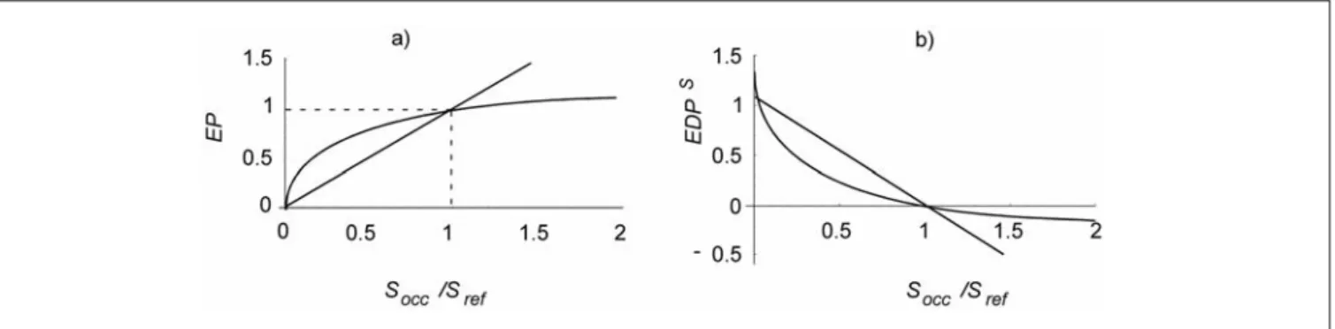
and from 2,000 to 3,000 in the southern parts of Mediterra-nean countries (Barthlott 1998, p. 36). Obviously, the im-pact of occupying a plot of land should be assessed relative to the region where the occupation takes place. Along a simi-lar vein of thought, Lindeijer proposed a map for reference states of plant diversity (2000). To calculate relative species numbers, we chose regional average species richness as a reference for assessing species richness of local plots. In order to further transform the empirical data on relative species diversity into characterization factors, we consid-ered two options for the effect-damage function: (1) a linear function and (2) a logarithmic one. Both functions are pur-ported to describe the functional relationship between spe-cies richness on a plot and ecosystem functions (Schläpfer and Schmid 1999) and are based on theories in ecosystem science (Schulze and Mooney 1994).
Option 1: Linear effect-damage function
The ecosystem damage potential for species diversity
EDP
linear Scan be calculated using a linear relationship as shown in Fig. 1b:
(6) where Socc is the species number of an occupied land use type and Sregion is the average standardized species number in the region. We took the Swiss Lowland as reference re-gion, which serves a proxy for Barthlott's diversity zone 5. As a consequence land use types with lower species number compared to the reference are treated as detrimental land use types and such with higher species number as beneficial land use types. This calculation is appropriate to account also for threatened species since each species is weighted equally. We calculated EDPlinearStotal as the unweighted sum of
EDPlinearSplants and EDP
linear
Sthreatened plants for each of 5582 local plots. Data
on threatened species were only available for a subset of 841 plots and threatened species were only found on 78 of these. The mean and standard error of mean was determined for each type of EDPlinearS .
Option 2: Nonlinear effect-damage function
The logarithmic function (Fig. 1) is supported by the redun-dant species hypothesis, that is, that the addition of one
spe-cies results in a decrease in the marginal growth of utility in terms of ecosystem processes. The logarithmic relationship was taken, because Schläpfer and Schmid (1999) created an expert questionnaire and compiled the results with the find-ing that this relationship is most likely. Ecosystem processes
EP are a function of relative species richness (see Fig. 1a)
(7) Based on the previous function the nonlinear function for
EDPS
nonlinear (see Fig. 1b) is calculated as
(8)
The parameters a and b in equation [8] were quantified based on the work of Schläpfer and Schmid (1999). Using as 0.27 for a and 1 for b as parameter estimates, the resulting curve (Fig. 1a) has the approximate shape Schläpfer and Schmid had suggested based on the survey of 39 experts. We used the resulting effect-damage curve to transform the relative species number is shown in Fig. 1b.
We calculated EDPnonlinearStotal as the unweighted sum of EDPnonlinearSplants , EDP
nonlinear
Smoss and EDP
nonlinear
Smollusks for a consistent set of
841 local plots from the Biodiversity Monitoring Switzer-land. Since a regional reference for moss and mollusks is missing, we took Sref of low intensity agriculture instead. 1.7 Classification of land use types
For the typology of land uses we applied the CORINE land cover classification (European Environmental Agency 2000). CORINE includes all the major land cover types in Europe and provides three different levels of classification. Some modifica-tions were necessary, because in their original form, the classi-fications did not distinguish between low-intensity land use and high-intensity land use. Especially for forestry and agri-culture, such distinctions are very important. For example the damage potential for forests, which are close-to-nature, and coniferous plantations is assumed to differ and should be sepa-rately assessed. The modified CORINE Plus classification (Koellner 2003) is given in Appendix 1 (see OnlineEdition, DOI: http://dx.doi.org/10.1065/lca2006.12.292.3, pp. 48-1-48-3).
Fig. 1: a) Linear and logarithmic relationships reflecting relative species richness (Socc is the species number on the occupied plot and Sref that of the
reference) and ecosystem processes EP. b) The corresponding effect-damage function for ecosystem damage potential EDPS
. The parameters of non-linear relationship [7] were based on Schläpfer et al. (1999)
2 Results for Characterization Factors of Land Use Types 2.1 Function of species-area relationship used for
standardization
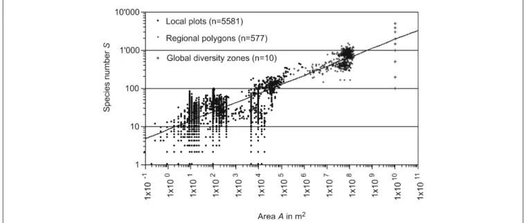
The size and species number of all local plots, regional poly-gons of Switzerland and global biodiversity zones are shown in Fig. 2. The standardized species number was calculated based on this graph. Based on the regression function [2], which has a correlation coefficient of R2 = 0.60, we can calculate S = 9.58A0.21 in m2. The regression was calculated
taking into account all local plots (homogenous land use types) and regional plots from Switzerland (species diversity for mix of land use types based on WSL/FNP without year).
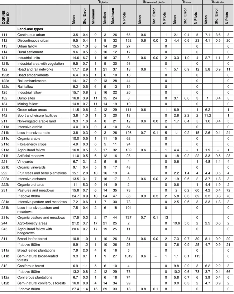
2.2 α-Diversity
The standardized α-diversity for vascular plants, threatened vascular plants, moss and mollusks differ between specific land use types, classes of intensity of land use (Table 2). In general, the standardized species number per m2 ranges from
3.8 species (sport facilities) to 27.4 species (semi-natural forests with 800 m above sea level). Three general classes of land use types can be distinguished:
• The species poor land use types (3.5–8 plant species/m2)
include sport facilities, continuous urban area, conven-tional arable land, intensive meadow, and coniferous plan-tations. The reason for the low species number, and thus, its low ecological value, is the high-intensity of land use. A mixture of intentional physical and/or chemical measures keeps the species number very low. Due to its low spe-cies number bare rock in the Swiss Alps above 800 m belongs also to this group, despite of the fact this natural habitat shows a high number of threatened species. • Some examples for land use types with medium species
richness (8–15 plant species/m2) are semi-natural
broad-leafed forest, organic arable land, and industrial areas with vegetation, green urban, and discontinuous urban
area. This group is quite heterogeneous in terms of natu-ralness and intensity of land use. For example, in artifi-cial meadows (11 plant species/m2), cultivation is very
intensive, whereas in broad-leaved forests (10.8 plant species/m2), human impact is less common and
inten-sive. Although the mean number of plant species is al-most equal, the forest habitat has more threatened plant species than artificial meadows do.
• Land use types with high species richness (15–28 plant species/m2) are industrial and agricultural fallow, organic
meadow, forest edges, agricultural fallow with hedge-rows, and natural grassland. This group is also hetero-geneous in terms of naturalness and land use intensity. One reason for the high species number is that land is generally not used intensively. Agricultural fallow with hedgerows and forest edges are species rich, because these land use types are heterogeneous in terms of abiotic con-ditions (e.g., light, moisture). Many land use types with threatened species can be found in this group.
The result from ranking the intensity classes based on the mean plant species number is as expected. High intensive forestry and agriculture exhibit the lowest species richness (5.7–5.8 plant species/m2), artificial surfaces, low intensity
forestry and non-use have medium species richness (9.4– 11.1 plant species/m2) and low-intensity agriculture has the
highest species richness (16.6 plant species/m2). The mean
and median are very close, indicating that the skewedness of the distribution is low. Standard error is low and is simi-lar for all intensity classes.
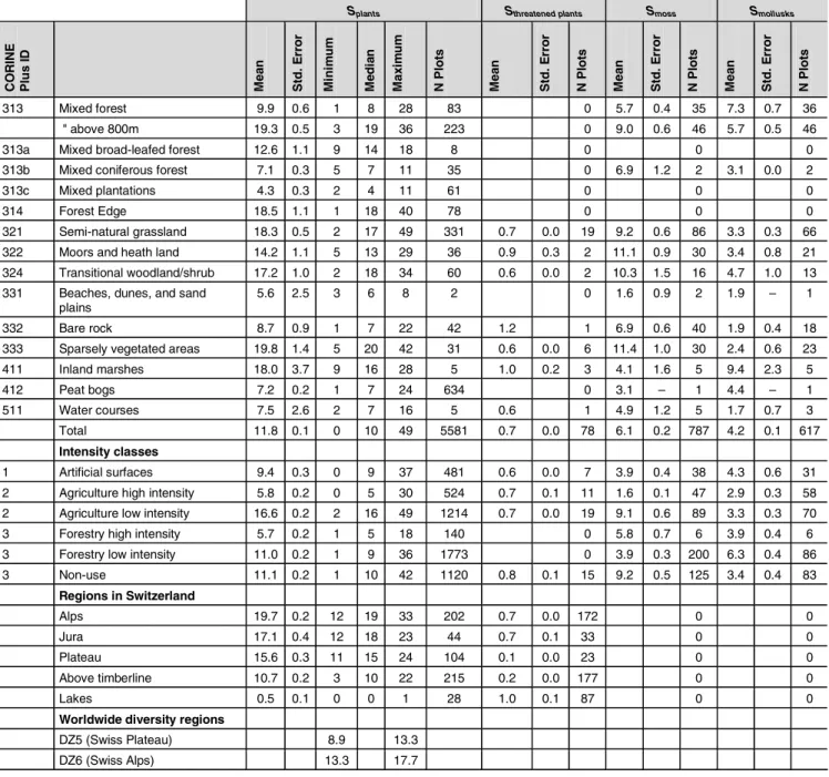
The data for moss and mollusk species is less certain than that for plant species. This is mainly attributable to there being a fewer number of sample plots per land use type, which leads to high standard errors. Those data, however, can be used to make distinctions between land use types, which are similar in plant species number, but very different in other species groups. For example, although the numbers
Fig. 2: Regression function (S = 9.58*A0.21, R2= 0.60) for the area in m2 and species number, taking local plots, regional polygons, and global diversity
Table 2: Standardized species numbers S (vascular plants, moss, mollusks) for specific land use types, intensity classes, and Swiss regions. The area
chosen for standardization was 1 m2. Calculated for Switzerland on the basis of the BDM data set, there are 1061 vascular species, 519 moss species, and 133 mollusk species
Splants Sthreatened plants Smoss Smollusks
CO R INE Pl u s I D Me a n Std . E rr o r Mi ni m u m Me d ia n Ma x im u m N P lot s Me a n Std . E rr o r N P lot s Me a n Std . E rr o r N P lot s Me a n Std . E rr o r N P lot s Land-use types 111 Continuous urban 3.5 0.4 0 3 26 65 0.6 – 1 2.1 0.4 5 7.1 3.6 3 112 Discontinuous urban 9.5 0.4 1 9 32 152 0.6 0.0 3 4.4 0.6 23 4.1 0.5 20 113 Urban fallow 15.5 1.0 8 14 29 27 0 0 0 114 Rural settlement 9.6 0.5 5 10 12 17 0 0 0 121 Industrial units 14.6 6.7 1 16 37 5 0.6 0.0 2 3.3 1.0 4 2.7 1.1 3 121b Industrial area with vegetation 9.5 0.7 1 9 20 53 0 0 0 122 Road and rail networks 17.7 2.9 1 21 37 18 0.6 1 5.1 0.9 12 5.8 0.9 11 122b Road embankments 6.4 0.6 1 6 10 13 0 0 0 122d Rail embankments 14.1 0.7 9 13 28 44 0 0 0 122e Rail fallow 9.2 0.5 6 9 13 19 0 0 0 125 Industrial fallow 15.7 0.8 8 16 22 26 0 0 0 132 Dump sites 16.8 3.9 11 15 24 3 0 3.1 0.6 3 1 0.4 3 134 Mining fallow 14.8 0.7 11 14 19 10 0 0 0 141 Green urban areas 11.5 0.6 2 12 29 111 0.6 – 1 6.9 – 1 6.2 – 1 142 Sport and leisure facilities 3.8 1.0 1 3 20 18 0 2.8 2.2 2 11.2 1 211 Non-irrigated arable land 9.3 1.6 4 8 21 12 0.6 0.0 2 1.7 0.4 5 1.6 0.4 5 211a Intensive arable 4.0 0.3 0 4 10 54 0 0 0 211b Less intensive arable 3.8 0.3 0 3 26 198 0.7 0.1 5 1.1 0.2 15 2.6 0.4 24 211c Organic arable 10.0 0.5 1 11 15 62 0 0 0 211d Fibre/energy crops 4.9 0.3 0 5 11 94 0 0 0 211e Agricultural fallow 16.8 0.5 5 17 32 139 0.6 – 1 4.4 – 1 1.9 – 1 211f Artificial meadow 11.0 0.5 6 12 16 28 0 1.8 0.2 22 3.3 0.5 23 221 Vineyards 6.7 3.1 2 5 16 4 0 0.6 1 4.8 1.4 4 221b Organic vineyards 9.1 0.4 5 9 17 48 0 0 0 222 Fruit trees and berry plantations 15.1 2.0 10 16 19 4 0 2.2 1.4 4 4.4 0.5 4 222a Intensive orchards 13.5 3.1 7 16 17 3 0.6 0.0 2 1.9 0.6 2 3.7 1.3 3 222b Organic orchards 14 5.3 9 14 19 2 0 0.6 1 4.4 1.9 2 231 Pastures and meadows 15.8 0.7 6 14 35 78 0 2 0.2 60 4.2 0.4 72
" above 800m 24.7 0.9 10 24 47 86 0.9 0.3 2 5.8 0.6 69 3.3 0.3 70 231a Intensive pasture and meadows 7.2 0.6 1 7 30 73 0 2.5 0.6 3 3.3 1.3 3 231b Less intensive pasture and
meadows
7.5 0.4 2 6 18 104 0 0 0 231c Organic pasture and meadows 17.5 0.3 2 17 44 727 0.7 0.1 13 0 0 244 Agro-forestry areas 21.2 3.7 17 21 25 2 0 10.6 5.0 2 2.5 0.6 2 245 Agricultural fallow with
hedgerows
20.6 0.7 17 19 25 11 0 0 0 311 Broad-leafed forest 10.8 1.0 1 10 26 31 0.6 0.0 2 7.3 0.7 30 8.1 0.9 29
" above 800m 9.9 1.2 1 10 26 26 0 7.6 0.9 25 4.7 0.9 21 311a Broad leafed plantations 7.9 2.0 4 6 16 5 0 0 0 311b Semi-natural broad-leafed
forests
9.3 0.1 1 9 27 1312 0.6 – 1 1.1 0.1 115 0 312 Coniferous forest 6.9 1.1 5 6 10 4 0 9.8 2.9 3 6.2 2.2 3
" above 800m 13.2 0.8 2 12 29 73 0 10.2 0.6 73 3.7 0.4 66 312a Coniferous plantations 6.7 0.3 1 6 18 74 0 5.8 0.7 6 3.9 0.4 6 312b Semi-natural coniferous forests 16.0 0.8 4 14 34 99 0 9.0 0.3 2 4.7 0.9 2 " above 800m 27.4 1.4 15 29 33 13 0.8 0.1 8 0 0
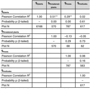
of plant species in both are similar, broad-leafed forests show higher numbers of moss and mollusk species than artificial meadows do. A correlation analysis was done between plant species, threatened plant species, moss and mollusks species (Table 3). The results reveal a relatively clear and highly significant correlation between the number of all plant spe-cies and the number of threatened spespe-cies. The correlation between the number of plant species and the number of moss species is less clear, but still significant.
2.3 β-Diversity
The slope parameter z of the fitted power function was taken as an indicator of β-diversity. The rarefaction curves are based
on 39 sample plots for each of six land use types (Fig. 3). The fitted curve parameter z for vascular plants reveal no differences between land use types (Table 4). For mollusk species, however, β-diversity – and thus, species turnover – is different between land use types. The β-diversity of mol-lusks is generally low for forests and high for arable land, grassland and bare rock.
2.4 Ecosystem damage potential on the local scale EDPS
The basis for calculating the local damage is the species num-ber (α-diversity) of a specific land use type Socc standardized for 1 m2.β-Diversity was not included in the
characteriza-tion factor, because not enough sample plots were available for reliably estimating parameters.
Table 2: Standardized species numbers S (vascular plants, moss, mollusks) for specific land use types, intensity classes, and Swiss regions. The area
chosen for standardization was 1 m2. Calculated for Switzerland on the basis of the BDM data set, there are 1061 vascular species, 519 moss species, and 133 mollusk species (cont'd)
Splants Sthreatened plants Smoss Smollusks
C O RINE Pl u s I D Me a n Std . E rr o r Mi ni m u m Me d ia n Ma x im u m N P lo ts Me a n Std . E rr o r N P lo ts Me a n Std . E rr o r N P lo ts Me a n Std . E rr o r N P lo ts 313 Mixed forest 9.9 0.6 1 8 28 83 0 5.7 0.4 35 7.3 0.7 36 " above 800m 19.3 0.5 3 19 36 223 0 9.0 0.6 46 5.7 0.5 46 313a Mixed broad-leafed forest 12.6 1.1 9 14 18 8 0 0 0 313b Mixed coniferous forest 7.1 0.3 5 7 11 35 0 6.9 1.2 2 3.1 0.0 2 313c Mixed plantations 4.3 0.3 2 4 11 61 0 0 0 314 Forest Edge 18.5 1.1 1 18 40 78 0 0 0 321 Semi-natural grassland 18.3 0.5 2 17 49 331 0.7 0.0 19 9.2 0.6 86 3.3 0.3 66 322 Moors and heath land 14.2 1.1 5 13 29 36 0.9 0.3 2 11.1 0.9 30 3.4 0.8 21 324 Transitional woodland/shrub 17.2 1.0 2 18 34 60 0.6 0.0 2 10.3 1.5 16 4.7 1.0 13 331 Beaches, dunes, and sand
plains
5.6 2.5 3 6 8 2 0 1.6 0.9 2 1.9 – 1 332 Bare rock 8.7 0.9 1 7 22 42 1.2 1 6.9 0.6 40 1.9 0.4 18 333 Sparsely vegetated areas 19.8 1.4 5 20 42 31 0.6 0.0 6 11.4 1.0 30 2.4 0.6 23 411 Inland marshes 18.0 3.7 9 16 28 5 1.0 0.2 3 4.1 1.6 5 9.4 2.3 5 412 Peat bogs 7.2 0.2 1 7 24 634 0 3.1 – 1 4.4 – 1 511 Water courses 7.5 2.6 2 7 16 5 0.6 1 4.9 1.2 5 1.7 0.7 3 Total 11.8 0.1 0 10 49 5581 0.7 0.0 78 6.1 0.2 787 4.2 0.1 617 Intensity classes 1 Artificial surfaces 9.4 0.3 0 9 37 481 0.6 0.0 7 3.9 0.4 38 4.3 0.6 31 2 Agriculture high intensity 5.8 0.2 0 5 30 524 0.7 0.1 11 1.6 0.1 47 2.9 0.3 58 2 Agriculture low intensity 16.6 0.2 2 16 49 1214 0.7 0.0 19 9.1 0.6 89 3.3 0.3 70 3 Forestry high intensity 5.7 0.2 1 5 18 140 0 5.8 0.7 6 3.9 0.4 6 3 Forestry low intensity 11.0 0.2 1 9 36 1773 0 3.9 0.3 200 6.3 0.4 86 3 Non-use 11.1 0.2 1 10 42 1120 0.8 0.1 15 9.2 0.5 125 3.4 0.4 83 Regions in Switzerland Alps 19.7 0.2 12 19 33 202 0.7 0.0 172 0 0 Jura 17.1 0.4 12 18 23 44 0.7 0.1 33 0 0 Plateau 15.6 0.3 11 15 24 104 0.1 0.0 23 0 0 Above timberline 10.7 0.2 3 10 22 215 0.2 0.0 177 0 0 Lakes 0.5 0.1 0 0 1 28 1.0 0.1 87 0 0
Worldwide diversity regions
DZ5 (Swiss Plateau) 8.9 13.3 DZ6 (Swiss Alps) 13.3 17.7
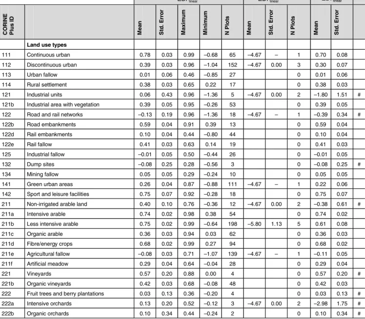
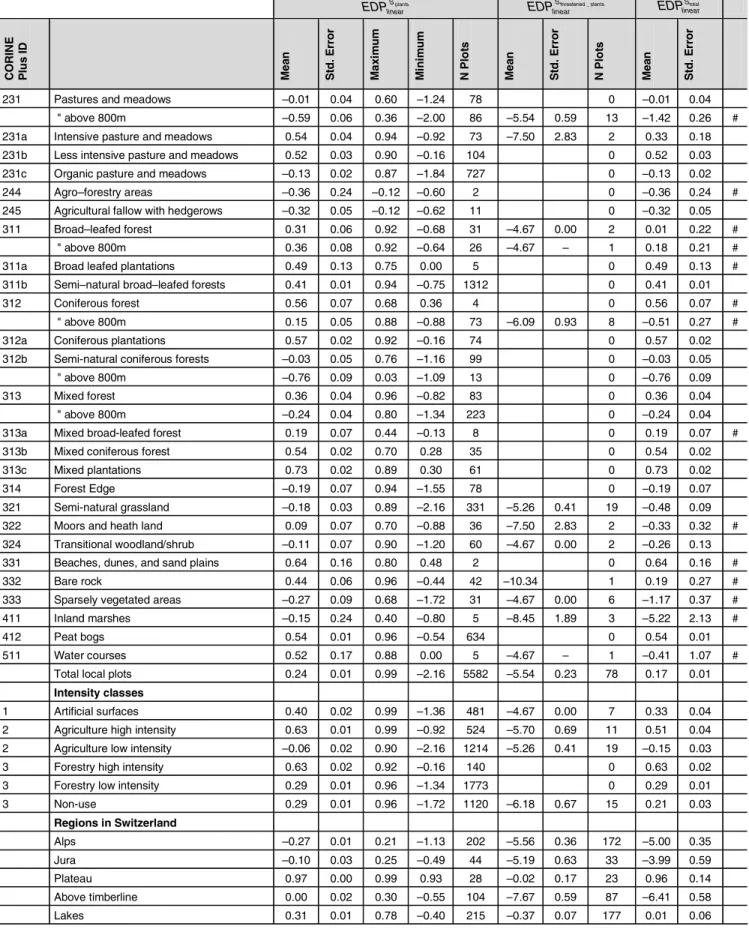
Linear transformations of the relative species numbers re-sult in ecosystem damage potentials ( EDPlinearS , Table 5). The
integration of threatened plant species diversity into EDPlinearStotal
makes it possible to differentiate between land use types that have similar total species numbers, but intensities of land use that are clearly different (e.g. artificial meadow and broad-leafed forest). Negative impact values indicate that land use types hold more species per m2 than the reference does. In
terms of species diversity, these land use types are superior. In Table 5 EDPlinearStotal, with a few number of plots – and therefore,
high standard error – are flagged with #.
The nonlinear transformation resulting in EDPnonlinearStotal is shown
in Table 6. Since α-diversity of plants, moss and mollusks is uncorrelated or correlated with low R2(see Table 3), rankings
of land use types are different according to whether they are based on EDPnonlinearSplants , EDP
nonlinear
Smoos or EDP nonlinear
Smollusks .
Although the type of transformation and species groups in-cluded differ, EDPlinearStotal and EDP
nonlinear
Stotal values for intensity
classes are very similar. Remarkable differences have values for low intensity forests. This is explained by the fact that those forests have a rather low α-diversity of threatened plants and, because of their humid habitat conditions, a high α-diversity of moss and mollusks.
Splants Sthreatened plants Smoss Smollusks Splants Pearson Correlation R2 1.00 0.51** 0.29** 0.02 Probability p (2-tailed) – 0.00 0.00 0.61 Plot N 6166 570 787 617 Sthreatened plants Pearson Correlation R2 1.00 –0.13 –0.05 Probability p (2-tailed) – 0.29 0.73 Plot N 570 68 62 Smoss Pearson Correlation R2 1.00 0.06 Probability p (2-tailed) – 0.16 Plot N 787 563 Smollusks Pearson Correlation R2 1.00 Probability p (2-tailed) – Plot N 617
** Correlation is significant at the p=0.01 level (2-tailed)
Table 3: Correlation of species groups
Land-use type CORINE Plus ID Plants Mollusks
c z c z
Less intensive arable (≤800m) 2112 2.39 0.78 0.44 0.68 Pastures and meadows (>800m) 231 2.49 0.78 0.90 0.61
Pastures and meadows (≤800m) 231 1.91 0.78 0.47 0.52 Coniferous forest (>800m) 312 2.21 0.78 0.71 0.55 Mixed forest (>800m) 313 2.37 0.81 0.36 0.51 Mixed forest (≤800m) 313 2.47 0.79 0.25 0.45 Semi-natural grassland (>800m) 321 2.12 0.80 0.48 0.72 Bare rock (>800m) 332 2.20 0.79 0.11 0.83
Table 4: Curve parameter for the power function E(S)=cAz fitted to a discontinuous rarefaction function. A distinction is made between land use types
below 800 m above sea level and above
Table 5: Local ecosystem damage potential based on total plant species data and data on threatened plant species (EDPlinear
S ). Means and standard error
are calculated according to the linear function (equation [6]) with the Swiss Plateau as reference. EDPlinear
S values are dimensionless, but refer to 1 m2 of specific land use types, intensity classes and the Swiss regions. Uncertain values of EDPlinear
Stotal with standard error above 0.2 are flagged with #. Those are
not recommended for use in LCIA
€ EDPlinear Splants € EDPlinear Sthreatened _ plants € EDPlinear Stotal CO R IN E Pl u s I D Me a n St d . E rr o r Ma x im u m Min im u m N P lo ts Me a n St d . E rr o r N P lo ts Me a n St d . E rr o r
Land use types
111 Continuous urban 0.78 0.03 0.99 –0.68 65 –4.67 – 1 0.70 0.08 112 Discontinuous urban 0.39 0.03 0.96 –1.04 152 –4.67 0.00 3 0.30 0.07 113 Urban fallow 0.01 0.06 0.46 –0.85 27 0 0.01 0.06 114 Rural settlement 0.38 0.03 0.65 0.22 17 0 0.38 0.03 121 Industrial units 0.06 0.43 0.96 –1.36 5 –4.67 0.00 2 –1.80 1.51 # 121b Industrial area with vegetation 0.39 0.05 0.95 –0.26 53 0 0.39 0.05 122 Road and rail networks –0.13 0.19 0.96 –1.36 18 –4.67 – 1 –0.39 0.34 # 122b Road embankments 0.59 0.04 0.91 0.39 13 0 0.59 0.04 122d Rail embankments 0.10 0.04 0.44 –0.80 44 0 0.10 0.04 122e Rail fallow 0.41 0.03 0.63 0.14 19 0 0.41 0.03 125 Industrial fallow –0.01 0.05 0.50 –0.44 26 0 –0.01 0.05 132 Dump sites –0.08 0.25 0.28 –0.56 3 0 –0.08 0.25 # 134 Mining fallow 0.05 0.05 0.29 –0.24 10 0 0.05 0.05 141 Green urban areas 0.26 0.04 0.87 –0.88 111 –4.67 – 1 0.22 0.06 142 Sport and leisure facilities 0.75 0.07 0.92 –0.28 18 0 0.75 0.07 211 Non-irrigated arable land 0.40 0.10 0.76 –0.36 12 –4.67 0.00 2 –0.38 0.61 # 211a Intensive arable 0.74 0.02 0.98 0.38 54 0 0.74 0.02 211b Less intensive arable 0.75 0.02 0.99 –0.64 198 –5.80 1.13 5 0.61 0.08 211c Organic arable 0.36 0.03 0.94 0.03 62 0 0.36 0.03 211d Fibre/energy crops 0.68 0.02 0.99 0.27 94 0 0.68 0.02 211e Agricultural fallow –0.08 0.03 0.71 –1.07 139 –4.67 – 1 –0.11 0.05 211f Artificial meadow 0.29 0.04 0.64 –0.04 28 0 0.29 0.04 221 Vineyards 0.57 0.20 0.88 0.00 4 0 0.57 0.20 # 221b Organic vineyards 0.42 0.03 0.68 –0.08 48 0 0.42 0.03 222 Fruit trees and berry plantations 0.03 0.13 0.36 –0.20 4 0 0.03 0.13 # 222a Intensive orchards 0.13 0.20 0.52 –0.12 3 –4.67 0.00 2 –2.98 1.75 # 222b Organic orchards 0.10 0.34 0.44 –0.24 2 0 0.10 0.34 #
Table 5: Local ecosystem damage potential based on total plant species data and data on threatened plant species (EDPlinear
S ). Means and standard error
are calculated according to the linear function (equation [6]) with the Swiss Plateau as reference. EDPlinear
S values are dimensionless, but refer to 1 m2 of specific land use types, intensity classes and the Swiss regions. Uncertain values of EDPlinear
Stotal with standard error above 0.2 are flagged with #. Those are
not recommended for use in LCIA (cont'd)
€
EDPlinearSplants
€ EDPlinear Sthreatened _ plants € EDPlinear Stotal CO RIN E Pl u s I D Me a n St d . Er ro r Ma x im u m Mi n im u m N P lo ts Me a n St d . Er ro r N P lo ts Me a n St d . Er ro r
231 Pastures and meadows –0.01 0.04 0.60 –1.24 78 0 –0.01 0.04 " above 800m –0.59 0.06 0.36 –2.00 86 –5.54 0.59 13 –1.42 0.26 # 231a Intensive pasture and meadows 0.54 0.04 0.94 –0.92 73 –7.50 2.83 2 0.33 0.18 231b Less intensive pasture and meadows 0.52 0.03 0.90 –0.16 104 0 0.52 0.03 231c Organic pasture and meadows –0.13 0.02 0.87 –1.84 727 0 –0.13 0.02
244 Agro–forestry areas –0.36 0.24 –0.12 –0.60 2 0 –0.36 0.24 # 245 Agricultural fallow with hedgerows –0.32 0.05 –0.12 –0.62 11 0 –0.32 0.05 311 Broad–leafed forest 0.31 0.06 0.92 –0.68 31 –4.67 0.00 2 0.01 0.22 #
" above 800m 0.36 0.08 0.92 –0.64 26 –4.67 – 1 0.18 0.21 # 311a Broad leafed plantations 0.49 0.13 0.75 0.00 5 0 0.49 0.13 # 311b Semi–natural broad–leafed forests 0.41 0.01 0.94 –0.75 1312 0 0.41 0.01 312 Coniferous forest 0.56 0.07 0.68 0.36 4 0 0.56 0.07 #
" above 800m 0.15 0.05 0.88 –0.88 73 –6.09 0.93 8 –0.51 0.27 # 312a Coniferous plantations 0.57 0.02 0.92 –0.16 74 0 0.57 0.02 312b Semi-natural coniferous forests –0.03 0.05 0.76 –1.16 99 0 –0.03 0.05
" above 800m –0.76 0.09 0.03 –1.09 13 0 –0.76 0.09 313 Mixed forest 0.36 0.04 0.96 –0.82 83 0 0.36 0.04
" above 800m –0.24 0.04 0.80 –1.34 223 0 –0.24 0.04 313a Mixed broad-leafed forest 0.19 0.07 0.44 –0.13 8 0 0.19 0.07 # 313b Mixed coniferous forest 0.54 0.02 0.70 0.28 35 0 0.54 0.02 313c Mixed plantations 0.73 0.02 0.89 0.30 61 0 0.73 0.02 314 Forest Edge –0.19 0.07 0.94 –1.55 78 0 –0.19 0.07 321 Semi-natural grassland –0.18 0.03 0.89 –2.16 331 –5.26 0.41 19 –0.48 0.09 322 Moors and heath land 0.09 0.07 0.70 –0.88 36 –7.50 2.83 2 –0.33 0.32 # 324 Transitional woodland/shrub –0.11 0.07 0.90 –1.20 60 –4.67 0.00 2 –0.26 0.13 331 Beaches, dunes, and sand plains 0.64 0.16 0.80 0.48 2 0 0.64 0.16 # 332 Bare rock 0.44 0.06 0.96 –0.44 42 –10.34 1 0.19 0.27 # 333 Sparsely vegetated areas –0.27 0.09 0.68 –1.72 31 –4.67 0.00 6 –1.17 0.37 # 411 Inland marshes –0.15 0.24 0.40 –0.80 5 –8.45 1.89 3 –5.22 2.13 # 412 Peat bogs 0.54 0.01 0.96 –0.54 634 0 0.54 0.01 511 Water courses 0.52 0.17 0.88 0.00 5 –4.67 – 1 –0.41 1.07 #
Total local plots 0.24 0.01 0.99 –2.16 5582 –5.54 0.23 78 0.17 0.01
Intensity classes
1 Artificial surfaces 0.40 0.02 0.99 –1.36 481 –4.67 0.00 7 0.33 0.04 2 Agriculture high intensity 0.63 0.01 0.99 –0.92 524 –5.70 0.69 11 0.51 0.04 2 Agriculture low intensity –0.06 0.02 0.90 –2.16 1214 –5.26 0.41 19 –0.15 0.03 3 Forestry high intensity 0.63 0.02 0.92 –0.16 140 0 0.63 0.02 3 Forestry low intensity 0.29 0.01 0.96 –1.34 1773 0 0.29 0.01 3 Non-use 0.29 0.01 0.96 –1.72 1120 –6.18 0.67 15 0.21 0.03 Regions in Switzerland Alps –0.27 0.01 0.21 –1.13 202 –5.56 0.36 172 –5.00 0.35 Jura –0.10 0.03 0.25 –0.49 44 –5.19 0.63 33 –3.99 0.59 Plateau 0.97 0.00 0.99 0.93 28 –0.02 0.17 23 0.96 0.14 Above timberline 0.00 0.02 0.30 –0.55 104 –7.67 0.59 87 –6.41 0.58 Lakes 0.31 0.01 0.78 –0.40 215 –0.37 0.07 177 0.01 0.06
€
EDPnonlinearSplants
€
EDPnonlinearSmoos
€
EDPnonlinearSmollusk
€
EDPnonlinearStotal
CO R INE Pl u s I D Me a n Std . E rr o r N P lot s Me a n Std . E rr o r N P lot s Me a n Std . E rr o r N P lot s Me a n Std . E rr o r N P lot s
Land use type
111 Continuous urban 0.24 0.10 5 0.42 0.06 5 –0.10 0.19 3 0.59 0.18 5 # 112 Discontinuous urban 0.10 0.05 25 0.25 0.04 23 –0.01 0.04 20 0.32 0.08 25 121 Industrial units 0.14 0.25 4 0.32 0.10 4 0.13 0.16 3 0.56 0.34 4 # 122 Road and rail networks 0.08 0.10 13 0.22 0.06 12 –0.10 0.07 11 0.20 0.16 13
132 Dump sites –0.01 0.06 3 0.30 0.06 3 0.35 0.10 3 0.65 0.19 3 # 141 Green urban areas –0.17 – 1 0.08 – 1 –0.17 – 1 –0.27 – 1 # 142 Sport and leisure facilities 0.07 0.13 2 0.44 0.28 2 –0.33 – 1 0.34 0.58 2 # 211 Non–irrigated arable land 0.22 0.04 8 0.48 0.07 5 0.23 0.07 5 0.66 0.12 8 # 211b Less intensive arable 0.20 0.03 30 0.61 0.04 15 0.14 0.04 24 0.62 0.07 30 211e Agricultural fallow –0.14 1 0.20 – 1 0.15 – 1 0.21 – 1 # 211f Artificial meadow 0.10 0.01 26 0.48 0.03 22 0.06 0.04 23 0.56 0.06 26 221 Vineyards 0.31 0.12 4 0.72 1 –0.06 0.09 4 0.43 0.15 4 # 222 Fruit trees and berry plantations 0.02 0.04 4 0.52 0.15 4 –0.07 0.03 4 0.47 0.09 4 # 222a Intensive orchards 0.06 0.07 3 0.44 0.09 2 0.00 0.09 3 0.35 0.20 3 # 222b Organic orchards 0.05 0.11 2 0.72 – 1 –0.05 0.12 2 0.36 0.59 2 # 231 Pastures and meadows 0.02 0.01 74 0.48 0.03 60 0.03 0.03 72 0.43 0.04 74 " above 800m –0.11 0.01 73 0.22 0.03 69 0.08 0.03 70 0.18 0.05 73 231a Intensive pasture and meadows –0.10 0.07 3 0.36 0.06 3 0.04 0.12 3 0.31 0.13 3 # 244 Agro-forestry areas –0.08 0.05 2 –0.01 0.14 2 0.08 0.07 2 0.00 0.26 2 # 311 Broad-leafed forest 0.13 0.03 30 0.09 0.03 30 –0.18 0.04 29 0.06 0.06 30 " above 800m 0.19 0.04 25 0.11 0.04 25 0.03 0.06 21 0.33 0.10 25 311b Semi-natural broad-leafed forests 0.04 0.01 115 0.61 0.02 115 – – 0 0.65 0.02 115 312 Coniferous forest 0.27 0.03 3 0.00 0.08 3 –0.13 0.11 3 0.14 0.16 3 # " above 800m 0.09 0.02 73 0.00 0.02 73 0.06 0.03 66 0.15 0.04 73 312a Coniferous plantations 0.22 0.10 6 0.14 0.04 6 –0.04 0.03 6 0.31 0.15 6 # 312b Semi-natural coniferous forests 0.09 0.30 2 0.00 0.01 2 –0.09 0.05 2 0.00 0.23 2 # 313 Mixed forest 0.19 0.03 36 0.15 0.02 35 –0.16 0.03 36 0.17 0.05 36
" above 800m 0.12 0.02 47 0.03 0.02 46 –0.07 0.04 46 0.09 0.06 47
313b Mixed coniferous forest 0.15 0.05 2 0.08 0.05 2 0.02 0.00 2 0.25 0.00 2 # 321 Semi-natural grassland –0.13 0.01 88 0.05 0.02 86 0.09 0.03 66 –0.01 0.03 88 322 Moors and heath land 0.02 0.02 30 –0.03 0.02 30 0.11 0.06 21 0.07 0.06 30 324 Transitional woodland/shrub –0.01 0.03 16 0.02 0.05 16 –0.02 0.06 13 0.00 0.08 16 331 Beaches, dunes, and sand plains 0.31 0.13 2 0.54 0.19 2 0.15 – 1 0.92 0.39 2 # 332 Bare rock 0.23 0.03 41 0.13 0.03 40 0.23 0.05 18 0.45 0.06 41 333 Sparsely vegetated areas –0.04 0.02 31 –0.02 0.03 30 0.19 0.05 23 0.08 0.06 31 411 Inland marshes –0.01 0.06 5 0.29 0.10 5 –0.23 0.10 5 0.05 0.13 5 # 412 Peat bogs 0.05 – 1 0.29 – 1 –0.08 – 1 0.26 – 1 # 511 Water courses 0.28 0.11 5 0.20 0.07 5 0.24 0.13 3 0.63 0.16 5 #
Intensity class
1 Artificial surfaces 0.11 0.04 40 0.29 0.03 38 0.01 0.04 31 0.39 0.07 40 2 Agriculture high intensity 0.15 0.02 70 0.51 0.02 47 0.11 0.03 58 0.58 0.04 70 2 Agriculture low intensity –0.13 0.01 92 0.06 0.02 89 0.09 0.03 70 –0.01 0.03 92
3 Forestry high intensity 0.22 0.10 6 0.14 0.04 6 –0.04 0.03 6 0.31 0.15 6 # 3 Forestry low intensity 0.09 0.01 202 0.39 0.02 200 –0.11 0.02 86 0.43 0.03 202 3 Non-use 0.07 0.02 127 0.06 0.02 125 0.12 0.03 83 0.20 0.04 127
Table 6: Local ecosystem damage potential based on data on plant, moss and mollusk species (EDPnonlinear
S ). For their calculation, the non-linear model
was used according to equation [8]. They are dimensionless, but refer to 1 m2 of land. Uncertain values of EDP
nonlinear
Stotal with low number of sample plots n
2.5 Use of characterization factors EDPS for calculation of damages for land occupation and land use change In this section, we explain how to use the characterization factors EDPSin Life Cycle Impact Assessment. For calcula-tion of the damage of land occupacalcula-tion, we refer to equacalcula-tion (2) of Part 1 of Koellner and Scholz (2007). For a specific land use type the time of occupation in years is multiplied with the area in m2 and also multiplied with the EDP factor
for this specific land use type. We recommend using linear
EDPlinearStotal from Table 5. They are more robust compared to
the nonlinear version.
More difficult is the situation when calculating the damage
of land use change. We argued in Section 3.3 of Part 1 that
land use change includes damage from transformation and restoration. The damage for transformation and restora-tion are calculated according to equarestora-tions (5) and (6) (Koellner and Scholz 2007). Taking, for example, the land use change from low intensity forest into high intensity ag-riculture, the damage is without taking the baseline dam-age into account:
(9)
Assuming that Achange = Atrans = Arest and with EDPagri_hi = 0.51 and EDPforest_li = 0.29 from Table 5, and with Tforest_li – > agri_hi = 1, Tagri_hi –> forest_li = 50 from Table 2 (Part 1 of this paper series) it is
(10)
In this example, the phase of transformation from forest into agriculture accounts for less damage than the phase of the restoration of the forest. The main reason for the differ-ence is the long restoration time in relation to transforma-tion time. For practical applicatransforma-tions, the damage of the trans-formation phase could be neglected, if transtrans-formation is rapid compared to restoration. The damage of changing 1 unit area from low intensity forest to high intensity agriculture is more then ten times higher compared to the occupation of 1 unit area of existing high intensity agriculture for 1 year (Docc = Aocc · Tocc · EDPagri_hi = Aocc · 1 · 0.51). This example shows that it makes sense to maximize occupation time of existing high intensity agriculture and minimize transforma-tion of forest into agricultural land use to achieve constant functional output.
3 Discussion
3.1 Validity of ecosystem damage potential EDPS
Land use has severe impacts, not only on biodiversity, but also on ecosystem services (e.g. water purification, carbon sequestration, biomass productivity) and scenic beauty (Daily 1997). A comprehensive assessment of the ecosystem dam-age potential of land use requires the integration of all those aspects. We focused on biodiversity, because it is an impor-tant aspect of the ecosystem. Biodiversity is regarded as a key element for ecosystem functioning (Naeem and Li 1997, Schläpfer and Schmid 1999, Schulze and Mooney 1994) and its intrinsic value is stressed by the Convention on Biologi-cal Diversity (UNEP 1992).
The ecosystem damage potential EDPS is based on assess-ment of impacts of land use on species diversity. We clearly base EDPSfactors on α-diversity, which correlates with the local aspect of species diversity of land use types. Based on an extensive meta-analysis of biologists' field research, we were able to include data on the diversity of plant species, threatened plant species, moss and mollusks in the EDPS. The integration of other animal species groups (e.g. insects, birds, mammals, amphibians) with their specific habitat pref-erences could change the characterization factors values spe-cific for each land use type. Ecosystem functions are sup-ported by those mobile species groups, because they provide functional links between habitats in the landscape (Lundberg and Moberg 2003). Many studies propose characterization factors based on α-diversity. More specifically these focus either on species lost or absolute number of species on the local scale. Factors proposed are potentially disappeared frac-tion of vascular plant species (Goedkoop et al. 1998, Goed-koop and Spriensma 1999) or loss of vascular plant species per area (Udo de Haes et al. 1999), Other propose to take the number of species separated into different groups, i.e. tree, shrub, and herb species (Schweinle 1998), diversity of trees and structural diversity of forest (Giegrich and Sturm 1996) or number of rare species and number of all species (Cowell 1998). We propose also a relative indicator for
α
-diversity, because absolute numbers of local species diver-sity generally increase from South to North, even for the same type of land use type.In addition β-diversity is an important aspect of species di-versity, because not only absolute or relative species num-bers, but similarities of species composition between differ-ent plots of one land use types are compared. Lindeijer et al. (1998) proposed to take species accumulation rate per land use type as an indicator. Changes are assessed on a cardinal scale for different ecosystems worldwide. Koellner (2004) gives examples of an indicator for β-diversity for different functional species groups, which are somehow, linked to different land use types (e.g., forest species, unfertilized meadow species, fertilized meadow species). There was a large difference found between the functional species groups, however, data are not sufficient to derive characterization factors for LCA, because the link to specific land use types is not clear enough. In contrast the factors calculated in this paper (see Table 4) are directly linked to specific land use types, but results are ambiguous, mainly because of data
limitations, which are expected to less severe in the future. For this reasons β-diversity could not be included in the cal-culation of EDPS in this paper,
Vogtländer (2004) proposed characterization factors based on the diversity of ecosystems and Müller-Wenk (1998) on the occurrence of rare ecosystems on the landscape scale. In our assessment, this has been integrated indirectly, because we took the number of threatened plant species into account. Generally speaking, species which are bound to scarce eco-system types are rare on the landscape scale. Semi-natural grassland, moors, heath land and inland marshes are such rare ecosystem types and show high number of threatened species. These ecosystem types have severely lost areas in the course of the development of industrial agriculture, in-tensive forestry and urban areas sprawl.
Such characterization factors refer to γ-diversity and to the assessment of regional impacts of land use. A proposal how to assess regional land use impacts based on a regression analy-sis with species potentially lost between about 1850 and 1975 (dependent variable) and land use on the regional scale (inde-pendent variable) was given by Koellner (2003). Although the quality of the available data was high, the results were not very robust and limited to the specific regional charac-teristics of Switzerland. But again, with better data availabil-ity in the future, it will be possible to calculate characteriza-tion factors based also on this aspect of biodiversity. The linear transformation of species data into EDPlinearStotal
as-signs the same value to each plant species and allows for accounting the non-use value of species diversity. For the same reason, we also integrated the number of threatened species separately. Since data on moss and mollusks diver-sity was only available for a sub-sample (841 out of 5,581 plots), it was not included here. The nonlinear
transforma-tion into EDPnonlinearStotal was developed to account for the
func-tional aspect of species diversity. According to the redun-dant species hypothesis, the relationship between species loss and ecosystem functioning is nonlinear. The reasoning be-hind this hypothesis is that species are redundant, as dem-onstrated by the fact that a specific ecological function (e.g. fixation of nitrogen) can be fulfilled by different species (Lawton 1996). The assumption underlying this is that all of the species within one functional group are equally adapted for fulfilling the same specific function (Schulze and Mooney 1994, pp. 501), but in fact, species within one functional group differ, particularly in their response to environmental changes. Formerly, redundant species might become impor-tant for ecosystem functioning, because they are better adapted to new environmental conditions. This point is very much stressed in the rivet hypothesis, framed by Ehrlich and Ehrlich (1981).
The empirical data used for the development of EDPS were acquired from Switzerland and Germany. The external va-lidity refers to the question of whether EDPScan be gener-alized to other regions or countries. Most of the data was sampled from regions which were subject to intensive use and consist largely of agriculture, forestry, and urban land. One can expect that the absolute species number will be
valid for regions which are similar in land use intensity and biogeographical situation. We used a relative measure for lo-cal species richness and took the regional species richness as a reference. As a result, the error might be less significant when the findings are generalized to other European countries. The coarse ranking of the land use types is expected to be stable across a wide geographical range. The calculated EDPS are expected to be valid for the European part of diversity zones 5 and 6 of Barthlott's (1999) map of global diversity.
Limitation of the approach is that a land use is only speci-fied in terms of type, area and duration. Specific character-istics of patch size and shape, location of patches in the land-scape and their fragmentation have large impacts on abundance and diversity of species (Fahrig and Jonsen 1998). Due to data limitations, all those factors could not be in-cluded in this assessment.
One issue pertaining to internal validity is whether calcu-lated factors only refer to land use impacts or also refer to other impacts. In the latter case, double counting of impacts would occur, since some other impact categories (e.g. nutrification and ecotoxicological effects) are assessed sepa-rately in LCIA. In contrast to the suggestions of Udo de Haes (2006) and Milà i Canals et al. (2007), the characterization factors for land use calculated in this paper integrate all the impacts which result from land use. These impacts include the intentional application of chemicals, such as in agricul-ture, where fertilizer and pesticides are used, as well as physi-cal impacts like ploughing. If one wants to include damage to biodiversity in LCIA, it is not possible to separate those chemical and physical impacts. However, it is necessary to distinguish (i) impacts on the plot of land use from (ii) im-pacts outside of this immediate plot resulting from runoff. In the former case, both the physical and chemical impacts of land use are included in the characterization factor EDPS. However, in the latter case, damage due to impacts from runoff are not included in the EDPS factor, but must be con-sidered in other impact categories. One can conclude from this that double counting is not a problem, when local EDPS factors are used, which refer only to the plot in use. How-ever, if regional factors referring to γ-diversity could be cal-culated, double counting would be a problem to be addressed. 3.2 Uncertainty of characterization factors EDPS
In EDPS, the uncertainty of the results is strongly influenced by the empirical data basis of the species diversity. An im-portant source of uncertainty in meta-analysis is the reli-ability. This refers to the stability of results when many re-searchers have conducted the investigations or different methods have been used. In our meta-analysis on species diversity, we took 23 different sources into account. The data for species diversity was mostly sampled according to the standardized method from Braun-Blanquet, which is applied in vegetation science, although other methods were also used to determine species richness. The accuracy of data can also vary from researcher to researcher, but it is difficult to judge this aspect of reliability on the basis of the available literature. The data on plant moss and mollusk species for the 841 plots from the Biodiversity Monitoring Switzerland are highly reliable.