A-infinity algebras for Lagrangians via polyfold theory for Morse trees with holomorphic disks

(1)

A-infinity algebras for Lagrangians via polyfold theory for

Morse trees with holomorphic disks

by

Jiayong Li

Submitted to the Department of Mathematics in partial fulfillment of the requirements for the degree of

Doctor of Philosophy at the

MASSACHUSETTS INSTITUTE OF TECHNOLOGY

DEC

2 4 2015

LIBRARIES

September 2015

The author hereby grants to MIT permission to reproduce and to distribute publicly paper and electronic copies of this thesis document in whole or in part in any

medium now known or hereafter created.

Signature redacted

Author... ... ;.. .........................

Department of Mathematics August 7, 2015

Certified by...

Signature redacted

...

Katrin Wehrheim Professor Thesis Supervisor

Accepted by ...

Signature redacted...

Alexei Borodin Chairman, Department Committee on Graduate Theses

(2)

(3)

A-infinity algebras for Lagrangians via polyfold theory for Morse trees with holomorphic disks

by Jiayong Li

Submitted to the Department of Mathematics on August 7, 2015, in partial fulfillment of the

requirements for the degree of Doctor of Philosophy

Abstract

For a Lagrangian submanifold, we define a moduli space of trees of holomorphic disk maps with Morse flow lines as edges, and construct an ambient space around it which we call the quotient space of disk trees. We show that this ambient space is an M-polyfold with boundary and corners by combining the infinite dimensional analysis in sc-Banach space with the finite dimensional analysis in Deligne-Mumford space. We then show that the Cauchy-Riemann section is sc-Fredholm, and by applying the polyfold perturbation we construct an A.. algebra over Z2 coefficients. Under certain assumptions, we prove the invariance of this algebra with respect to choices of almost-complex structures.

Thesis Supervisor: Katrin Wehrheim Title: Professor

(4)

(5)

Acknowledgments

I am grateful to my advisor Katrin Wehrheim for her patience, generosity, and mathematical wisdom. I would like to thank Yael Karshon, Nate Bottman, Michael Hutchings, Helmut Hofer, Tom Mrowka, Paul Seidel, and Jo Nelson for many helpful discussions. My gratitude goes out to the wonderful staff members Barbara Peskin and Janka Moss. I am also grateful for the camaraderie of John Binder, Roberto Svaldi, Michael Donovan, Dana Mendelson, Michael Andrews, Saul Glasman, Jan-Christian Huetter, Zihan Liu, Steve Voinea, Louis Perna, and Rohan Padhye. Lastly, I would like to thank my mom and dad for their love and support.

(6)

(7)

9M.

. 7.2.1 Proof of Theorem 7.22 . . . . 7.2.2 Proof of Theorem 7.21 . . . . 8 Proof for the Topology and the Atlas of the Quotient

8.1 Sc-smoothness of Splicing . . . . 8.2 Closedness of the Biholomorphic Equivalence in X . . 8.2.1 Proof of Theorem 8.4 . . . .

8.2.2 Continuity and Sc-smoothness of Glued Maps i

8.2.3 Stabilization Revisited . . . . 8.3 Openness of the Biholomorphic Equivalence in X . . . 9 Oj the Cauchy-Riemann Section

9.1 T) the Bundle of Complex Anti-linear Sections . . . . 9.2 Sc-smoothness of Oj the Cauchy-Riemann Section . . . . 9.3 Filled Section of Oj and the Polyfold redholm Property . . . 10 Transversality with Boundary and Corners in M-polyfolds

11 A, Algebra and Concatenation Tree

11.1 Curved A, Algebra . . . . 11.2 Type and Disk Tree A, Algebra . . . . 11.3 Concatenation . . . . 11.4 Concatenation and the Boundary and Corners Structure . . .

75 83 . . . . 83 . . . . 84 . . . . 88 . . . . 93 . . . . 102 . . . . 106 . . . . 112 . . . . 134 Space of Disk 1 Standard Mod( Trees139 . . . 139 . . . 145 . . . 149 1 . . 155 . . . 157 . . . 160 179 . . . 179 . . . 183 . . . 187 189 195 . . . 195 . . . 197 . . . 199 . . . 202

(9)

11.5 Compatible Section and A,, Algebra . . . .2 11.6 Gluing Near Boundary and Corners . . . .

12 Independence of the Almost-Complex Structures 12.1 Index -1 and Index (-1, 0) Concatenation Trees . . 12.2 Transversality of 1-family of Sc-Fredholm Sections 12.3 A,, Isomorphism Across Accident Times . . . . 12.4 1-Parameter Gluing Problem . . . . 12.5 Proof of A,, Isomorphism . . . .

13 Appendix

13.1 Disk Automorphism . . . . 13.2 Exponential and Logarithm Gluing Profiles . . . . 13.3 Sc-smoothness Results . . . . . . . . 207 211 . . . . 2 12 . . . . 2 13 . . . . 2 16 . . . . 2 17 . . . . 22 1 237 . . . . 237 . . . . 24 1 . . . . 248 . . . . 204

(10)

(11)

Chapter 1 Introduction

This introduction gives an informal description of the main objects and a quick survey of the main results. Let (M, w) be a symplectic manifold of dimension 2n with wl,(iM) = 0, and L a Lagrangian submanifold of M. In addition, we choose a compatible almost complex structure J on M, and a Morse-Smale pair (f, g) on the Lagrangian L. We denote by D the closed unit disk in C.

Let pk,... ,pi, q be Morse critical points of

f,

p an integer, and v a non-negative real

number. The moduli space of holomorphic disk trees 9R([pk ®... Opi, q; M], v) consists

of equivalence classes of the form [T, -y, x, u]. Here T is an ordered tree with edges E and vertices V. Since the tree is ordered, each edge has a direction. Hence we view E as a subset of (V x V) \ A, and each edge is of the form e = (v-, v+). Furthermore, the set of vertices V is partitioned into main vertices and critical vertices V = Vm LJ VC. The set of critical

vertices V' contains k leaf vertices wk, ... , wi, and the root vertex rt(T), which correspond to the critical points Pk, . . , p1, and q, respectively. The tuple -/ consists of generalized Morse trajectories -y for each edge e E E. (A generalized Morse trajectory can be a series of broken Morse flow lines. See [20] for a thorough exposition and Section 2.2 for a brief description.) The tuple (x, u) consists of boundary marked points and J-holomorphic disk maps (!v, uv) for each main vertex v C Vm. More precisely, Kv = {Xv,e E D Ie adjacent to v} is an

ordered set of boundary marked points, aligned counter-clockwise on 4D, and we require

(12)

Furthermore, the tree of disk maps and generalized Morse trajectories satisfies the fol-lowing additional conditions. We call v E V"' a ghost vertex if ([uv]H2, [w]H2) = 0. (Since

uv is J-holomorphic, ([uvjH2, [W]H2) is the same as the energy of uv, and 0 energy implies

u,

_{is constant, hence the name ghost vertex.) We require the coincidence condition (i.e.,}

the value of the disk map at each marked point matches the value of the corresponding generalized Morse trajectory as in equation (2.9)), the stability condition (i.e., a ghost vertex is associated with at least three edges as in equation (2.8)), and the topology con-dition (i.e., the Maslov indices of disk maps sum up to M, and the pairings of disk maps with the symplectic form ([uvIH2, []H2) sum up to v as in equation (2.10)).

Lastly, the aforementioned equivalence relation is given as follows. We say (T, -,

x,

u) is equivalent to (T', -y',

x',

u') if there is an ordered tree isomorphism : T -+ T' and a tuple

of conformal disk automorphisms k = ( YvEVmr such that

e

(

relabels the Morse trajectories y = ', and

e

' push forward the marked points and map to the marked points and map relabeled by (,

(OV G(x_, UV O'O 1) = (I4,"uV1,).

In this case, we write ( J, ,)(Tx, u) = (T', ly', X', u').

One hopes to derive an algebra by counting the virtual dimension 0 part of such a moduli space, but it is not necessarily a smooth manifold without perturbations. Similar spaces and various perturbation schemes have been considered by Cornea and Lalonde [3], Charest [1], [2], Fukaya, Oh, and Ono [5]. Here we tackle the problem by constructing an ambient space around the moduli space 9Jn and give the ambient space an M-polyfoLd structure, which is a powerful analytical tool invented by Hofer, Wysocki, and Zehnder [7] to deal with transversality problems in J-holomorphic curves. They have applied the polyfold theory to the construction of Gromov-Witten invariants of arbitrary genus [8] and are dealing with the transversality problem in symplectic field theory [6].

In our setting, the moduli space of disk trees 9J([pk 0 ...

Opi,

q; p], v) lies naturally in an ambient space 'E([pk O ... 0 pi, q; p], v), which we call the quotient space of disk trees.

(13)

It is the same as the moduli space 91 except that each disk map u, is not necessarily J-holonorphic, but has H3 _{regularity (Definition 3.12), which roughly speaking, has Sobolev}

H3-regularity away from the marked points I, and H3-regularity with 6-exponential decay towards the marked points. We denote X to be the union over all P 0 - P1, q, i, and v

One of the main results of this thesis is that the quotient space of disk trees can be given the structure of an M-polyfold with boundary and corners (Theorem 6.13).

Theorem 1.1. The quotient space of disk trees X is an M-polyfold with boundary and

corners.

One can think of an M-polyfold as an infinite dimensional manifold with certain new local models (see [7] and Definition 6.3). In other problems, e.g., symplectic field theory, the ambient space is given a structure of a polyfold, which is a generalization of an infinite dimensional orbifold. The reason why we can have an M-polyfold instead of polyfold is

because of the following proposition (Proposition 2.5).

Proposition 1.2. Suppose we have ((, V)(T, -y, 1, y) = (T, -y, x, u). Then

(

is the identity tree isomorphism, and V are identity disk automorphisms.

The goal of the thesis is to construct an M-polyfold strong bundle (see [7]) 7r :C, -,

where each fiber consists of complex anti-linear sections, and show that the Cauchy-Rienann section j :X -- 3C is sc-Fredholm (see [7]). Note that the moduli space of disk trees 9JR

lies in the ambient space X as the solution set of the &j section. By general polyfold

theory ([9]), there exists a perturbation section s so that the solution set (01 + s)-1(0) is a compact finite dimensional smooth manifold with boundary and corners. Using these perturbed moduli spaces, we will construct a Z2-coefficient A, algebra, as opposed to one

with rational coefficients, due to the trivial isotropy group as in Proposition 1.2.

We now elaborate on the topology defined on

I

in Theorem 1.1, as it sheds some light on the process of deriving an A, algebra. Let i := (T, , fi, _) be a disk tree representative.

(14)

Denote by

End

the set of nodal edges, whose Morse trajectories - have length 0; we intro-duce a gluing parameter r . (-C,

E)

to each nodal edge. Note that for each nodal edge 6 (

9+)

C- Etnd, the coincidence condition implies that i2-(2-,3) = (s ,), hence giving rise to a nodal map. We define the c-neighborhood U.(f) to consist of (, y, g,

u),

where each 2 is

E-close

to - (in the metric given by (2.3)) while keeping the length of

2e zero for nodal edges

6 C

E', and each (xi,

u)

is

E-close

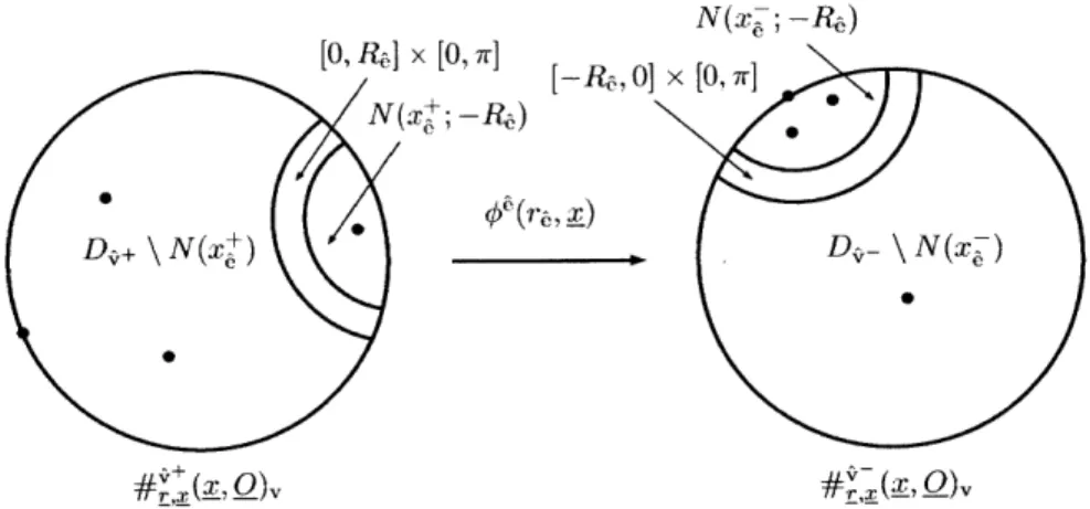
to (j4, ig) (in the sense that (xv, uj ) E U,,:: ig) as in Definition 4.1), with coincidence condition (2.9) satisfied. Then we define the gluing map as follows

[#: (-c )nd x UE(f) -+ X (1.1)

(r, (T,, x, u)) e[ri,#() ,() ru]

For each nodal edge =

(-,

+) End with gluing parameter rc > 0, we identify

9~

and

9+

to a single vertex in the glued tree #,(t). Take an re-dependent strip near xg-, in the disk De- and an re-dependent strip near xc,+-Z in the disk D,+, glue the strips together to get a glued disk, and then discard x ,- ,6 and x,+,6 in the glued boundary marked points

#r (x); moreover, we interpolate the nodal map (u ,+,ug-) on the glued strip to define a

map on the glued disk (see (4.14)). On the other hand, for each edge

6

= (-+) C t with r& < 0, we displace the w- part of the nodal map (u4+,

u.-)

along the Morse flow so that uj+ and up- become separated (see (4.15)). This gives rise to the tuple of maps

#x,,(u), and the new Morse flow between the pair is the displaced Morse trajectory #r(Y)

(see (4.8)).

Now imagine the gluing parameter r6 decreases from positive to negative, this curve in X does not stop at the bubbling at r6 = 0 when a map becomes nodal, but it continues displacing along the Morse flow when r becomes negative. In this way, disk bubbling is an

interior point in X; the boundary and corners structure of

I

comes from that of the Morse trajectory space. Later on we shall use this fact to prove that the AC, algebra we construct indeed satisfies the A,_ equation.

Let K. be the equivalence class [f]. We denote the image of [#] in (1.1) by it, (K;

f).

This collection of neighborhoods arsing from gluing defines a Hausdorff topology (Theorem 4.6).

(15)

Theorem 1.3. The collection {,(n;

#)

Ic E it} forms a basis in X and defines a Hausdorff topology.

We now briefly describe the M-polyfold with boundary and corners atlas (see [7]) for X

the quotient space of disk trees. We shall construct a chart around a disk tree r. by using

a variation of the gluing map [#] : (-e, c),nd x U -(f) iT in (1.1). Note that the gluing

map [#] itself is not a chart. It is not injective due to (1) the conformal disk automorphism action on each disk, and (2) the interpolation on the glued strip used in the gluing. We deal with problem (1) by restricting the domain to a "slice" of the neighborhood U(f), and handle problem (2) by further restricting to a subset of maps called the "splicing core". Hofer, Wysocki, and Zehnder built M-polyfold theory with problem (2) in mind, adopting splicing cores as local models of the M-polyfold (see [71). This collection of charts forms an atlas (Theorem 6.12).

Theorem 1.4. The quotient space of disk trees X has an M-polyfold with boundary and corners atlas.

With some additional minor topological properties of X, Theorem 1.3 and Theorem 1.4 essentially constitutes Theorem 1.1.

In order to prove the above results on the topology and the atlas of the quotient space of disk trees, we study the Deligne-Mumford space 9J1, a finite dimensional analog of

i. We refer the readers to [19], [181, [16], [14], and [10] for studies of other cases of the Deligne-Mumford space.

The Deligne-Mumford space with k incoming critical vertices 09JI(k) consists of equivalence classes of the form [T, f, x, 0]. Here T is an ordered tree with a partition into

main vertices and critical vertices V = Vm U VC, with critical vertices consisting of k leaves and the root rt(T). The tuple f consists of edge lengths f, E [0, 1] for each edge e C E.

The tuple (x, 0) consists of boundary marked points and interior marked points (4,! OV)

for each main vertex v E V, where each 0, is unordered. Furthermore, the tree of marked points and edge lengths satisfies the stability condition (i.e., each main vertex v with no interior marked points O, = 0 is associated with at least three edges as in equation (5.1)).

(16)

Lastly, the aforementioned equivalence relation is given as follows. We say (T,

e,

I,

o)

is

equivalent to (T', l', x', o') if there is an ordered tree isomorphism

(

T -+ T' and a tuple of conformal disk automorphisms 0' (OV)IVem such that

*

(

relabels the edge lengths f =,, and

* '

push forward the marked points to the marked points relabeled by

(,

(VI(11V), ( ))=

(I,,, O

'),).

In this case, we write ((,0)(T,-y, , u) = (T', , I').

We use gluing to construct a topology and an atlas on the Deligne-Mumford space '91 in an analogous way to X. Let

ft:

(,

L,

,) be a representative. Denote by

End

the set of nodal edges, whose edge lengths & are 0; we introduce a gluing parameter r6 E (-E, -) to each nodal edge. We define the

E-neighborhood

U,(f) and the gluing map in a similar way as in the quotient space of disk trees

[# : ) (-t,) x )9 2(1.2)

(r (,

, X, 0))

[#,. J), #' (f), #' (j), #_rX (Q).

We displace the edge lengths #r(_) in an analogous way as we displace Morse trajectories

#,r(),

keep the glued boundary marked points #,(,) as before, and define the glued interior marked points

#,,,(0)

to be the union of interior marked points on the glued disk.

The Deligne-Mumford space has the structure of a manifold with boundary and corners (Theorem 5.18). Much like the boundary of quotient space of disk trees is given by elements with broken Morse flow lines, the boundary of the Deligne-Mumford space is given by elements with unit edge lengths.

Theorem 1.5. The Deligne-M'umford space

91

is a manifold with boundary and corners.

While the above result does not directly prove Theorem 1.3 and 1.4, the tools we develop along the way are instrumental to proving the M-polyfold structure of X. Here we roughly

(17)

sketch this idea. For a disk representative (T, _y, x, u), we can construct a set of codimension 2 sub-manifolds of M that are transversal to the disk maps u. We call them transver-sal constraints. We then locally define a stabilization map which takes (Tyx,

u)

to (T,

f,

x, Q), where each 4 is the renormalized length of the Morse trajectories - (see (2.2)), and each 0; is the pre-image of the transversal constraints under the map ujv. The stabiliza-tion (T,

f,

x,

Q)

is a representative of an element in the Deligne-Mumford space. Suppose we have equivalence of gluing

((

4)(#(r,

(, x,_u))) = #(n', (T', J ', X', ')),

where

#

is the gluing in (1.1) before taking the equivalence class. Then the same ((,

4')

gives equivalence to their stabilizations

((, 'V)(#(n,

(T,4, x,O))) =

#(', ('', x',O')).

Thus understanding how

((,

4)

depends on the gluing parameters r and the stabilization (T, t, x, 0) help us understand the gluing map (11.19), which help us prove the topology and the atlas of X. We refer the readers to Proposition 5.23 and 8.11 for further details.

We now work towards constructing an A.. algebra. Firstly, let 7r

9

- X be the bundle of complex anti-linear sections, where T consists of equivalence classes of the form [T, y, x, _t,

A].

The fiber consists of tuples

A

= (Av)vEvm such that for each main vertex v C V"' and point z C D,

Av (z) : (Tz D, i) --- (Tuv_,)M, J(uv(z)))

is a complex anti-linear map. Moreover, we require each Av to have H26 regularity. We define the Cauchy-Riemann section d: X -÷

29

by

1

&j(u') = -(&su + J(Uy) atuv).

2

(18)

show that the Oj section is sc-Fredholm (Theorem 9.10).

Theorem 1.6. The bundle of complex anti-linear sections 7U : -* X is an M-polyfold

strong bundle, and the section Oj : X -+

23

is sc-smooth and sc-Fredholm.

We are now in the right position to construct an A,, algebra from the quotient space of disk trees. For each disk tree z = [T,,x,u] E ([Pk ( .. 0 p1, q; t, v), we call [Pk 0

--

pi,

_{q; p] the type of z. Suppose two disk trees zv} _{C X([pk}₀_- _{0, p, q; t], v) and}

zw E X([rl -- -0 ri, s; 6], o) are such that q = ri. Then we can concatenate the Morse

trajectory in z' which flows into q with the Morse trajectory in z' which flows out of ri and obtain a concatenated disk tree. In general, for a tree of disk trees such that all

edges

e

= (v, w) satisfy the above coincidence condition at critical points, then we define their concatenation similarly as before (see Definition 11.9 for details). We denote the concatenation operation by o, and note that a concatenated disk tree lies on the boundary of X because it has at least one broken Morse flow line.

One can find a sc+ perturbation (see Section 1.4 of [7]) of Oj which is compatible with the concatenation o, and the perturbed solution set has a compact manifold structure (Theorem 11.15 and Theorem 10.9).

Theorem 1.7. There exists a o-compatible sc+ section s : X -+ 2) such that for all types

Z and v > 0, the solution set of the perturbed section (Oj + s)>1(0) n X(Z, v) is a compact manifold with boundary and corners.

In order to define the desired A,,, we shall focus on those disk trees with Fredholm index 0. By an index calculation, all disk trees z of a fixed type Z = [pk G .. -0

pi,

q; p] have the same 6j Fredholm index

k

indo,(z) =- indj,(Z) = 1pil - JqJ + p - (k - 1)(n - 1) - 1. (13)

We construct the disk tree A,, algebra over Z2 as follows, using the Novikov ring

(19)

Here e is the quantum variable. In the sum, there are finitely many non-zero ci with vi < N for any N. Let C be the complex generated by Morse critical points

C = E A(p).

pEcrit(L)

The total complex C = D &k C has an obvious bilinear form

ApP, A' P) ApA'p E A,

where we sum over pure tensors P = 0 -- 0 P1 with pi C crit(L). For each k >

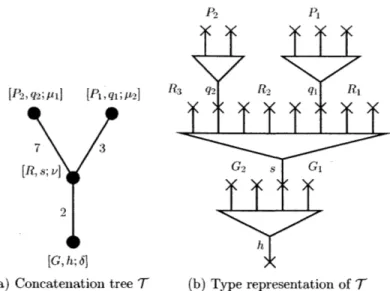
0, define the k-th multiplication mk : &k C .. C as follows. Given a pure tensor of critical points R = rk 0 - - 0 r, and a critical point s, we denote by

p*

the integer such that indoj([R,s; p*]) = 0, which we calculate from (1.3). We denote the perturbed section f := Oj + s, with perturbation given by Theorem 1.7. Hence the solution set

f 1(0) n X([R, s; p*], v) is a compact 0-dimensional manifold. We define the coefficient

(Mk(R), s) by taking the Z2 count of the above solution set

(m(R), s) := nz2(f (0) n 3([R, s; p*I, v)) eV. (1.4)

v>O

Naturally, we have mk(R) = Esecrit(L)( k(R), s)s. We then extend the multiplications to m : C -+ _{C in the standard way ([13]) as follows. Given a pure tensor P = A} ₀_O _pi,

we denote its length by JPJ = k. We define

Wi(P) = P2 0 m 1 (P') &P1, (IP', jP~I potentially 0) (1.5)

P=P20P'OP1

and then extend A-linearly to combinations of pure tensors. The extension ih satisfies the

A,, algebra equation

ih o i-n = 0 (1.6)

since the boundary of a 1-dimensional solution set is precisely given by disk trees with once broken Morse flow lines, which are the concatenations of two index 0 solutions. Thus (C, Fh)

(20)

is a curved A,, algebra (curved means i does not necessarily vanish).

Thus we finish constructing an Ao, algebra (C, ih) by choosing any compatible

almost-complex structure J and some sc+ perturbation s. In order for (C,ih) to be a syiplectic

invariant, we would like to show that the A, algebra is independent of the choice of pairs

(J, s). More precisely, given two such pairs (J-1, s_1) and (J1, s1) and let (C, i-1) and

(C, Th1) be their respective A, algebra, we need to construct an A, isomorphism between

(CJi_1) and (C,iri1).

To prove the above result, we first find a smooth 1-parameter family of almost-complex structures (Jt)tE[-1,I between J_1 and J₁. We can do this since the space of almost-complex

structures compatible with w is connected. The difficult part is finding a 1-parameter family of o-compatible perturbations (st)t,[-,1 so that the family of sections

F :[1, 1 ] x X -+Q), (t, x) (Oj, + st) (x)

achieves a certain special transversality condition. The transversality problem is compli-cated by the presence of index -1 solutions at certain irregular t E (-1, 1): index -1 solutions

can potentially concatenate with itself for arbitrarily many times and the results are still index -1 solutions. In this thesis, we deal with a special case when F is assumed to be o-transverse, which limits the number of ways an index -1 can concatenate with itself

(Theorem 1.8).

Theorem 1.8. Suppose there exists a 1-parameter family of o-compatible sc+ perturba-tions so that the family F(t, x) (6j, + st,)(x) is o-transverse, then there exists an A,

(21)

Chapter 2 Quotient Space of Disk Trees

Let (M, w) be a symplectic manifold of dimension 2n with wt,,(A) = 0, and L a Lagrangian submanifold of M. In addition, we choose a compatible almost complex structure J on M, and a Morse-Smale pair (f, g) on the Lagrangian L.

In this section, we define the quotient space of disk trees

,T([pk & .. - pi, q; p], v).

We first go over the standard notions of an ordered tree and a Morse trajectory space.

2.1 Ordered Tree

A tree T is a connected graph with no cycle. Let us denote by V the set of vertices, and by E the set of edges. A rooted tree is a tree with a designated root vertex rt(T) E V. Let the edges be oriented towards the root. The orientation on the edges induces a partial ordering on V, known as the tree order, where the root rt(T) is the maximal element. This allows us to think of E as a subset of (V x V) \ A. More precisely, for two adjacent vertices v and w with v < w, we denote by (v, w) the edge going from v to w; we call v a child of w, and w a parent of v.

(22)

edges and outgoing edges of v are given by

E(v) :={(w,v) E E}, Eo"t(v):= {(v,w) E E}, (2.1)

respectively. The set of all edges of v is given by E(v) := Ein(v) U Eout(v). A vertex

v

is called a leaf if Ei"(v) =

0.

We note that Eo"t(v) is empty if v is the root, and has a single element otherwise. We define the valency of a vertex v to be the cardinality of E(v), denoted as lvi.

If T is a rooted tree and each set Ei"l(v) has an order, then T is called an ordered tree. Then we can order the set E(v) as

E(v) ={C(v) e Vj(v)}. (2.2)

For v

f

rt(T), we choose

e

0_{(v) to be the outgoing edge of v. This order induces an ordering}

of all children {w C V I (w, v) E Ei"(v)}. Combining this order with the tree order induced by the orientation of the edges, we get a lexicographical ordering on the set of all vertices.

(

: T -+ T' is a an ordered tree isomorphism if it is a bijection between V and V' which preserves the lexicographical ordering, and induces a bijection between E and E'.

It is straightforward to verify the following uniqueness result for ordered tree isomor-phism.

Proposition 2.1. If

(

T -- T' and

(

T -+ T' are both ordered tree isomorphisms, then

2.2 Morse Trajectory Space

Another essential element of the quotient space of disk trees is the compactified Morse moduli spaces. Here we give a short introduction. For more details, we refer the readers to [20]. Let (f, g) be a Morse-Smale pair on Lagrangian L. For p C crit(L), we denote by

IpI

the Morse index of p.

(23)

For p

#

p+ E crit(L), we define the space of Morse flow lines from p- to p+ modulo

the R-shift action as

M(p- p+) {y :R -+ L = -Vf(7), lim -y(s) = pI}/R.

S- + 00

For p- = p+, we set M(p-,p+)

0.

We recall from Morse theory that M(p, p+)

0

if

Ip-I

<

Ip+

1. Now we define the space of half-infinite Morse flow lines.

M(p-, L) := {y: (-o, 0] - L -Vf (y), lim -(s) = p-}

$-+-00

M (L, p+) {y : [0, c) - L = -Vf (y), lim y(s) = p+.

Lastly, the space of finite Morse flow lines is

M(L, L) := {y : [0, a] -+ L I a > 0,,y -Vf(y)}.

The above spaces of Morse flow lines admit a compactification by adding the "broken Morse flow lines". To be precise, let U be either L or a single critical point, then we define the

Morse trajectory space as

M (U-, U+)

U

M(U-pI) x M(p1,p2) x x M(pk,U+).

kENo, P

I>--->|Pkl

An element -y = (70, -Y, .... , Yk) is called a generalized trajectory, which represents a

broken flow line when k > 1. The Morse trajectory space A4(U-, U+) can be given the smooth structure of a compact smooth manifold with boundary and corners.

To specify the topology of

M(U-,

U+), we define the following length.

Definition 2.2. We define the renormalized length

f(-y)

of a generalized trajectory -y by,

if : [0, a] -h+ L,unr= okO

(24)

Note that the renormalized length can distinguish trajectories in A4 (L, L) with image being a single critical point p and broken trajectories in A (L, p) x Al (p, L) with the same image. We now give M(U-, U+) the topology induced by the following metric.

d-F-(,, i) := dHausdorff (Im-Y, im?7) + [ (Y) - FW 1 (2.3)

where im7 = imyoU- --Uimyk. We recall the definition of Hausdorff distance in the appendix (Definition 13.5).

For a broken flow line = (O, 1,... ,

I')

and small

e

> 0, there is a diffeomorphisin (onto its image) called Morse gluing map (see [20])

B,( O) x [0,e) x B,(, 1) x -- - x [0, e) x B,('k) -+ M (2.4)

(-o, ri,yi1, .... , re7'k 7 ) -" r(_7),

where r = (ri,... , rk) _{are the gluing parameters. The trivially glued Morse trajectory}

_yo(Y)

is equal to y, and if all ri are positive, the glued Morse trajectory

(_)

is unbroken. More-over, for trajectories y = (y1,7 ', 2) and parameters r = (r, r' r2_),

we have associativity

This map later plays a crucial role in our Ao algebra.

Definition 2.3. We define the evaluation map on these Morse trajectory spaces as follows.

" Define ev x ev+ : M (p-, p+) {p-I x {p+} by ev-(y) = p-, and ev+(Y) P+

" Define ev- x ev+ M(L, p+) L x {p+} by ev-(yo,. .., _Y) = -yo(0), and ev+(y) p+.

" Define ev~ x ev+ :M(p-, L) -+ {p-} x L by ev-(-) = p~, and ev+(-yo,. . . , Yk) = Yk(0).

" Define ev- x ev+ :AM(L, L) -+ L x L by ev-(yo, ... yk) = 0(0), and ev+(YO... k) Yk (0) for k > 1 or ev+(-7 : [0, a} -+ L) = yo(a).

(25)

2.3 The Quotient Space of Disk Trees

We now define the quotient space of disk trees as a set. Let Pk, .. . , pi, q be critical points, p an integer, and v a non-negative real number. The quotient space of disk trees with incoming critical points pk,... ,pi, outgoing critical point q, and p E Z, v > 0 is

denoted by

:E([pk 0 ... - pi, q; t], v) := {(T , ,u)

1(1)

- (4) satisfied} /~igh. (2.5)

We define conditions (1) - (4) and the equivalence relation ~bihol as follows. (1) T is an ordered tree with the following requirements.

* The root rt(T) has a single edge, i.e., Irt(T) = 1.

* The tree T is equipped with a choice of a partition Vm U V' = V, into the set of main vertices V"', and the set of critical vertices Vc, such that rt(T) E VC, and Vc

\

{rt(T)} consists of exactly k leaves (same k as in (2.5)).

(2) ), ()eEE is a tuple of generalized Morse trajectories with the following requirements.

For each critical vertex v E Vc, we assign pv C critf in the following way. The set of critical leaves VC \ {rt(T)} has exactly k elements, with an order induced from the lexicographical order of T. Hence VC \ {rt(T)} = {wk .. ., wi}. We define

Pw := Pi, Prt(T) =

where pi's and q are the Morse critical points given in (2.5). For an edge e = (v~, v+),

the generalized Morse trajectories - are required to have ends on these critical points as

(26)

MA(py, +, M(pv-, L), Le, A4(L, Lv), for v-, v+ C VC, for v- C VC, v+ E V"T for v- E" m"v+ C VC, for v-, v+ E Vi.

(3) (,

u)

= (vuv)vcnvm is a tuple of boundary marked points and disk maps with the

following requirements.

* For each main vertex v c V" and each edge e C E(v), we associate a boundary

marked point ve C OD. Furthermore, these marked points xv,,e are distinct, with

Xv,eO(v) ... v,e-1(v) positioned counter-clockwise on OD (see the labeling in (2.2)). We denote this ordered set of boundary marked points by

1V = {xv,e C OD Ic c E(v)}.

* For each main vertex v C V"', the disk map uv has regularity H3,o ((D, xv), M).

(Roughly speaking, uv has three weak derivatives and exponential decay near the marked points r. See Section 3.3 for the precise definition.) Moreover, v satisfies the Lagrangian boundary condition,

uv(OD) C L.

Then it follows that uv represents a relative homology class in H2(M, L). We define w(uv) to be the coupling

(2.6)

and we require w(uv) > 0.

It is sometimes more convenient to use an alternative way to index boundary marked points follows.

(27)

and disk maps by edges e = (v-, v+):

Xe :=Xv ,e, Ue :=uv . (2.7)

(4) The tuple (T, y, 1, i) satisfies the following additional requirements.

" A main vertex v E V" is a ghost vertex if w(uv) = 0. We impose the stability condition, that is,

for a ghost vertex v, we have IvI > 3. (2.8)

" For each edge e = (v-, v+) E E, we impose the coincidence condition defined by the evaluation map (Definition 2.3),

ue (x4) = evi ) if vi

E

V'. (2.9)

" Denote the Maslov index of uv with respect to L by p(uv) E Z. (See Appendix C.3 of [15] for a complete exposition of boundary Maslov index.) For p E Z and

v

> 0 in (2.5), we impose the topology condition

P(uV) = A, w(UV) = v. (2.10)

vEVr vEV

Lastly, we define the equivalence relation

~bihol-Definition 2.4. We say (T, -y, I, u) is equivalent to (T', -y', x', u') via a biholomorphism if there exists a tree isomorphism

(

: T -> T' and a tuple of disk automorphisms

@

(''v)vEVI (see Section 13.1) such that

*y = yfor every

e

E E and

c' =

((e),

* 'v(XV,e) =, for every v E Vm,

e

E E(v) and v' = (v), e' =(e),

(28)

In short, we write ((, ')(T, , x, u) = (T', , ', u'). Moreover, we write an equivalence class

under the relation ~bihol as

[T,-, x, u].

Finally, we define the quotient space of disk trees by taking the union

X := J X([Pk 0 ... 0 pi, q; pl, v) (2.11)

over all k E No, all critical points pi and q, and all p E Z and V > 0.

The following result shows that each element (T, -y, x, u) has trivial isotropy group.

Proposition 2.5. Suppose there are two biholomorphisms (',$) and

(,

y)

which satisfy

( _)( , ((,T)(T,, x, u).

Then we have

(C,

) ={, b).

We shall prove this result later by using a transversal constraint to pass onto the Deligne-Mumford space. Most importantly, we shall give X an M-polyfold structure.

(29)

Chapter 3 Polyfold Smoothness and H

3 ₁

6 ₀

Maps

As we shall see later, an M-polyfold is locally modeled on certain subsets of sc-Banach spaces, a type of Banach space with an infinite nested sequence of Banach spaces with certain properties. In [7], Hofer, Wysocki, and Zehnder define a smooth structure on sc-Banach spaces. In this section, we define the topology of the space of boundary marked points and disk maps using sc-Banach spaces.

3.1 Sc-Banach Spaces

We first define the notion of an sc-Banach space, which provides a foundation for the polyfold smooth structure. We refer the readers to [7] for an in-depth introduction.

Definition 3.1. An sc-structure on a Banach space E consists of a nested sequence of Banach spaces (Em,)mnENo with EO = E, and each Em+ is a linear subspace of Em but with possibly different norms. Moreover, this sequence of Banach spaces must satisfy the following two conditions.

1. The inclusion maps Em+i + Em are compact operators.

(30)

2. The space E Fi

:=

rn E,,. is dense in every E,,.

A Banach space E equipped with an sc-structure is called an sc-Banach space.

Here we present two examples of sc-Banach spaces which are crucial to the quotient space of disk maps: one for the regularity of a disk map away from the marked points, and another for the regularity near the marked points under certain strip coordinates.

Example 3.2. Let V C Rk be a bounded domain with Lipshitz boundary in the Euclidean space, and H'(V, C") the Sobolev-m function space. The space E = H3(V, C") is a sc-Banach space with sc-structure

E

= H3+"n(V, C"). Indeed, it follows from the compact

embedding theorem that the inclusion Em+1 -+ E,,, is compact. Lastly, we have E, C (V, C") and the space of smooth functions is dense in every E,.

The reason for choosing H3 space as the

0-level sc-structure is that the Sobolev

embed-ding theorem guarantees H3 -+ C', and later on we shall use the first derivative of disk maps in our construction.

The following example describes the sc-structure of maps on the infinite strip that take value in C' with boundary condition on

R".

This is a local version of the Lagrangian boundary condition.

Example 3.3. We define the weighted Sobolev space

H'4(R x [0, 7r], C"; R')

as follows. Let

f

be a function whose weak derivative O'f is locally represented by an L2 function, where the multi-index a is of order

lal

less than m. Then the norm

II

m is

defined by

|f

IIams

:= < I r

f

(s, t)I2e2IjsIdsdt. (3.1)

The space H',6 (R x [0, 7r], C";

Rn)

consists of all functions

f

whose norm 11f 11|n,s is finite with each f(s, 0), f(s,

7r)

E

Rn.

We refer to 6 as the weight.

Let E be H3,6o (R x [0,

7r],

C"; R") with 6o > 0. Given a strictly increasing sequence

(31)

[0, 7], C'; R') is an sc-Banach structure. Indeed, one can use the compact embedding for bounded domains and the increasing weights to show that the embedding E7 +, -- Em is

compact. Lastly, the E,, space is the set of smooth functions with the proper decay; it is dense in every Em because the space of compactly support smooth functions is dense.

As a variation of the weighted Sobolev space, we define the weighted Sobolev space with limits

Hg(R x [0, 7r], C'; R')

to consist of functions

f

with limits c C R" such that

f

- c lies in Hl 6 (R x [0, 7], C'; Rn).

We define the norm

11f 112, :c12

+f

- C|,6

Let E be H "(R x [0,w],C"; R') with 6o > 0. With strictly increasing weights 6o <

6_{, <}

... , the sequence Er = H m (JR x [0, 7], C; Rn) is an sc-Banach structure. We now introduce the concepts of sc-operator and partial quadrant.

Definition 3.4. Let E and F be sc-Banach spaces. A linear map T : E -* F is an

sc-operator if we have T(Em) C Fm for all m c No and the restrictions T : Em -+ Fm

are continuous. An sc-operator is an sc-isomorphism if its inverse is also an sc-operator. Lastly, a subset C C E is called a partial quadrant if after applying an sc-isomorphism

it is of the form [0, OO)k x W for some sc-Banach space W.

Going beyond linear maps, we now discuss the notions of continuity and differentiability in Banach spaces. Let U and V be open subsets of partial quadrants C and D in sc-Banach space E and F, respectively. We denote their m-level by Um, := U

n

Em, and V,, :V n F..

Definition 3.5. A map

f

: U -+ V is sco if we have f(U,) C Vm for all m E No and the restrictions

f

: U -+ V, are continuous.

We denote by Uk the k-level set Uk with sc-structure Uk := Uk+mr. Define the tangent space TU by

(32)

Definition 3.6. An sco map

f

U - V is said to be scl if for every x E U there exists a

bounded linear operator Df(x) Eo -+ Fo such that the following holds.

1. For h E E1 with x

+

h E C, we have the limit

lim If (x + h) - f(x) - Df(x)hlo = 0.

jt,,j-+o Ih|1

2. The tangent map Tf : TU -+ TV defined by

(x, h) '-* (f(x), Df(x)h)

is sc0.

We say

f

is sc2 if the tangent map Tf is sc1. Inductively, this defines the notion of sck.

We say

f

is sc-smooth (or sc*) if

f

is sck for all k.

One key distinction between sc-differentiability and classical differentiability is that the continuity of (x, h) -* Df(x)h as in scl is weaker than the continuity of x - Df(x) in

operator norm as in Cl; Proposition 4.2 of [7} shows that the reparametrization action on a cylinder is sc-smooth but not classically smooth. We refer the readers to Proposition

1.9 and 1.10 of [7] for a thorough study of the relationship between the sc and classical

differentiability. Furthermore, Theorem 1.11 of [7] shows that this generalized smooth structure has a chain rule. Lastly, an M-polyfold is locally modeled on certain subsets of se-Banach spaces called sc-retracts (Section 6.1). These subsets are the images of certain sc-smooth retractions, and they are not generally open in their ambient sc-Banach spaces.

3.2 Boundary Marked Points and Strip Coordinates

As we shall see in the Section 4, we define the topology of the quotient space of disk trees - using gluing. The construction of a glued disk map involves viewing neighborhoods of marked points in the disk as half infinite strips, truncating them to certain lengths, gluing

(33)

them pair-wise, and interpolating the maps on these glued strips. In this section, we define the space of boundary marked points and the strip coordinates near them.

We denote the space of boundary marked points by

MVP(aD) :=x C aD I -= (XO, . .. ,Xk) for k > , . (3.2) distinct and ordered counter-clockwise

The underline in MP(aD) emphasizes that the boundary marked points are ordered. This space has a metric

d(x, x')

{

maxi dOD(Xi, x ) if n(x) =

100 if n(x)

#n(),

where n(x) denotes the cardinality of

x.

We denote the c-neighborhood of 1 in MP(aD) by

Upe~).

We now introduce the notion of strip coordinates near a boundary marked point. Let us denote the half-infinite intervals by

R+ := [0, oo), R- := (-oo, 0].

Definition 3.7. Let x be a boundary marked point. A biholomorphism into a closed neighborhood N(x) C D of x

h+ R+ x [0,

ir]

- N(x) \ {x}

(or h- R- x [0, 7r] - N(x) \ {x})

is called positive (or negative) strip coordinates near x if it is of the form

h* fOP,

(34)

p: R x -+ {0 < zI < 1, Iiz >

01

are given by

P+(Z) := -e-Z -)

* f

is a Mbbius transformation that maps the extended upper half plane {Imz >

0}

U {oo} to the disk D with f(0) = x.

The closed neighborhood N(x) is called a strip neighborhood of x. We also consider a family of such strip coordinates.

Definition 3.8. Let - be a boundary marked point. Suppose there is a smooth family of M6bius transformations

f..

for x C L4(Z) such that

"

each

f.

maps the extended upper half plane {Imz > 0} U {oo} to the disk D, and * fx(0) = x and fx(oc) is independent of x (i.e., f,(oc) =fj~o)).

Then we call h (x, . _{op+ a family of strip coordinates near -. For each x}C t5-(&), we have strip neighborhood N(x).

Note that the limit of a family of strip coordinates is the same as the boundary point x

lin h+(x, z) = x.

z-* ,:!,

For

R

> 0, we denote the shrunk strip neighborhood by

N(x; -R) := {x} U h+(x, [R, oo) x [0, 7r]),

{x} U h-(x, (-oo, -R] x [0, r).

Note that N(x; 0) = N(x) and N(x; -R) shrinks to the marked point {x} as R -+ oc. Remark 3.9. If ht(x, -) is a family of strip coordinates near a% and '< is a disk automor-phism, then k+(x,-) :=

4' o

h'( r(x), -) is a family of strip coordinates near

(35)

Remark 3.10. Recall from (2.2), for a main vertex v E V"i,

co(v)

is the outgoing edge,

and e1(v), ..., _{e' (v) are incoming edges. For boundary marked points x}= (xo,. . ., Xk), we

assign negative strip coordinates

h-

near the outgoing marked point xO, and for each i > 1 we assign positive strip coordinates h+ near the incoming marked point xi. Thus we have a tuple of strip coordinates h = (h-, h,...,

h)

near x.

In our topology of the quotient space of disk trees, we allow the boundary marked points to vary while fix the complex structure on D to be the standard complex structure. However, in the polyfold theory for Gromov-Witten in [8], the marked points are fixed, whereas the domain complex structure can vary. These two approaches are equivalent. In the following lemma, we explicitly constructs a family of diffeomorphisms v. : D -+ D defined for each

x E U,(). It maps the fixed marked points _s on the disk (D, v* i) with varying complex

structure to the varying marked points

x

on the standard disk (D, i). We shall use this family of diffeomorphisms in the construction for the topology of the space of boundary marked points and H 60 disk maps in Section 3.3.

Fix boundary marked points , = (-'6,. . ., 4), and let B(.s) C D be mutually disjoint open subsets of D containing

z.j

Let

h = (h-(xo, -), h+(xi, ), ... ,h(,

be a tuple of families of strip coordinates near

1.

Choose e > 0 small enough so that for all

x E U(.), each strip neighborhood N(xi) is contained in B(,i).

Lemma 3.11. There exists a smooth family of diffeomorphisms us : D -+ D defined for

each x C Ue(.) with the following properties.

"

Vu. (z) = z for z LJ- B )

" If x is such that xi =

i

for some i, then vx(z) = z for z G B(., ).

" Vu(z) = fXi o

f1'(z)

for z

c

N(.i .), where fxi is the Mibius transformation in

(36)

In particular, twe have vj. Id. Moreover, v xi, and v,, maps the strip neighborhood.(ri)

N( j) biholomorphically to N(xi). It also transports strip coordinates in the sense that vxo h' ,-) = h:(xi,

We can construct such a family of diffcomorphisms via integrating vector fields. In the fixed marked points and varying complex structure model, the last property translates to saying the complex structure (D, v4 i) is the standard i near the fixed marked points , . As we shall see, the last property is crucial in the topology of the space of boundary marked points and HJo disk maps.

3.3 W the Space of Boundary Marked Points and H

3

_{.o Maps}

In the description of the quotient space of disk trees, the space of boundary marked points and disk maps plays an important role. In this section, we define a topology on this space.

Recall that L is the given Lagrangian submanifold of the symplectic manifold M.

Fix m > 3 and weight 6 E (0,1). Let x (Xo,..., Xk) E MP(&D) be boundary marked

points.

Definition 3.12. Choose open neighborhoods U of u(xi) in M, along with C charts Ui

: Ui - B1(0) C C" with yai(u(xi)) = 0 and p1(L n U) = R' n B1(0). Also choose strip

coordinates h such that the strip neighborhoods N(xi) satisfies u(N(xi))

c

U. We define

Map'rr((D, x), Al; L) the space of H"'5 maps with marked points x and boundary condition L to be the set of u : D -+ M with the following properties.

" The restriction uID\U N(i;--1) belongs to H'(D\Ui N(xi; -1)), where each N(xi; -1)

is the shrunk strip neighborhood (see (3.3)).

" On the strip neighborhood N(xi), the local expression in strip coordinates pj o u o h belongs to H"6 (R1 x [0, ], C"; Rn) (see Example 3.3).

(37)

One can show that the above space is well-defined, i.e., independent of choices of charts p and strip coordinates

h.

It is independent of choices of charts by Proposition 13.18. Moreover, suppose we have two strip coordinates hP and h,' . By Lemma 13.17, the map

(h')-1

o h'

satisfies the conditions in Proposition 13.16. Then it follows from Proposition 13.16 that u o h' belongs to H"', if and only if u o h' = (u o h ) o ((ha) o h,' ) belongs

to H"mk. Thus the above space is independent of choices of strip coordinates.

Remark 3.13. We choose Map36

o

to be our base regularity. To give the readers an idea of the smoothness of maps u c Map36o, the Sobolev embedding theorem guarantees that u is C' away from the marked points x. However, one can show that the weight 60 < 1 is not large enough to grant C' regularity at x, but it does guarantee Co. In our future

construction, we shall take advantage of the first derivative in the interior of the disk.

Remark 3.14. Here we highlight a small difference in convention with the work of Hofer, Wysocki, and Zehnder. In our Definition 3.7, coordinates pt are defined on half-infinite strips R x [0, 7r] by

p+(s

+

it) =-e-(s+it), p-(s + it) = es+it.

In the setup under Theorem 2.1 of [8] however, coordinates p are defined on half-infinite cylinders

R

x S' with

S'

:= [0, 1]/o-,1 and they are given by

p+(s + it)

= e-2,(s+it), p+(s

+ it)

= e27(s+t).

The factor of 27r scales the weight 6 accordingly. In particular, the sc-smoothness result in Theorem 2.7 of [7] requires the weight 6 < 27r. Here we require 6 < 1.

As we have seen in Section 2.3, the space of boundary marked points and H3,60 disk maps plays an essential role in the quotient space of disk trees. We now define this space and give it a topology later on.

Definition 3.15. We define W the space of boundary marked points and H3,6o maps

(38)

by

W := {(x, u) I v MP(OD), u E Map3,6((D,x),M; L)}.

In order to define a topology on I, we first consider the space of sections at a given disk map.

Fix m > 3 and weight

6

E (0, 1), and fix boundary marked points x = (x₀,...,

xk)

E

AIP(OD) and disk map u E Map'rn,6((D, x), M; L). Let u*TM -+ D be the pullback bundle. We now define the Banach space of H',6 sections of the pullback bundle.

Definition 3.16. Choose C' charts _p and strip coordinates It as in Definition 3.12. We define Sec'fl((Dx), u*TM; TL) the Banach space of H'"6 sections of u*TM with marked points x and boundary condition TL to be the set of : D -+

uTM*

with the following properties.

" The restriction c ID\Lji N(xi;-1) belongs to H"(D\_J N(xi; -1)), where each N(xi; -1) is the shrunk strip neighborhood.

" On the strip neighborhood N(xi), the local expression in strip coordinates

f(z) :=Diuh()((?z)(3.4)

on RL x [0, 7r] _{belongs to the weighted Sobolev space with limits}

(

_E_H;(Rn _x [0, 7r], C; R") (see Example 3.3).

" (z) ETutz)L for z C OD.

Choose a Riemannian metric g on M, we now define a norm

k

II(|I2 := l(D\Lj N(xi;-1) Hm HmI , (3.5)

i=O

where the norm

|ID\Uj

N(xi;-1) Hm is defined using the metric g and its covariant derivative

in the standard way.

Similar to Definition 3.12, one can show that the above space is well-defined, i.e., inde-pendent of choices of charts o and strip coordinates h. Moreover, different choices of metric

(39)

g, charts, and strip coordinates give equivalent norms (3.5).

Remark 3.17. Suppose disk map it lies in Map3+ ." ((D,

x),

M; L) for all

m

> 0, with'

strictly increasing sequence of weights 6o < 61 < ... < 1. The nested sequence

Em, := Sec3+nt'n ((D, x), u*TM; TL)

defines an sc-structure on Sec33

o

((D, x), u*TM; TL). We shall use this sc-Banach space to construct an M-polyfold atlas in Section 6. Note that such sc-structure is not defined for general disk map u E Map3,60 because local expression in (3.4) involves u as well.

We now proceed to define a topology on W by defining a neighborhood basis around each (i, f) E W. Firstly, by Lemma 4.3.3 of [151, there is a metric on M such that L is totally geodesic.

Lemma 3.18. There exists a Riemannian metric g on M such that the Lagrangian L

becomes totally geodesic, i.e., every geodesic of the submanifold L is a geodesic of the ambient manifold M.

Choose such a metric g. For a section

c

Sec3 o((D,4), fi*TM; TL), we use the expo-nential map of (M, g) to define a disk map expa o (: D - Al

expf o (z) = exp,&(z)( (z)). (3.6)

The map expa o belongs to Map3,o ((D,; ), Al; L). Indeed, using standard analysis of Sobolev spaces and the smoothness of the exponential map, one can verify the first two properties of Definition 3.12. Moreover, for a boundary point z

c

OD we have expf o (z) E

L, since (z) E Ta(z)L and L is totally geodesic.

Using the family of marked points varying diffeomorphisms v. in Lemma 3.11, we define an e-neighborhood of (i, ft)

:

(xexpi

o (o v) E Sec31 60((D),f*TM;TL),. (3.7)

A-infinity algebras for Lagrangians via polyfold theory for Morse trees with holomorphic disks