Species variables or environmental variables as indicators of forest biodiversity: a case study using saproxylic beetles in Maritime pine plantations

(1)

O

pen

A

rchive

T

OULOUSE

A

rchive

O

uverte (

OATAO

)

OATAO is an open access repository that collects the work of Toulouse researchers and

makes it freely available over the web where possible.

This is an author-deposited version published in :

http://oatao.univ-toulouse.fr/

Eprints ID : 19438

To link to this article

_{: DOI:}

10.1051/forest/2009009

URL

https://doi.org/10.1051/forest/2009009

To cite this version

_{: Brin, Antoine and Brustel, Hervé and Jactel,}

Hervé : Species variables or environmental variables as indicators of

forest biodiversity: a case study using saproxylic beetles in Maritime

pine plantations (2009), Annals of Forest Science, vol. 66, n°3, pp.1-11

Any correspondance concerning this service should be sent to the repository

administrator:

staff-oatao@listes-diff.inp-toulouse.fr

(2)

biodiversity: a case study using saproxylic beetles in Maritime pine

plantations

Antoine B



1

*, Hervé B



1

, Hervé J



2,3

1_{Université de Toulouse, École d’Ingénieurs de Purpan, 75 voie du T.O.E.C., BP 57611, F-31076 Toulouse Cedex 03, France} 2_{INRA, UMR 1202 BIOGECO, Laboratory of Forest Entomology & Biodiversity, 69 route d’Arcachon, F-33612 Cestas, France}

3_{Université de Bordeaux 1, UMR1202 BIOGECO, F-33612 Cestas, France}

Keywords: indicator / biodiversity / saproxylic beetles / Maritime pine Abstract

•_{To assess the sustainability of plantation forest management we compare two types of biodiversity} indicators. We used the species richness of saproxylic beetles as a case study to test the “species” and “environmental” indicator approaches. We compared single species abundance or occurrence and deadwood volume or diversity as predictor variables.

•Beetles were sampled with flight interception traps in 40 Maritime pine plantation stands. The volume and diversity of deadwood was estimated with line intersect and plot sampling in the same stands. Predictive models of species richness were built with simple linear or Partial Least Square regressions.

•Deadwood variables appeared to be good predictors of saproxylic beetle richness at the stand-scale with at least 75% of variance explained. Deadwood diversity variables consistently provided better predictive models than volume variables. The best environmental indicator was the diversity of deadwood elements larger than 15 cm in diameter.

•By contrast, the use of “species variables” appeared to be less relevant. To reach the quality of prediction obtained with “environmental variables”, the abundance or occurrence of 6 to 7 species – some of which are difficult to identify – had to be used to build the indicator.

Mots-clés : indicateur / biodiversité /

coléoptères saproxyliques / pin maritime

Résumé – Approche directe ou indirecte pour les indicateurs de biodiversité en forêt : l’exemple des coléoptères saproxyliques dans les plantations de pin maritime.

•Pour améliorer le suivi de la gestion durable des forêts de plantation, nous avons cherché à dévelop-per des indicateurs de biodiversité en prenant pour exemple la richesse en Coléoptères saproxyliques. Nous avons comparé l’approche directe, basée sur l’abondance ou l’occurrence de certaines espèces de coléoptères saproxyliques, et l’approche indirecte, basée sur les caractéristiques du bois mort comme variables prédictives.

•Les Coléoptères ont été inventoriés à l’aide de pièges à interception dans 40 peuplements de pin ma-ritime. Le volume et la diversité des pièces de bois mort ont été estimés à l’aide d’un échantillonnage par transects ou par placettes dans les mêmes plantations. Les modèles prédictifs ont été construits à l’aide de régressions linéaires simples ou PLS.

•_{Les variables locales de bois mort apparaissent comme de bons prédicteurs de la richesse spécifique} en coléoptères saproxyliques, avec jusqu’à 75% de la variance expliquée. Les variables de diversité du bois mort semblent de meilleurs prédicteurs que les variables volumiques. Le meilleur indicateur « indirect » pourrait être la diversité des pièces de bois mort de diamètre supérieur à 15 cm. •En revanche, le recours à des indicateurs « directs » semble moins prometteur. Pour obtenir une qualité de prédiction équivalente à l’approche indirecte, il faudrait prendre en compte l’abondance ou l’occurrence d’au moins 6 ou 7 espèces dont certaines sont difficilement identifiables.

(3)

1. INTRODUCTION

Policy makers, forest managers and stakeholders require methods to evaluate progress towards implementing sus-tainable forest management practices. Nine major inter-governmental processes or initiatives, involving more than 150 countries, have so far developed sets of criteria and in-dicators for assessing the sustainability of forest management. In Europe, the Ministerial Conferences for the Protection of Forests have proposed six criteria that relate to key elements of sustainability (MCPFE,2003). In particular the fourth crite-rion deals with the “maintenance, conservation and appropri-ate enhancement of biological diversity in forest ecosystems”. However, biodiversity is extremely difficult to quantify and re-peatedly monitor, thus to meet the fourth criteria for biodi-versity, relevant indicators need to be developed (Duelli and Obrist,2003). Biodiversity indicators should satisfy the fol-lowing criterion: be a surrogate of biodiversity able to provide a continuous assessment, sufficiently sensitive to detect early changes, widely applicable, easy and cost-effective to record, collect or calculate (Noss,1999). Usually no single indicator displays all these qualities and a set of complementary indi-cators is required to assess changes in biodiversity (Hansson,

2001).

Two broad approaches have been proposed to monitor for-est biodiversity using indicators (Larsson et al.,2001). These have been referred to as “species” (or “direct”) indicators and “environmental” (or “indirect/habitat surrogate”) indicators. “Species” indicators describe a particular component of bio-diversity and derive a direct estimate of biobio-diversity per se, e.g., species richness of a taxonomic group, diversity indices, abundance or occurrence of single, or a group of species can be significantly correlated with the total species richness (Linden-mayer et al.,2000). The second type of indicators is based on key drivers of biodiversity in forest ecosystems. For example, structural characteristics such as canopy openness can control below-canopy microclimate which ultimately influences the diversity of understorey vegetation (Humphrey et al.,2002). Estimates of these key drivers can be used as “environmental” indicators of biodiversity.

Nine “environmental” indicators of forest biodiversity have been adopted by the MCPFE scheme, including the “volume of standing and lying deadwood” (MCPFE,2003). Deadwood is also used in the Streamlining European 2010 Biodiversity Indicator set or SEBI 2010 (EEA,2007). The selection of this particular indicator reflects its importance to the 20–25% of forest-dwelling species that are either deadwood dependant or rely on wood-roting fungi, i.e., saproxylic (Elton,1966; Stok-land and Meyeke,2008). Several studies have shown a signifi-cant positive correlation between the amount of deadwood and species richness of saproxylic beetles (Grove, 2002; Jacobs et al.,2007; Martikainen et al.,2000; McGeoch et al.,2007; Økland et al.,1996; Similä et al.,2003; Sippola et al.,2002), wood-inhabiting fungi (Bader et al.,1995; Pentillä et al.,2004; Similä et al.,2006; Stokland et al.,2004), mammals or birds (Mac Nally et al.,2001). Nevertheless, the diversity of dead-wood (type, dimension and decay stage) is also an important predictor of saproxylic beetle species richness, as it represents

the diversity of possible microhabitats (Ranius and Jonsson,

2007; Siitonen,2001; Similä et al.,2003). As such the gener-alised indicator “volume of deadwood” could be improved by quantifying the quality of deadwood (Schlaepfer and Bütler,

2004). Stokland et al. (2004) have validated the ability of sev-eral deadwood descriptors to predict species richness of threat-ened fungi species in Norwegian forests, and call for similar studies on other saproxylic organisms across a wider range of forest types. To our knowledge, such investigations have never been conducted in south European forests.

However, the relevance of deadwood as biodiversity in-dicator has been criticized by several authors (Failing and Gregory,2003; Noss,1990). They questioned its interest in forests that are subject to frequent fires and where deadwood is generally not a naturally occurring structural element. One may also argue that few saproxylic species can live in planted forests since the intensive management of plantations, includ-ing ploughinclud-ing and understorey tendinclud-ing, can considerably re-duce the amount and persistence of deadwood. Despite this a large-scale biodiversity assessment of planted forests have shown that deadwood amount and quality is an important driving factor for many species of lichens, bryophytes, fungi and insects (Humphrey et al., 2002; Smith et al., 2008). Re-cently we found that deadwood averaged 15 m3_{/ha and was}

present throughout the revolution in Maritime pine plantations of south-western France (Brin et al.,2008). But to our knowl-edge, there was no information about saproxylic beetle biodi-versity in such forest plantations.

Saproxylic species use a large range of microhabitats, some of which are not easily quantified, such as fungus fruiting bodies, bark loss, dead branches on standing trees, etc. The presence or abundance of individual saproxylic species may then provide interesting information on assemblages associ-ated with such microhabitats. However, the “species” indicator approach for assessing saproxylic beetle species richness has so far produced contrasting results. The presence of

Osmo-derma eremitahas been successfully tested by Ranius (2002) as an indicator of beetle species richness in oak hollows. The presence of another saproxylic beetle, Cerambyx cerdo may be also considered as an indicator of species-rich assemblages of beetles in oak forests (Buse et al.,2008). In contrast Sæters-dal et al. (2005) who investigated the nestedness of assem-blages and Similä et al. (2006) who used the richness of in-dicator groups (i.e., rare or threatened species) found no clear evidence that species indicators acted as a surrogate of total saproxylic beetle diversity.

Thus, the question remains, are species or environmental indicators more suited as indicators for saproxylic species di-versity? To help answer this question, we developed a study on saproxylic beetles, which represent about 20% of saprox-ylic species (Stokland and Meyeke,2008). Our investigations were conducted in intensively managed forest plantations of Maritime pine, and the main objectives were:

1. To test the relationship between saproxylic beetles richness and deadwood descriptors thus testing “environmental” in-dicators.

(4)

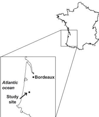
Atlantic ocean

Bordeaux

Study site

Figure 1.Location of the study area in south-western France.

2. To identify individual saproxylic beetle species whose abundance or distribution is correlated with total species species richness, in order to test “species” indicators. 3. To compare “species” and “environmental” indicators on

the basis of their predictive abilities and cost-effectiveness to monitor.

2. MATERIAL AND METHODS 2.1. Study area and sample design

The Landes de Gascogne forest is located in south-western France and is the largest artificial forest of Europe (1 million ha) (Fig.1). It is an intensively managed plantation of Maritime pine (Pinus pinaster Ait.), a native species in this region. Current silvicultural practices are characterized by pure, even-aged stands that are clear-cut harvested at ca 40–50 years, mechanical soil preparation and fertilising, fre-quent thinning, pruning and mechanical removal of the understorey vegetation.

A total of 40 Maritime pine stands were sampled within an area of 64 km2 _{(8 × 8 km) along a systematic grid with sampled stands} arranged in staggered rows. Sampled stands were separated by 2 km along grid lines and by 1.4 km with regards to the diagonal of the staggered row design. In our study the area of stands averaged 17 ha (± 9 ha) and stand age ranged from 5 to 61 years.

2.2. Sampling of woody debris

Dead wood with a diameter of at least 1cm was measured dur-ing autumn 2005. Woody debris was quantified usdur-ing the Line Inter-sect Sampling (LIS) method (De Vries,1973; Marshall et al.,2000).

Downed woody debris > 5 cm Ø was sampled on four 25-m long transects, whereas smaller pieces were assessed on four 5-m long sub-transects per stand. Data from all sub-transects were pooled per stand for statistical analysis. Stumps were assessed using 5 lines of 20 m along tree rows (ca 360 m2_{) or in a circular sub-plot of ca. 710 m}2 _{(15 m} radius) if tree rows were not apparent (old stands). We measured the top diameter of stumps. The height and diameter at breast height of all snags were measured in two circular sub-plots in each stand. The first sub-plot was based on the French National Forest Inventory pro-tocol. It had a variable radius depending on the mean diameter of trees: 6 m (giving a 113 m2 _{area) for trees with diameter less than} 17.5 cm, 9 m (giving a 254 m2_{area) for trees with diameter between} 18 and 27.5 cm and 15 m (giving a 706 m2 _{area) for trees with} di-ameter greater than 28 cm. The second sub-plot consisted of a fixed number of 20 living trees encountered in a spiral-walk. The stage of decomposition of any type of deadwood was qualified according to three classes: (I) fresh, (II) initial decay, (III) advanced decay. We also recorded the species identity of each piece of deadwood. Further details on deadwood sampling and volume computations are provided in Brin et al. (2008).

2.3. Beetle sampling

Beetles were sampled using a PolytrapTM _{window trap (EIP,} France). Each trap consisted of two transparent plastic panes (40 × 60 cm) placed crosswise, with a funnel and a container below the panes. The containers were filled with salt water and some detergent to ensure insect preservation. A total of 80 traps were used, two traps placed ∼ 30 m apart in each sampled stand. The trapping period was from the 10th May to the 30th August 2005. Traps were assessed four times during that period (every 3 to 4 weeks). We identified all indi-viduals of Coleoptera families known to include saproxylic species to the level of species, except for the Corylophidae (due to taxonomi-cal difficulties). Saproxylic beetle families and species were classified according to the life history traits database (FRISBEE) developed by Bouget et al. (2008). As dead wood was mainly derived from Mar-itime pine (99%, unpublished data) we excluded species unable to develop on dead pine wood from further analysis (16% of saproxylic species).

2.4. Data analysis

Beetle abundance at the two traps at each location was pooled to-gether for further analyses. The number of species caught per plot was used as a measure of species diversity. We chose not to standard-ize species richness according to the sample sstandard-ize (by using rarefaction techniques) as samples were collected using a standardised trapping effort. Because of this we consider that differences in the number of individuals caught between sample plots reflected real differences in the abundance of flying beetles.

First the volume of deadwood was calculated for each combina-tion of wood type (downed, stumps, snags), decay stage (I, II, III) and diameter classes (1–2.5 cm, 2.6–5 cm, 5.1–10 cm, 10.1–15 cm, 15.1– 20 cm, > 20 cm), thus providing 54 independent volume descriptors (Tab.I).

An index of deadwood diversity (Dtot1) was calculated as the num-ber of observed combinations formed by the three types (downed, stumps, snags), the three decay stages (I, II, III) and the six diame-ter classes from 1 cm (1–2.5 cm, 2.6–5 cm, 5.1–10 cm, 10.1–15 cm,

(5)

Table I.Deadwood variables used for prediction of the species richness of saproxylic beetles. We used 6 diameter classes and 3 decomposition stages (see Sect. 2 for further details) (DWD: Downed Woody Debris).

Variable Explanation Theoritical range Observed range

Volume descriptors

Vddw_ij Volume of DWD of diameter class “i” and decomposition stage “j” (m3_/ha) _– _0–16.2

Vstp_ij Volume of stumps of diameter class “i” and decomposition stage “j” (m3_/ha) _– _0–6.85

Vsng_ij Volume of snags of diameter class “i” and decomposition stage “j” (m3_/ha) _– _0–17.25 Diversity descriptors

Dtot1 Diversity of all deadwood pieces with a minimum diameter of 1 cm 0–54 2–25

Dddw1 Diversity of downed deadwood pieces with a minimum diameter of 1 cm 0–18 0–13

Dstp1 Diversity of stumps with a minimum diameter of 1 cm 0–18 0–10

Dsng1 Diversity of snags with a minimum diameter of 1 cm 0–18 0–2

15.1–20 cm, > 20 cm), as suggested by Siitonen et al. (2000). Thus Dtot1 values ranged from 0 to 54, and a Dtot1of 54 occurs when at least one piece of deadwood was observed in each of the 54 cate-gories. We computed 3 similar diversity indices for the diversity of downed woody debris, snags and stumps, Dddw1, Dsng1and Dstp1 re-spectively. The values of these three indices ranged from 0 to 18. We calculated the same four indices for diameter classes above 10, 15 and 20 cm, respectively. In total we produced sixteen deadwood diversity descriptors (Tab.I).

Partial Least Square (PLS) regressions were used to relate saprox-ylic beetle richness to predictor variables such as dead wood descrip-tors (Tab.I), abundance or the presence/absence of a single species. PLS regressionscompute latent variables similar to principal compo-nents, but in a way that ensure a good representation of predictor vari-ables and a high correlation with the response variable (Tenenhaus, 1998). This method is a suitable substitute for multiple linear regres-sions in applications that deal with numerous and correlated predictor variables (Tenenhaus,1998). Another advantage of PLS regressions is that they provide a measure of the variable importance in the pro-jection (VIP). Predictors with a VIP-value > 1 are considered to be important at explaining the variation in response variables (Tenen-haus,1998). The most parsimonious model can then be computed by using only these high VIP variables. To assess how many compo-nents are optimal for the model, we plot the root mean squared error of prediction (RMSEP) against the number of components to identify the number of components corresponding to the first local minimum

of the RMSEP (Mevik and Wehrens,2007). The PLS-regression is increasingly used in ecological studies both for dealing with multi-collinearity and identifying important variables (Ekblad et al.,2005; Johansson and Nilsson,2002; Sarthou et al.,2005; Schmidtlein and Sassin,2004).

The search for predictive models in the “environmental” indicator approach was conducted in several steps. First we considered differ-ent subsets of all possible deadwood volume and diversity variables for four minimum diameter thresholds (i.e. 1, 10, 15 and 20 cm). For each subset an initial PLS-regression was computed to give a “com-plete” model and to identify the most relevant predictors (VIP > 1). Those variables were then used to build two parsimonious models for each of the four diameter thresholds. The first one was constituted by all relevant predictors, and the second one, called “diversity model”, only used the diversity variables. As the “diversity model” based on the 15 cm diameter threshold appeared to be the most promising, we went further into the simplification by progressively excluding types (stumps, downed woody debris or snags) or decomposition stages in the set of diversity variables.

We also performed four simple linear regressions with the four most relevant single variables (i.e. volume or diversity of deadwood larger than 1 cm in diameter and volume or diversity of deadwood larger than 15 cm in diameter).

The root mean squared error of prediction (RMSEP) and the co-efficient of determination (R2_{) were used as performance criteria to} compare models. We aimed to minimize the RMSEP and maximize

(6)

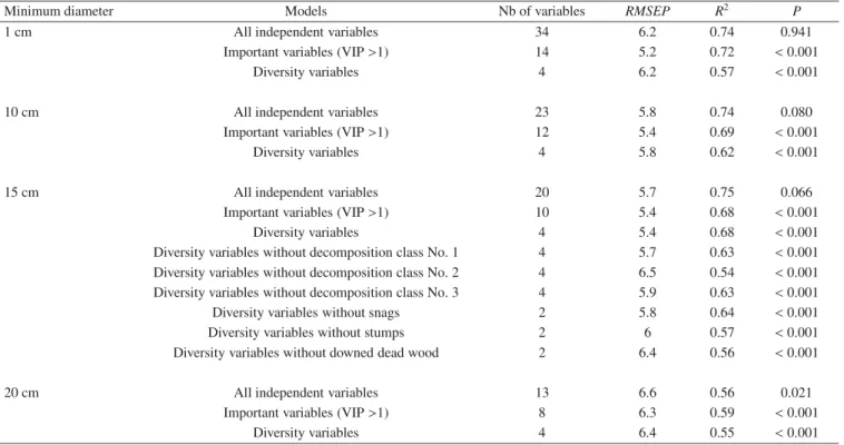
Table II.Results of PLS regressions with deadwood volume and diversity variables as predictors of the species richness of saproxylic beetles (RMSEP: root mean squared error of prediction).

Minimum diameter Models Nb of variables RMSEP R2 _P

1 cm All independent variables 34 6.2 0.74 0.941

Important variables (VIP >1) 14 5.2 0.72 <0.001

Diversity variables 4 6.2 0.57 <0.001

Diversity variables without decomposition class No. 1 4 5.7 0.63 <0.001 Diversity variables without decomposition class No. 2 4 6.5 0.54 <0.001 Diversity variables without decomposition class No. 3 4 5.9 0.63 <0.001 Diversity variables without snags 2 5.8 0.64 <0.001 Diversity variables without stumps 2 6 0.57 <0.001 Diversity variables without downed dead wood 2 6.4 0.56 <0.001

the R2_{, however our dataset was not large enough to allow an} estima-tion of the RMSEP with an independent test set. We therefore used the leave-one-out cross-validation method which is a widely used inter-nal estimation method recommended for determining RMSEP (Mevik and Cederkvist,2004).

For the “species” indicator approach, analyses were conducted on abundance and occurrence (i.e. presence / absence) data. First, we performed a PLS-regression to relate saproxylic species richness to the abundance (or occurrence) of the 93 species that occurred in at least 3 stands (Appendix, available online only at afs-journal.org). The complete model with the 93 independent variables was used to select variables with VIP-value equal or greater than 1. Then, we computed several parsimonious models with groups of a decreasing number of explanatory variables; groups were separated according to dramatic decreases visually noticeable in the histogram of VIP-values.

All analyses were performed with R software (R Development Core Team, 2008) using the pls package (Wehrens and Mevik,2007).

3. RESULTS

3.1. Beetle sample overview

A total of 12 669 individual beetles were caught. Of these, 7 244 individuals were saproxylic beetles belonging to 46 fam-ilies and 240 species. Half of the species were represented by one or two individuals and 201 were known to complete their life-cycle on dead wood of pine. The average number of species per plot was 32.5 (CV = 2 6.6%) and ranged from 19 to 63.

3.2. Relationships between deadwood attributes and richness of saproxylic beetle species

Among the 18 PLS models computed, the one constructed with all deadwood descriptors for ‘wood above 15 cm in di-ameter’ explained the largest proportion of the variance in saproxylic beetle species richness (R2 ₌_{0.75) (Tab.} _II_{). We}

therefore focused on this set of independent variables to look for the most parsimonious models. Two models were of inter-est: one with the 10 variables that showed a VIP value higher than 1 and the second, with only the four "diversity" variables (Tab.II). The same value of RMSEP (5.4) was observed for these two models. Both of them explained an important frac-tion of the variability in species richness with an R2of 0.68. Further reduction in the number of variables entered in the model resulted in higher RMSEP and lower R2_.

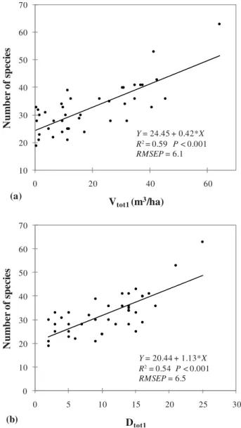
The linear regression models with a single predictor vari-able (Figs.3and4), based on the “diversity index of all pieces of deadwood above 15 cm” in diameter had the lowest RMSEP (5.8) but the best R2_{(0.63) (Fig.}₄_b).

3.3. Relationships between single species abundance or occurrence and species richness of saproxylic beetles

The complete model with 93 single species abundance vari-ables allowed to identify 26 varivari-ables with VIP higher than 1. The model built with these 26 species had good predictive

(7)

DWD (Ø ≥ 5 cm) DWD (1 ≥ Ø < 5 cm) Window traps Snags :

2 sub-plots: one with various radii according to fixed tree diameter and one based on a “spiral-walk” Stumps

Figure 2.Sampling design of deadwood at the stand level (DWD: downed woody debris) and position of the two window traps.

abilities (RMSEP = 4.6, R2₌_{0.82, Tab.}_III_{). A model}

includ-ing the abundance of 6 different species (Tab.III) reached a slightly better explanatory level than those obtained with “en-vironmental” variables (i.e. R2 ₌ _{0.71) for similar RMSEP}

(ca 5.3).

The initial model with 93 species occurrence variables al-lowed to identify 31 variables with VIP higher than 1. The model built with these 31 species had good predicting perfor-mances (RMSEP = 4.3, R2₌_{0.82, Tab.}_IV_{). A model including}

the occurrence of only 7 species (Tab.IV) reached an explana-tory level similar to those obtained with “environmental vari-ables” indicators (i.e. R2₌_{0.67) for similar RMSEP (ca 5.5).}

3.4. Sampling cost

The time required for sampling deadwood in Maritime pine plantations ranged from 20 to 135 min per sampling unit and averaged 52 min for two people involved, giving ca 100 min for one person. It took almost 200 min for one person to as-sess the two window traps in each sampled stand and an addi-tional time of ca. 200 min was needed to sort out and identify saproxylic beetle species. All in all the time spent to quantify the abundance, and estimate the diversity, of saproxylic beetle species captured in each stand was ca 400 min for one person.

4. DISCUSSION 4.1. “Species” indicators

Single species variables (abundance or occurrence) may be of interest to provide an indicator of saproxylic beetle species richness as only 6 to 7 species are required to match the pre-dictive ability of analyses based on environmental variables (Tabs.II,IIIandIV). Some of these species are easy to rec-ognize (e.g. large species such as Prionus coriarius, Hylobius

abietis, Arhopalus rusticus, Spondylis buprestoides), however most can only be identified by a trained entomologist (e.g.

Hylis olexai, Crypturgus cinereus, Anisotoma humeralis). This technical difficulty is a critical drawback of a “species” in-dicator approach. Despite these criticisms the two saprox-ylic beetle species that have been proposed as indicators of species richness in oak forests (Osmoderma eremita and

Cer-ambyx cerdo) are easy to catch and identify (Buse et al.,2008; Ranius,2002). Furthermore the saproxylic beetles suggested by Nilsson et al. (2001) as potential indicators of biodiversity in northern European forests are also species that were easy to identify.

Irrespective of the ease in identification, the time spent trap-ping, identifying and counting individual species of saprox-ylic beetle was four times higher than the time spent sampling deadwood at the stand level. Even if one just wants to focus

(8)

0 10 20 30 40 50 60 70 0 5 10 15 20 25 30 N u mb er o f s p ec ies Dtot1 10 20 30 40 50 60 70 0 20 40 60 N u mb er o f s p ec ies Vtot1 (m3/ha) Y = 24.45 + 0.42*X R2 _{= 0.59 P < 0.001} RMSEP = 6.1 Y = 20.44 + 1.13*X R2_{= 0.54 P < 0.001} RMSEP = 6.5 (a) (b)

Figure 3.Simple linear regressions of saproxylic beetle species rich-ness against the volume (a) and the diversity (b) of deadwood (diam-eter above 1 cm) (RMSEP: root mean squared error of prediction).

on some particular single species in the samples, all individ-ual specimens will have to be sorted out to find the smallest species such as Crypturgus cinereus (2 mm length) or

Aniso-toma humeralis(4 to 5 mm length). Decreasing the number of individual species in predictive models would therefore not result in a proportional time reduction.

4.2. “Environmental” indicators

In the sampled pine plantations, deadwood attributes at the stand-scale were adequate predictors of the saproxylic bee-tle richness and in some cases explained 75% of the vari-ance (Tab.II). There are contrasting results on the relevance of physical variables as predictors of saproxylic species rich-ness. Positive correlations between the volume of deadwood and saproxylic beetle richness at the plot level have frequently

10 20 30 40 50 60 70 0 2 4 6 8 10 12 N u m b er of s p eci es Dtot15 10 20 30 40 50 60 70 80 0 10 20 30 40 50 N u m b er o f s p ec ies Vtot15 (m3/ha) Y = 27.99 + 0.76*X R2_{= 0.57 P < 0.001} RMSEP = 6.1 Y = 23.83 + 2.49*X R2_{= 0.63 P < 0.001} RMSEP = 5.8 (a) (b)

Figure 4.Simple linear regressions of saproxylic beetle species rich-ness against the volume (a) and the diversity (b) of deadwood (diam-eter above 15 cm) (RMSEP: root mean squared error of prediction).

been observed (Grove, 2002, Martikainen et al., McGeoch et al.,2007; 2000; Similä et al.,2003; Sippola et al.,2002); however several authors found no relationships between the local amount of deadwood and the richness of saproxylic bee-tle assemblages (Franc et al.,2007; Økland, et al.,1996; Si-itonen,1994; Similä, et al., 2006;). In our study a portion of the variation in species richness was unexplained by our pre-dictive models. This is illustrated by the intercept value of the linear regressions (Figs.3a and 4a) where a minimum of 20 to 28 saproxylic beetle species was observed irrespective to the local abundance of deadwood. Several reasons may account for these discrepancies. In the cited studies, the ‘local scale’ refers to a broad range of sampled surfaces, from 0.01 ha to 2 ha. Interestingly, all positive and significant effects predic-tions of saproxylic beetle richness based on the local amount of deadwood were observed at a scales between 0.5 ha and

(9)

Table III.Results of PLS regressions with species abundance as predictors of the species richness of saproxylic beetles (RMSEP: root mean squared error of prediction). The number of independent variables (predictors) entered in the model is indicated in brackets.

Species VIP Model 1 (p = 26) Model 2 (p = 23) Model 3 (p = 14) Model 4 (p = 11) Model 5 (p = 6)

Hylastes attenuatus 2.36 × × × × x Hylis olexai 2.15 × × × × x Prionus coriarius 2.13 × × × × x Dacnesp. 2.11 × × × × _x Crypturgus cinereus 2.09 × × × × x Hylobius abietis 2.08 × × × × x Anisotoma humeralis 1.96 × × × × Wanachia triguttata 1.96 × × × × Arhopalus rusticus 1.92 × × × × Rhagium inquisitor 1.89 × × × × Stenagostus rhombeus 1.88 × × × × Brachytemnus porcatus 1.77 × × × Aulonothroscus brevicollis 1.66 × × × Thanasimus formicarius 1.66 × × × Mesocoelopus niger 1.51 × × Enicmus rugosus 1.50 × × Hylurgus ligniperda 1.44 × × Cetonia aurata 1.37 × × Hylastes angustatus 1.36 × × Magdalis memnonia 1.28 × × Diaperis boleti 1.27 × × Ptinus dubius 1.27 × × Anaspis maculata 1.25 × × Xyleborus saxesenii 1.06 × Spondylis buprestoides 1.05 × Berginus tamarisci 1.04 × RMSEP 4.6 4.7 5.9 5.6 5.3 R2 _0.82 _0.79 _0.71 _0.73 _0.71 P 0.061 0.026 0.001 <0.001 <0.001

1 ha (Grove,2002; Martikainen et al.,2000; Sippola et al.,

2002). In contrast the effect was weak to non-existent when sampling at smaller (i.e. 0.01 ha and 0.16 ha) or larger scales (i.e. 2 ha) (Franc et al.,2007; Økland et al.1996; Similä et al.,

2006; Siitonen,1994). This sampling scale effect may reflect differences in the dispersal capabilities of saproxylic beetles; whereby traps can catch long distance flying beetles that did not originate from the sampled stand. The predominance of highly mobile species may decrease the correlation between local deadwood measurements and saproxylic beetles diversity (Jonsson et al.,2005; Nilsson and Baranowski,1997). More-over, in Maritime pine forests it has been shown that wider landscape variables were as important as stand level attributes when assessing local species assemblages of birds, carabids, spiders (Barbaro et al.,2005) and butterflies (Van Halder et al.,

2008).

Deadwood sampling methods may be inappropriate In some circumstances, for example if the sample area is too small as the range in deadwood volume or diversity may be too narrow preventing the identification of significant corre-lations with beetle species richness (Similä et al., 2006). In addition some physical elements are often overlooked, such

as dead branches in the tree crown, polypores or fallen cones that also provide habitat for some saproxylic beetles (Win-ter and Möller,2008). We therefore suggest combining local abundance of several deadwood types to variables measured at broader-scale, such as landscape heterogeneity or fragmenta-tion, to develop betters indicators of saproxylic beetle diver-sity.

One of the main advantages of the “environmental vari-ables” approach is that it saves time in data collection. Fur-thermore, the best and most parsimonious models that we ob-tained were constructed by entering variables that character-ize the volume or diversity of pieces of deadwood larger than 15 cm in diameter. This finding may allow further reductions in the time spent quantifying deadwood as only large pieces would have to be measured.

The relationship between total volume or diversity of dead wood and beetle species richness appeared to be linear (Figs.3

and4). However the number of species cannot increase indefi-nitely as there are limits to the diversity of deadwood. Asymp-totic models such as those proposed by Martikainen et al. (2000) or Norden and Appelqvist (2001) are more ecologically sound, and are analogous to species – area models (MacArthur

(10)

Table IV.Results of PLS regressions with species occurrence (presence/absence) as predictors of the species richness of saproxylic beetles (RMSEP: root mean squared error of prediction). The number of independent variables (predictors) entered in the model is indicated in brackets.

Species VIP Model 1 (p = 31) Model 2 (p = 18) Model 3 (p = 7) Model 4 (p = 5)

Prionus corarius 2.55 × × × x Hylobius abietis 2.35 × × × x Arhopalus rusticus 2.28 × × × x Mycetophagus quadripustulatus 2.18 × × × _x Spondylis buprestoides 2.16 × × × x Anisotoma humeralis 1.84 × × × Hylis olexai 1.81 × × × Dacnesp. 1.65 × × Xyleborus saxesenii 1.65 × × Stenagostus rhombeus 1.64 × × Wanachia triguttata 1.63 × × Hylastes attenuatus 1.57 × × Mesocoelopus niger 1.54 × × Thanasimus formicarius 1.51 × × Cetonia aurata 1.50 × × Crypturgus cinereus 1.47 × × Hylastes angustatus 1.45 × × Stagetus pilula 1.42 × × Dasytes virens 1.29 × Dryophthorus corticalis 1.26 × Anidorus nigrinus 1.19 × Rhagium inquisitor 1.17 × Corymbia rubra 1.15 × Hemicrepidius hirtus 1.15 × Ampedus nigerrimus 1.13 × Hylurgus ligniperda 1.12 × Diaperis boleti 1.11 × Anastrangalia sanguinolenta 1.09 × Magdalis memnonia 1.04 × Aulonothroscus brevicollis 1.03 × Parabaptistes filicornis 1.00 × RMSEP 4.3 4.4 5.5 6.0 R2 0.82 0.8 0.67 0.59 P 0.433 <0.001 <0.001 <0.001

and Wilson,1967). Our linear model may then only account for the initial portion of this asymptotic relationship. To test this hypothesis, investigations would have to be undertaken in stands with greater amounts and diversity of dead wood.

An important outcome of this study is that deadwood diver-sity variables consistently provided similar, or even better, pre-dictive models than volume variables. This is consistent with previous findings about the importance of deadwood qual-ity for saproxylic assemblages (McGeoch et al.,2007; Similä et al.,2003). Diversity variables are probably more informa-tive than abundance variables (i.e. volume per ha) as they may reflect the diversity of available habitats. Saproxylic species communities depend on a wide spectrum of different habitat requirements and the ability of saproxylic species to exploit deadwood as breeding substrate is often restricted to a certain size, type or stage of decay (Jonsell et al.,1998; Schuck et al.,

2004; Siitonen,2001; Stokland et al.,2004). The other inter-est of using diversity variables is that it can reduce the time spent sampling deadwood as presence/absence data from each sub-category of dead wood is sufficient.

4.3. Implications for forestry and biodiversity monitoring

Stand-level indicators are useful because they correspond to an operational scale relevant to forest managers (Failing and Gregory,2003). An interesting feature of structure-based in-dicators such as deadwood volume is that they can be related to silvicultural operations. A model for predicting the volume of downed deadwood and stumps in pine Maritime plantation was developed by combining inputs from thinning operations

(11)

and loss with time (Brin et al., 2008). Now that significant correlations between the volume of deadwood and saproxylic beetle species richness have been found, deadwood accumu-lation can be used to model the effects of alternative forestry practices on saproxylic beetles diversity. This provides a suit-able sustainsuit-able forest management indicator, to evaluate new management options (Noss, 1990). For example, the model could be used to test the effect of shortening the forestry cycle, which would result in lower deadwood volumes and diversity from reduced thinning operations and interruption of the decay process.

It is important to acknowledge that one should not deduce from our datasets and analyses what are the most important deadwood variables for the preservation of saproxylic beetle species richness. As emphasized by Mac Nally (2000), predic-tive models should not be considered as explanatory models. PLS regressions are not appropriate to assess variables that are not important (Vancolen,2004). In our dataset, some vari-ables were excluded from parsimonious models due to lack of variance. Again further investigations are needed to sample deadwood and saproxylic beetles across a wider gradient of forestry conditions, for example in more ancient or less inten-sively managed Maritime pine stands, in order to better iden-tify significant explanatory variables.

Acknowledgements: We are grateful to people involved in the iden-tification of several beetle families: Pascal Leblanc, Pierre Berger, Christophe Bouget, Thierry Noblecourt, Éric de Laclos, Laurent Schott, Gianfranco Liberti, Marc Tronquet, Patrick Dauphin, Jean-Philippe Tamisier and Bernard Moncoutier. We are also grateful to Lionel Valladares for his help with the fieldwork and Meghan An-derson and Steve Pawson who read and commented an early version of this manuscript. Support for this project came from the project “Sustainable Forest management: a network of pilot zones for oper-ational implementation (FORSEE)” financed by the European Union (FEDER) and from the project RESINE financed by the Groupement

d’Intérêt PublicECOFOR.

REFERENCES

Bader P., Jansson S., and Jonsson B.G., 1995. Wood-inhabiting fungi and substratum decline in selectively logged boreal spruce forests. Biol. Conserv. 72: 355–362.

Barbaro L., Pontcharraud L., Vétillard F., Guyon D., and Jactel H., 2005. Comparative responses of birds, carabid, and spider assemblages to stand and landscape diversity in Maritime pine plantation forests. Ecoscience 12: 110–121.

Bouget C., Brustel H., and Zagatti P., 2008. The French information sys-tem on saproxylic beetle ecology (FRISBEE): an ecological and tax-onomical database to help with the assessment of forest conservation status. Rev. Ecol. (Terre Vie) Suppl. 10: 33–36.

Brin A., Meredieu C., Piou D., Brustel H., and Jactel H., 2008. Changes in quantitative patterns of dead wood in Maritime pine plantations over time. For. Ecol. Manage. 256: 913–921.

Buse J., Ranius T., and Assmann T., 2008. An endangered longhorn bee-tle associated with old oaks and its possible role as an ecosystem engineer. Conserv. Biol. 22: 329–337.

Bütler R., Angelstam P., Ekelund P., and Schlaeffer R., 2004. Dead wood threshold values for the three-toed woodpecker presence in boreal and sub-Alpine forest. Biol. Conserv. 119: 305–318.

De Vries P.G., 1973. A general theory on line intersect sam-pling with application to logging residue inventory. Mededelingen Landbouwhogeschool, 73–11, Wageningen,The Netherlands. Duelli P. and Obrist M.K., 2003. Biodiversity indicators: the choice of

values and measures. Agric. Ecosyst. Environ. 98: 87–98.

EEA, 2007. Halting the loss of biodiversity by 2010: proposal for a first set of indicators to monitor progress in Europe. Rep. No. 11/2007, Copenhagen, 186 p.

Ekblad A., Boström B., Holm A., and Comstedt D., 2005. Forest soil res-piration rate and d13_{C is regulated by recent above ground weather}

conditions Oecologia 143: 136–142.

Elton C.S., 1966. Dying and dead wood. In: Elton C.S. (Ed.), The Pattern of Animal Communities, Chapman and Hall, New York, pp. 279– 305.

Failing L. and Gregory R., 2003. Ten common mistakes in designing bio-diversity indicators for forest policy. J. Environ. Manag.68: 121–132. Franc N., Gotmark F., Økland B., Norden B., and Paltto H., 2007. Factors and scales potentially important for saproxylic beetles in temperate mixed oak forest. Biol. Conserv. 135: 86–98.

Grove S.J., 2002. Tree basal area and dead wood as surrogate indicators of saproxylic insect fauna integrity: a case study from the Australian lowland tropics. Ecol. Indic. 1: 171–188.

Hansson L., 2001. Indicators of biodiversity: recent approaches and some general suggestions. Ecol. Bull. 50: 223–229.

Humphrey J.W., Davey S., Peace A.J., Ferris R., and Harding K., 2002. Lichens and bryophyte communities of planted and semi-natural forests in Britain: the influence of site type, stand structure and dead-wood. Biol. Conserv. 107: 165–180.

Jacobs J.M., Spence J.R., and Langor D.W., 2007. Influence of boreal for-est succession and dead wood qualities on saproxylic beetles. Agric. For. Entomol. 9: 3–16.

Johansson M.E. and Nilsson C., 2002. Responses of riparian plants to flooding in free-flowing and regulated boreal rivers: an experimental study J. Appl. Ecol. 39: 971–986.

Jonsell M., Weslien J., and Ehnstrom B., 1998. Substrate requirements of red-listed saproxylic invertebrates in Sweden. Biodivers. Conserv. 7: 749–764.

Jonsson B.G., Kruys N., and Ranius T., 2005. Ecology of species living on dead wood – Lessons for dead wood management. Silva Fenn. 39: 289–309.

Larsson T.-B., Angelstam P., Balent G., Barbati A., Bijlsma R.-J., Boncina A., Bradshaw R., Bücking W., Ciancio O., Corona P., Diaci J., Dias S., Ellenberg H., Fernandes F.M., Fernandez-Gonzalez F., Ferris R., Frank G., Møller P.F., Giller P.S., Gustafsson L., Halbritter K., Hall S., Hansson L., Innes J., Jactel H., Keannel Dobbertin M., Klein M., Marchetti M., Mohren F., Niemelä P., O’Halloran J., Rametsteiner E., Rego F., Scheidegger C., Scotti R., Sjöberg K., Spanos I., Spanos K., Standovár T., Svensson L., Åge Tømmerå B., Trakolis D., Uuttera J., VanDenMeersschaut D., Vandekerkhove K., Walsh P.M., and Watt A.D., 2001. Biodiversity evaluation tools for European forests. Ecol. Bull. 50: 127–139.

Lindenmayer D.B., Margules C.R., and Botkin D.B., 2000. Indicators of biodiversity for ecologically sustainable forest management. Conserv. Biol. 14: 941–950.

MacArthur R.H. and Wilson E.O., 1967. The theory of island biogeogra-phy. Princeton University Press, 203 p.

Mac Nally R., 2000. Regression and model-building in conservation biology, biogeography and ecology: The distinction between and reconciliation of “predictive” and “explanatory” models. Biodivers. Conserv. 9: 655–671.

Mac Nally R., Parkinson A., Horrocks G., Conole L., and Tzaros C., 2001. Relationships between terrestrial vertebrate diversity, abun-dance and availability of coarse woody debris on south-eastern Australian floodplains. Biol. Conserv. 99: 191–205.

(12)

Marshall P.L., Davis G., and LeMay V.M., 2000. Using line intersect sam-pling for coarse woody debris. Rep. TR-003, Forest Service, British Columbia, Vancouver Forest Region, 34 p.

Martikainen P., Siitonen J., Punttila P., Kaila L., and Rauh J., 2000. Species richness of Coleoptera in mature managed and old-growth boreal forests in southern Finland. Biol. Conserv. 94: 199–209. McGeoch M.A., Schroeder M., Ekbom B., and Larsson S., 2007.

Saproxylic beetle diversity in a managed boreal forest: importance of stand characteristics and forestry conservation measures. Divers. Distrib. 13: 418–429.

MCPFE, 2003. Improved Pan-European indicators for sustainable forest management. Rep. MCPFE Liaison Unit Vienna, Vienna, 6 p. Mevik B.H. and Cederkvist H.R., 2004. Mean squared error of

predic-tion (MSEP) estimates for principal component regression (PCR) and partial least squares regression (PLSR). J. Chemometr. 18: 422–429. Mevik B.H. and Wehrens R., 2007. The pls package: principal component

and partial least squares regression in R. J. Stat. Soft. 18: 1–24. Nilsson S.G. and Baranowski R., 1997. Habitat predictability and the

oc-curence of wood beetles in old-growth beech forests. Ecography 20: 491–498.

Nilsson S.G., Hedin J., and Niklasson M., 2001. Biodiversity and its assessment in boreal and nemoral forests. Scand. J. Forest. Res. 3: 10–26.

Norden B. and Appelqvist T., 2001. Conceptual problems of ecological continuity and its bioindicators. Biodivers. Conserv. 10: 779–791. Noss R., 1990. Indicators for monitoring biodiversity: a hierarchical

ap-proach. Conserv. Biol. 4: 355–364.

Noss R., 1999. Assessing and monitoring forest biodiversity: a suggested framework and indicators. For. Ecol. Manage. 115: 135–146. Økland B., Bakke A., Hagvar S., and Kvamme T., 1996. What factors

in-fluence the diversity of saproxylic beetles? A multiscaled study from a spruce forest in southern Norway. Biodivers. Conserv. 5: 75–100. Pentillä R., Siitonen J., and Kuusinen M., 2004. Polypore diversity in

managed and old-growth boreal Picea abies forests in southern Finland. Biol. Conserv. 117: 271–283.

R Development Core Team, 2008. R: A language and environment for sta-tistical computing. R Foundation for Stasta-tistical Computing, Vienna, Austria. ISBN 3-900051-07-0, URLhttp://www.R-project.org. Ranius T., 2002. Osmoderma eremita as an indicator of species richness

of beetles in tree hollows. Biodivers. Conserv. 11: 931–941. Ranius T. and Jonsson M., 2007. Theoretical expectations for

thresh-olds in the relationship between number of wood-living species and amount of coarse woody debris: A study case in spruce forests. J. Nat. Conserv. 15: 120–130.

Sætersdal M., Gjerde I., and Blom H.H., 2005. Indicator species and the problem of spatial inconsistency in nestedness patterns. Biol. Conserv. 122: 305–316.

Sarthou J.-P., Ouin A., Arrignon F., Barreau G., and Bouyjou B., 2005. Landscape parameters explain the distribution and abundance of

Episyrphus balteatus(Diptera : Syrphidae). Eur. J. Entomol. 102: 539–545.

Schlaepfer R. and Bütler R., 2004. Critères et indicateurs de la gestion des ressources forestières : prise en compte de la complexité et de l’approche écosystémique. Rev. For. Fr. LVI: 431–444.

Schmidtlein S. and Sassin J., 2004. Mapping of continuous floristic gradients in grasslands using hyperspectral imagery. Remote. Sens. Environ. 92: 126–138.

Schuck A., Meyer P., Menke N., Lier M., and Lindner M., 2004. Forest biodiversity indicator: dead wood – a proposed approach to-wards operationalising the MCPFE indicator. In: Marchetti M. (Ed.), Monitoring and indicators of forest biodiversity in Europe – from ideas to operationality, EFI Proceedings, pp. 49–77.

Siitonen J., 1994. Decaying wood and saproxylic Coleoptera in two old spruce forests: a comparison based on two sampling methods. Ann. Zool. Fenn. 31: 89–95.

Siitonen J., 2001. Forest management, coarse woody debris and saprox-ylic organisms : Fennoscandian boreal forests as an example. Ecol. Bull. 49: 11–41.

Siitonen J., Martikainen P., Punttilä P., and Rauh J., 2000. Coarse woody debris and stand characteristics in mature managed and old-growth boreal mesic forests in southern Finland. For. Ecol. Manage. 128: 211–225.

Similä M., Kouki J., and Martikainen P., 2003. Saproxylic beetles in man-aged and seminatural Scots pine forests: quality of dead wood mat-ters. For. Ecol. Manage.174: 365–381.

Similä M., Kouki J., Monkkonen M., Sippola A.L., and Huhta E., 2006. Co-variation and indicators, of species diversity: Can richness of forest-dwelling species be predicted in northern boreal forests? Ecol. Indic. 6: 686–700.

Sippola A.L., Siitonen J., and Punttila P., 2002. Beetle diversity in tim-berline forests: a comparison between old-growth and regeneration areas in Finnish Lapland. Ann. Zool. Fenn. 39: 69–86.

Smith G.F., Gittings T., Wilson M., French L., Oxbrough A., O’Donoghue S., O’Halloran J., Kelly D.L., Mitchell F.J.G., Kelly T., Iremonger S., McKee A.-M., and Giller P., 2008. Identifying practical indica-tors of biodiversity for stand-level management of plantation forests. Biodivers. Conserv. 17: 991–1015.

Stokland J.N., Tomter S.M., and Söderber U., 2004. Development of Dead Wood Indicators for Biodiversity Monitoring: Experiences from Scandinavia. In: Marchetti M. (Ed.), Monitoring and Indicators of forest biodiversity in Europe – from ideas to operationality, EFI Proceedings, 207–226.

Stokland J.N. and Meyke E., 2008. The saproxylic database: an emerging overview of the biological diversity in dead wood. Rev. Ecol. (Terre Vie) Suppl. 10 : 37–48.

Tenenhaus M., 1998. La régression PLS. Théorie et pratique, Editions Technip, Paris, 254 p.

Van Halder I., Barbaro L., Corcket E., and Jactel H., 2008. Importance of semi-natural habitats for the conservation of butterfly communities in landscapes dominated by pine plantations. Biodivers. Conserv. 17: 1149–1169.

Vancolen S., 2004. La régression PLS. Université de Neuchâtel, Suisse, 28 p.

Wehrens R. and Mevik B.H., 2007. The pls package: partial least squares regression (PLSR) and principal component regression (PCR). Winter S. and Möller G.C., 2008. Microhabitats in lowland beech forests

as monitoring tool for nature conservation. For. Ecol. Manage. 255: 1251–1261.